HAL Id: hal-00522647
https://hal.archives-ouvertes.fr/hal-00522647
Submitted on 1 Oct 2010
HAL is a multi-disciplinary open access
archive for the deposit and dissemination of
sci-entific research documents, whether they are
pub-lished or not. The documents may come from
teaching and research institutions in France or
abroad, or from public or private research centers.
L’archive ouverte pluridisciplinaire HAL, est
destinée au dépôt et à la diffusion de documents
scientifiques de niveau recherche, publiés ou non,
émanant des établissements d’enseignement et de
recherche français ou étrangers, des laboratoires
publics ou privés.
Penalized Direct Forcing and Projection Schemes for
Navier-Stokes
Michel Belliard, Clarisse Fournier
To cite this version:
Michel Belliard, Clarisse Fournier. Penalized Direct Forcing and Projection Schemes for
Navier-Stokes. Comptes rendus de l’Académie des sciences. Série I, Mathématique, Elsevier, 2010, 248
(19-20), pp.1133-1136. �hal-00522647�
Penalized Direct Forcing and Projection Schemes for
Navier-Stokes
Michel Belliard
bClarisse Fournier
cCEA, D´epartement d’Etudes des R´eacteurs, DEN/DER/SSTH b
CEA, DEN, DER/SSTH/LDAL - Cadarache, F-13108 St Paul-lez-Durance, France c
CEA, DEN, DER/SSTH/LDAL, F-38054 Grenoble, France Received *****; accepted after revision +++++
Presented by
Abstract
This note presents a new method of direct forcing to deal with obstacles in incompressible flows. It mixes projection
schemes and velocity L2
penalty schemes. The penalized direct forcing term is distributed in the velocity prediction and the correction equations. It leads to a natural treatment in the correction equation of the boundary conditions
in pressure around obstacles. A numerical experiment provided an illustration of the method.To cite this article:
M. Belliard, C. R. Acad. Sci. Paris, Ser. I 340 (2005).
R´esum´e
M´ethode de For¸cage Direct P´enalis´e et Sch´emas de Projection pour Navier-Stokes. Cette note
pr´esente une nouvelle m´ethode de for¸cage directe pour prendre en compte des obstacles dans un ´ecoulement
incompressible. Elle m´elange m´ethodes de projection et de p´enalisation L2 des vitesses. La ventilation du terme
de for¸cage direct p´enalis´e dans les ´equations de pr´ediction et de correction conduit `a un traitement naturel des
conditions aux limites pour la correction de pression aux bords des obstacles. Une exp´erience num´erique est
pr´esent´ee `a titre d’illustration. Pour citer cet article : M. Belliard, C. R. Acad. Sci. Paris, Ser. I 340 (2005).
1. Introduction
The well-known incompressible Navier-Stokes equations allow the description of the behavior of incom-pressible flows (div u = 0 with u the fluid velocity). Mass and momentum balance equations in the fluid
domain Ωf read as (with Dirichlet boundary conditions -BC -, u = uD on ∂Ωf):
∂tu+ u ⊗ ∇u + ρ−1∇p − div(ν∇u) = f in Ωf
div u = 0 in Ωf
(1) with p the pressure, ρ the (constant) density, ν the cinematic viscosity and f the volume force.
The projection method (or fractional step method) for an incompressible fluid was introduced by Chorin
and Temam in 1968 [2,10]. The incremental projection scheme of Shen [9] reads as follow.1 First, a non
divergence free velocity eu is predicted using the previous time step pressure. For example, a linearized
implicit Euler time discretization2, with un,∗given by an Adam-Bashforth scheme, leads to:
e
u − un
∆t + u
n,∗⊗ ∇eu+ ρ−1∇pn−div(ν∇eu) = fn+1 in Ω
f and eu= uD on ∂Ωf. (2)
Second, with the hypothesis div (ν∇eu) ∼ div (ν∇un+1) and un,∗⊗ ∇eu ∼ un,∗⊗ ∇un+1, a correction
stage is performed to recover the divergence free velocity un+1:
un+1−ue ∆t = −ρ −1∇φn+1 in Ω f and un+1= uD on ∂Ωf div un+1 = 0 in Ωf (3)
with φn+1= pn+1−pnthe pressure correction. Considering the divergence free condition, we are able to
compute φn+1 and so on the divergence free velocity un+1and the new pressure pn+1by:
div ∇φn+1= ρ
∆tdiveu in Ωf and ∇φ
n+1· n= 0 on ∂Ω
f. (4)
2. Direct Forcing
In the context of the Fictitious Domain methods, the Immersed Boundary Method was introduced by
Peskin at the beginning of 1970 [8]. Considering obstacles in a flow, the fluid domain Ωf is extended to
Ω including the obstacle domain Ωs: Ω = Ωf∪Ωs. A body force is added to the momentum equation to
take into account the obstacle. In 1997 Mohd-Yusof introduces the Direct Forcing method [7]:
un+1− un
∆t = Tn,n+1+ Fn,n+1 in Ω (5)
with here Tn,n+1 = fn+1− un,∗⊗ ∇un+1−ρ−1∇pn+1+ div (ν ∇un+1). The forcing term is defined as:
Fn,n+1= χs[
(vn+1
s − un)
∆t − Tn,n+1] (6)
with vsthe imposed fluid velocity around/inside the obstacle and χs : R3→ Rthe discrete characteristic
function or the volume ratio function of the obstacle, see [3].
Remark 1 The imposed velocity vsneeds to be interpolated from the fluid velocity field euand the boundary
condition to improve the accuracy (vs= ¯εu, see Fadlun et al. [3]).e
Remark 2 The direct forcing should be taken into account into the projection equation (4) through the
interpolation matrix ¯ε (div ¯ε∇φ = ∆tρ divue) to get a free divergence velocity respecting the boundary
conditions (consistent scheme, see Ikeno et al. [5]).
1
Projection schemes for dilatable or barotropic fluid can be found in [4,6]. 2
Using the Crank-Nicholson time scheme should be worth, but it isn’t the goal of this Note.
In this new method, the following forcing term is added to the right hand side of Navier-Stokes equa-tions: Fn+1= χs η∆t(v n+1 s − un+1) with 0 < η ≪ 1. (7)
It can be viewed as an implicit forcing term cχs
∆t(vs− u) as well as a velocity L
2penalty term cχs
η (vs−
u) [1]. As for the Direct Forcing, interpolations can be used to determine the imposed velocity vs. In the
following, un+1is the solution of penalized Navier-Stokes. Lets define un+1
η := limη→0un+1. Then, we have
un+1
η ∼ vn+1s . Following Angot et al. [1], un+1η converges toward the N.-S. body fitted solution in L2(Ωs)
norm with order ≤ 3/4 in η. The new feature of our algorithm is that the forcing term (7) is distributed in the prediction and the correction stages of the projection leading to a natural consistent scheme:
e u − un ∆t + u n,∗⊗ ∇eu+ ρ−1∇pn−div ν∇eu= fn+1+ χs η∆t(v n+1 s −u)e in Ω un+1−eu ∆t = −ρ −1∇φn+1+ χs η∆t(eu − u n+1) in Ω (8)
The first equation of (8) leads to the penalized predicted velocity: euη := lim
η→0eu ∼ v
n+1
s in Ωs. Hence
the Dirichlet boundary conditions of (2) are locally enforced on ∂Ωf ∩∂Ωs. The second equation of (8)
suggests:
un+1−ue
∆t = − ˇρ
−1∇φn+1 in Ω with suitable BC on ∂Ω. (9)
This equation is similar to the first one of (3) with ˇρ:= ρ(1 +χs
η) justifying the introduction of the term
∆t in (7). For χs= 0, we have ˇρ= ρ and lim
η→0ρ(η) ≈ O(ηˇ
−1) for χ
s >0. Using div un+1= 0 in Ωf and
div un+1= div v
s in Ωs, instead of the second equation of (3), we get a slightly modification of the first
equation of (4): div η η+ χs ∇φn+1= ρ ∆t(div eu − χsdiv v n+1 s ) in Ω with suitable BC on ∂Ω. (10)
Lets remark that, in case of solid rotations and/or translations, div vs= 0 in Ωs. For χs= 1, we have an
effective diffusion coefficient 1+ηη ≈ O(η) ≪ 1. Then, the homogeneous Neumann boundary conditions
of (4) are locally enforced on ∂Ωf∩∂Ωsin a natural way. Finally, the correction equation (9) allows the
computation of un+1. We have un+1
η ∼ueη∼ vn+1s in Ωs
Remark 3 In Ωs, all the diffusion coefficients may vanish leading to numerical problems solving (10).
Then, adding a pressure L2 penalty term can be a cure, leading to a different formulation of the pressure
correction equation (where φ0 is a prescribed pressure correction):
div O(η)∇φn+1+1 η(φ n+1−φ 0) = ρ ∆t(div eu − div v n+1 s ) in Ωs. (11) 4. Numerical experiments
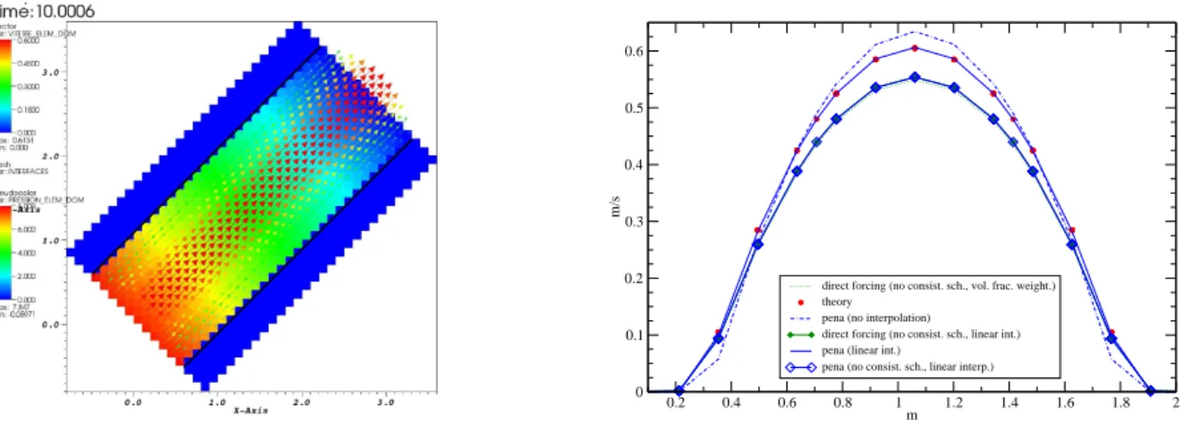
Fig. 1, left, shows a 2D Poiseuille flow in a square channel rotated of 45˚with regard to the Cartesian mesh. Immersed Boundaries define the solid walls (black lines). Imposed near-wall velocities are linearly
0.2 0.4 0.6 0.8 1 1.2 1.4 1.6 1.8 2 m 0 0.1 0.2 0.3 0.4 0.5 0.6 m/s
direct forcing (no consist. sch., vol. frac. weight.) theory
pena (no interpolation)
direct forcing (no consist. sch., linear int.) pena (linear int.)
pena (no consist. sch., linear interp.)
Figure 1. Poiseuille Flow: Direct Forcing and Penalized Direct Forcing. Left: Velocity and pressure fields (linearly interpolated Penalized Direct Forcing). Right: Velocity profiles (no interpolation or linear interpolation, no consistent or consistent scheme).
interpolated from the nearest free fluid velocities and the boundary conditions vn+1
s = ¯εun. Computations
are done using the CEA CFD code Trio U [11]. The value of the penalty coefficient η is 10−12. Velocity
profiles, obtained by the linearly interpolated Penalized Direct Forcing method, compare very well to the theoretical ones, see Fig. 1, right. Without consistent schemes the theoretical velocities are missed
whatever the interpolation is. Moreover, the numerical order of the method remains about 2 in L2norm
when using a second order discretization for the spatial operators. References
[1] Ph. Angot, Ch.-H. Bruneau, P. Fabrie, A penalization method to take into account obstacles in incompressible viscous flows, Numerische Mathematik 81 (1999) 497-520.
[2] A. Chorin, Numerical Solution of the Navier-Stokes Equations, Mathematics of Computation 22 (1968) 745-762. [3] E. A. Fadlun, R. Verzicco, P. Orlandi, J. Mohd-Yusof, Combined Immersed-Boundary Finite-Difference Methods for
Three-Dimensional Complex Flow Simulations, Journal of Computational Physics 161 (2000) 35-60.
[4] Th.Gallou¨et, L. Gastaldo, R. Herbin, J.-C. Latch´e, An unconditionally stable pressure correction scheme for the compressible barotropic Navier-Stokes equations, M2AN 42 (2008) 303-331.
[5] T. Ikeno, T. Kajishima, Finite-difference immersed boundary method consistent with wall conditions for incompressible turbulent flow simulations, Journal of Computational Physics 226 (2007) 1485-1508.
[6] M. Jobelin, B. Piar, Ph. Angot, J.-C. Latch´e, Une m´ethode de p´enalit´e-projection pour les ´ecoulements dilatables, European J. Comput. Mech. 17 (2008) 453 480.
[7] J. Mohd-Yusof, Combined Immersed Boundaries/B-Splines Methods for Simulations of Flows in Complex Geometries, CTR Annual Research Briefs, NASA Ames/Stanford University, 1997.
[8] C. Peskin, Numerical Analysis of blood flow in heart, Journal of Computational Physics 25 (1977) 220-252.
[9] J. Shen, On Error Estimates of some Higher Order Projection and Penalty-Projection Methods for Navier-Stokes Equations, Numerische Mathematik. 62 (1992) 49-73.
[10] R. Temam, Sur l’approximation de la solution des ´equations de Navier-Stokes par la m´ethode des pas fractionnaires, Arch.Rational Mech. Anal. 32 (1969) 135-153.
[11] http://www-trio-u.cea.fr