HR-COSMOS: Kinematics of star-forming galaxies at z $\sim$ 0.9

HAL Id: hal-01582433

https://hal.archives-ouvertes.fr/hal-01582433

Submitted on 16 Jan 2021

HAL is a multi-disciplinary open access

archive for the deposit and dissemination of

sci-entific research documents, whether they are

pub-lished or not. The documents may come from

teaching and research institutions in France or

abroad, or from public or private research centers.

L’archive ouverte pluridisciplinaire HAL, est

destinée au dépôt et à la diffusion de documents

scientifiques de niveau recherche, publiés ou non,

émanant des établissements d’enseignement et de

recherche français ou étrangers, des laboratoires

publics ou privés.

HR-COSMOS: Kinematics of star-forming galaxies at z

∼ 0.9

D. Pelliccia, L. Tresse, B. Epinat, O. Ilbert, N. Scoville, P. Amram, B.C.

Lemaux, G. Zamorani

To cite this version:

D. Pelliccia, L. Tresse, B. Epinat, O. Ilbert, N. Scoville, et al.. HR-COSMOS: Kinematics of

star-forming galaxies at z

_{∼ 0.9. Astron.Astrophys., 2017, 599, pp.A25. �10.1051/0004-6361/201629064�.}

�hal-01582433�

A&A 599, A25 (2017) DOI:10.1051/0004-6361/201629064 c ESO 2017

Astronomy

&

Astrophysics

HR-COSMOS: Kinematics of star-forming galaxies at z

∼

_0.9

?

D. Pelliccia

, L. Tresse

, B. Epinat

, O. Ilbert

, N. Scoville

, P. Amram

, B. C. Lemaux

, and G. Zamorani

1 _{Aix Marseille Université, CNRS, LAM (Laboratoire d’Astrophysique de Marseille) UMR 7326, 13388 Marseille, France}

e-mail: debora.pelliccia@lam.fr

2 _{Univ. Lyon, ENS Lyon, Univ. Lyon 1, CNRS, Centre de Recherche Astrophysique de Lyon UMR5574, 69007 Lyon, France} 3 _{California Institute of Technology, MC 249-17, 1200 East California Boulevard, Pasadena, CA 91125, USA}

4 _{University of California Davis, 1 Shields Avenue, Davis, CA 95616, USA} 5 _{INAF–Osservatorio Astronomico di Bologna, via Ranzani 1, 40127 Bologna, Italy}

Received 6 June 2016/ Accepted 19 September 2016

ABSTRACT

We present the kinematic analysis of a sub-sample of 82 galaxies at 0.75 < z < 1.2 from our new survey HR-COSMOS aimed to obtain the first statistical sample to study the kinematics of star-forming galaxies in the treasury COSMOS field at 0 < z < 1.2. We observed 766 emission line galaxies using the multi-slit spectrograph ESO-VLT/VIMOS in high-resolution mode (R = 2500). To better extract galaxy kinematics, VIMOS spectral slits have been carefully tilted along the major axis orientation of the galaxies, making use of the position angle measurements from the high spatial resolution HST/ACS COSMOS images. We constrained the kinematics of the sub-sample at 0.75 < z < 1.2 by creating high-resolution semi-analytical models. We established the stellar-mass Tully-Fisher relation at z ' 0.9 with high-quality stellar mass measurements derived using the latest COSMOS photometric catalog, which includes the latest data releases of UltraVISTA and Spitzer. In doubling the sample at these redshifts compared with the literature, we estimated the relation without setting its slope, and found it consistent with previous studies in other deep extragalactic fields assuming no significant evolution of the relation with redshift at z. 1. We computed dynamical masses within the radius R2.2and found a median

stellar-to-dynamical mass fraction equal to 0.2 (assuming Chabrier IMF), which implies a contribution of gas and dark matter masses of 80% of the total mass within R2.2, in agreement with recent integral field spectroscopy surveys. We find no dependence of the

stellar-mass Tully-Fisher relation with environment probing up to group scale masses. This study shows that multi-slit galaxy surveys remain a powerful tool to derive kinematics for large numbers of galaxies at both high and low redshift.

Key words. galaxies: evolution – galaxies: kinematics and dynamics – galaxies: high-redshift – galaxies: statistics – surveys

1. Introduction

In the local Universe, we distinguish a clear bimodality dis-tribution of galaxies in two types with red and blue rest-frame colors, commonly referred to as the red sequence and blue cloud, with a lack of galaxies at intermediate colors (Blanton et al. 2003; Baldry et al. 2004). These color classes are strongly correlated with morphology, so that the blue cloud region is mostly populated by rotating star-forming galaxies (usually spiral) and on the red sequence we find generally qui-escent ellipticals, though there is a rare population of red spirals which overlaps the red sequence and may arise from truncated star formation (Masters et al. 2010;Cortese 2012). Star-forming galaxies at high redshift (z > 0.1) exhibit a larger diversity of kinematics than in the local Universe (z  0.1), and higher fractions of such galaxies are not dominated by rotation or have complex kinematic signatures owing to merging processes (Conselice et al. 2003;Hammer et al. 2009;Kassin et al. 2012; Puech et al. 2012).

Kinematics enables us to trace galaxy properties from high to low redshift and to constrain the galaxy formation scenario us-ing, for example, the well established scaling relation for rotat-ing galaxies observed for the first time byTully & Fisher(1977) between the optical luminosity and HI line width. The Tully-Fisher (TF) relation is a key to understand the structure and

? _{Based on observations made with ESO Telescopes at the La Silla}

Paranal Observatory under programme ID 083.A-0935.

evolution of disc galaxies, since it probes the dark matter halos with their luminous baryonic components, and thus constrains the galaxy formation and evolution models (e.g.,Dalcanton et al. 1997;Sommer-Larsen et al. 2003). Later works have shown that the TF relation becomes tighter when defined using microwave to infrared luminosity (Verheijen 1997), and even tighter when luminosity is replaced by the galaxy’s stellar mass (Pizagno et al. 2005) or total baryonic mass (McGaugh 2005).

The stellar mass Tully-Fisher (smTF) relation has been stud-ied in the local Universe (Bell & de Jong 2001; Pizagno et al. 2005;Courteau et al. 2007;Reyes et al. 2011) and it appears to be remarkably tight. However, the relation is not yet well defined at higher redshift. Past studies have investigated possible evolu-tion of the smTF relaevolu-tion with conflicting results.Conselice et al. (2005) was the first to look at the smTF relationship at inter-mediate redshift using the longslit spectroscopy technique with a sample of 101 disc galaxies with near-IR photometry, fin-ding no evidence for an evolution of the relation from z= 0 to z= 1.2.Puech et al.(2008,2010) constrained the smTF relation at z ∼ 0.6 for a small sample of 16 rotating disc galaxies (out of 64 analyzed), part of the IMAGES survey, and they found an evolution of the relation towards lower stellar masses. A slit-based survey with DEIMOS multi-object spectrograph on Keck (Faber et al. 2003) was presented by Miller et al. (2011) who have sampled a larger number of galaxies (N = 129) at 0.2 < z < 1.3, showing no statistically significant evolution of the smTF relation, though an evident evolution of the B-band

TF with a decrease in luminosity of ∆MB = 0.85 ± 0.28 mag

from hzi ' 1.0 to 0.3.

Furthermore, it is unclear whether an evolution with red-shift of the intrinsic scatter around the TF relation exists. Kannappan et al.(2002) have shown how the scatter around the TF relation in the local Universe increases by broaden-ing their spiral sample, for which the relation is computed, to include all morphologies. Since galaxies at higher red-shift show more irregular morphology (Glazebrook et al. 1995; Förster Schreiber et al. 2009), we expect to observe an increase in the scatter with redshift. Puech et al. (2008, 2010) argue that the increase in intrinsic scatter around the TF relation was due to the galaxies with complex kinematics.Kassin et al. (2007), as well, looking at the smTF relationship of 544 galaxies (0.1 < z < 1.2) from the DEEP2 redshift survey (Newman et al. 2013a), have found a large scatter (∼1.5 dex in velocity) domi-nated by the more disturbed morphological classes and the lower stellar masses. Conversely Miller et al. (2011) reported a very small intrinsic scatter around the smTF relation throughout their whole sample at 0.2 < z < 1.3.

The large scatter around the TF relation for broadly selected samples, may also depend on properties external to the galaxies. Environment, for example, is known to have a strong impact on galaxy parameters (Baldry et al. 2006;Bamford et al. 2009; Capak et al. 2007; Sobral et al. 2011; Scoville et al. 2013) and we could expect to see environmental effects also on the TF relation. An alteration in the TF relation in a dense environ-ment, for example, could be due to a temporary increase of the star formation activity or to kinematic asymmetry owing to dynamical interaction of galaxies. Nevertheless, studies on the effects of the environment on the TF relation are still few. Mocz et al.(2012) constrained the TF relation in the u, g, r, i, and z bands and smTF for a local Universe sample of 25 698 late spiral galaxies from the Sloan Digital Sky Survey (SDSS) and investigated any dependence of the relation from the envi-ronment defined using the local number density of galaxies as a proxy to their host region. They found no strong or statisti-cally significant changes in the TF relation slope or intercept. At intermediate redshifts, some works constrained the TF rela-tion for cluster and field galaxies, but the results are highly dis-cordant.Ziegler et al.(2003) compared the B-band TF relation for a small sample of 13 galaxies from three clusters at z= 0.3, z= 0.42 and z = 0.51 and 77 field galaxies at 0 < z < 1 observed with the same set up of the clusters, and they have found no sig-nificant differences. The same result of no environmental effect was presented byNakamura et al.(2006) for a still small sample of 13 cluster galaxies and 20 field galaxies between z= 0.23 and z= 0.58. Conversely,Bamford et al.(2005) with a larger sample of 80 galaxies at 0 < z < 1 (22 in clusters and 58 in the field) have found a systematic offset of ∆MB = 0.7 ± 0.2 mag in the

B-band TF relation for the cluster galaxies with respect to the field sample.Moran et al.(2007), as well, computed the scatter around the Ks-band (proxy of the stellar mass) and V-band TF relations at 0.3. z . 0.65 for 40 cluster galaxies and 37 field galaxies, showing that cluster galaxies are more scattered than the field ones. More recent work ofJaffé et al.(2011) included in their sample group galaxies, for a total of ∼150 galaxies at 0.3 < z < 0.9, and found no correlation between the scatter around the B-band TF and the environment. WhilstBösch et al. (2013), for a sample of 55 cluster galaxies at z ∼ 0.17 and 57 field galaxies at hzi= 0.25, found a slight shift in the intercept of the B-band TF relation to brighter values for field galaxies and no evolution on intercept of the smTF relation.

We emphasize that defining the environment as two extreme regions in the density distribution of galaxies, i.e., galaxy clus-ter and general field, is an overly coarse binning of the full dy-namical range of the density field at these redshifts. There are, indeed, intermediate environments, like galaxy groups, outskirts of clusters, and filaments which are also important (Fadda et al. 2008; Porter et al. 2008; Tran et al. 2009; Coppin et al. 2012; Darvish et al. 2014, 2015). A larger and more homogeneous study to investigate the environmental effect on the kinematics is still needed.

The recent advent of Integral Field Spectroscopy has pro-vided the opportunity to map the kinematics of intermediate/high redshift galaxies. Various surveys have been obtained so far, by making use of the new generation of Integral Field Unit (IFU), such as the SINS (Förster Schreiber et al. 2009) and MASSIV (Contini et al. 2012) surveys with the near-infrared spectrograph SINFONI (Eisenhauer et al. 2003), KMOS3D (Wisnioski et al. 2015) and KROSS (Stott et al. 2016) surveys with the Multi-Object Spectrograph KMOS (Sharples et al. 2013). Kinematic analysis has been also presented with the first set of observations taken with the Multi Unit Spectroscopic Explorer (MUSE) on VLT (Bacon et al. 2015;Contini et al. 2016) which was able to resolve galaxies in the lower stellar mass range down to 108_M

.

One of the principal limiting factors of the IFU surveys to date has been the necessity to observe one object at a time, because of the IFU small field of view (FOV). This limitation has been im-proved a lot with the new multi-IFU spectrograph KMOS that operates using 24 IFUs, each one with 2.800_{× 2.8}00 _{FOV, and}

the 10× 10 wide field mode provided by MUSE. However the FOV of those spectrographs remains much smaller than the one that multi-slit spectrographs can provide, such as VLT-VIMOS, which is made of four identical arms, each one with a FOV of 70× 80, enabling us to observe ∼120 galaxies per exposure.

Our new survey HR-COSMOS aims to obtain the first statis-tical sample to study the kinematics of star-forming galaxies in the COSMOS field (Scoville et al. 2007) at 0 < z < 1.2. We seek to obtain a sample that is as representative as possible. Thus we apply no morphological pre-selection other than a cut on the ax-ial ratio b/a < 0.84 and the position angle | PA | ≤ 60◦ _{for an}

optimal extraction of the kinematic parameters. We make use of the VIsible Multi-Object Spectrograph at ESO-VLT (VIMOS) in high-resolution (HR) mode, which provides the advantageous facility to perfectly align the spectral slits on our masks along the galaxy major axis measured from the high spatial resolu-tion HST/ACS images. In this paper, we present the kinematic analysis of a sub-sample at 0.75 < z < 1.2. We constrain the smTF relation at z ∼ 0.9, using rotation velocities extracted with high-resolution semi-analytical models and stellar masses measured employing the latest COSMOS photometric catalog, which includes UltraVISTA and Spitzer latest data releases. We investigate possible dependence of the smTF on the environ-ment defined using the local surface density measureenviron-ments by Scoville et al.(2013), who make use of the 2D Voronoi tessella-tion technique. We extend the same analysis to the whole sample to investigate any kinematic evolution with redshift in Pelliccia et al. (in prep.), whilst our data set will be described in Tresse et al. (in prep.).

The paper is organized as follows. In Sect.2we present our HR-COSMOS data set, describing the selection criteria, the data reduction process, and the measurements of the stellar masses. In Sect. 3 we describe the method used to create the kine-matic models and to fit them with the observed data. The re-sults are presented in Sect. 4, showing the constrained smTF relation at z ∼ 0.9, the dynamical mass measurements and the

smTF relation as a function of the environment. We summarize our results in Sect.5.

Throughout this paper, we adopt a Chabrier (2003) ini-tial mass function and a standard ΛCDM cosmology with H0 = 70 km s−1Mpc−1,ΩΛ= 0.73, and ΩM= 0.27. Magnitudes

are given in the AB system.

2. Data

2.1. The HR-COSMOS survey

Our data set at z ∼ 0.9 is part of an observational campaign (PI: L. Tresse) aimed to measure the kinematics of ∼800 emis-sion line galaxies at redshift 0 < z < 1.2 observed with VIMOS in HR mode (Sect.2.2). The description of the whole survey will be presented in a following paper.

We selected our targets within the Cosmic Evolution Sur-vey (COSMOS) field (Scoville et al. 2007), a ∼2 deg2_equatorial

field imaged with the Advanced Camera for Survey (ACS) of the Hubble Space Telescope (HST). This HST/ACS treasury field has been observed by most of the major space-based telescope (Spitzer, Herschel, Galex, XMM-Newton, Chandra) and by many large ground based telescopes (Subaru, VLA, VLT, ESO-VISTA, UKIRT, CFHT, Keck, and others). Thus we have access to a wide range of physical parameters of the COSMOS galaxies. Emission-line targets have been selected using the spectroscopic information from the zCOSMOS 10k-bright sample (Lilly et al. 2007) acquired with VIMOS at medium resolution (R = 580), and selected with IAB< 22.5 and z < 1.2. We chose spectra with

reliable spectroscopic redshifts (flags= 2,3,4) and emission line flux fline> 10−17erg/s/cm2for at least one emission line amongst

[OII]λ3727, Hβλ4861, [OIII]λ5007, Hαλ6563, lying away from sky lines and visible in VIMOS HR (R= 2500) grism spectral range. To fill the VIMOS masks we added a smaller sample of galaxies that have photometric redshift information (Ilbert et al. 2009). For this sample, to increase the probability to target ro-tating galaxies, we made use of the GINI parameter as morphol-ogy measure (Abraham et al. 2003;Lotz et al. 2004;Capak et al. 2007) and selected galaxies with GINI parameter in a range be-tween 0.200 and 0.475.

In Fig. 1 we show the redshift distribution of the whole sample, of which 83% was selected with known spectroscopic redshift. To keep our kinematic sample as representative as possible, we have applied a little pre-selection of the targets: z= 0.−1.2

IAB≤ 22.5

fline> 10−17erg/s/cm2

−60◦_{≤ PA ≤ 60}◦

0 ≤ b/a ≤ 0.84.

The first two criteria, the redshift and IAB magnitude, are

in common with the zCOSMOS parent sample (Lilly et al. 2007). The condition on the line flux is to ensure the detection of the line visible in VIMOS HR grism spectral range, and the last two selection criteria are chosen for an optimal extraction of the kinematics along the slit. To derive high-quality kinematics, VIMOS spectral slits have been carefully tilted along the major axis orientation of the galaxies. We retained star-forming galaxies with position angle, defined as the angle (East of North) between the North direction in the sky and the galaxy major axis, | PA | ≤ 60◦ _{since this is the limit to tilt the individual}

0.0 0.2 0.4 0.6 0.8 1.0 1.2

Redshift

Number of galaxies

Total (766)

spec-z (639)

phot-z (127)

Fig. 1.Redshift distribution of the 766 star-forming galaxies part of our HR-COSMOS survey. The gray filled histogram shows the overall sam-ple and the hashed blue and red histograms represent the sub-samsam-ples selected with known spectroscopic redshifts and photometric redshifts, respectively.

slits of VIMOS from the N-S spatial axis. The condition on axial ratio b/a (ratio between galaxy minor b and major a axis) reflects a condition on the inclination, defined as the angle between the line of sight and the normal to the plane of the galaxy (i= 0 for face-on galaxies), and it was applied to analyze the kinematic of galaxies with inclination greater than 30◦, since for smaller inclinations the rotation velocity is highly uncertain (small changes in the inclination will result in large changes in the rotation velocity). Both parameters, PA and b/a, have been measured from the high spatial resolution HST/ACS F814W COSMOS images by Sargent et al. (2007) using the GIM2D (Galaxy IMage 2D) IRAF software package, which was designed for the quantitative structural analysis of distant galaxies (Simard et al. 2002). These measurements are included in the Zurich Structure and Morphology Catalog1.

In this paper we analyse our data in our highest redshift bin (0.75 < z < 1.2), where the doublet [OII]λλ3726, 3729 is expected.

2.2. Observations

The observations for our kinematic survey were collected over a series of runs between April 2009 and April 2010 with the VIsible Multi-Object Spectrograph (VIMOS,Le Fèvre et al. 2003) mounted on third Unit (Melipal) of the ESO Very Large Telescope (VLT) at the Paranal Observatory in Chile. The tar-geted area within boundaries of zCOSMOS survey was covered by seven VIMOS pointings, each of them composed of four quadrants, with ∼30–35 slits per quadrant. Three exposures were taken for each pointing, for a total exposure time of ∼1.5 h per galaxy. Observations details are listed in Table1.

The 2D spectra have been obtained using the high-resolution grism HR-red (R = 2500) with the 100 width slits tilted to fol-low each galaxy major axis. The manual slit placement was performed using the ESO software VMMPS (VIMOS Mask Preparation Software;Bottini et al. 2005), which enabled us to visually check the correctness of the adopted PA, and in some cases to decide to adjust the slit tilt to get better kinematic

1 _{http://irsa.ipac.caltech.edu/data/COSMOS/tables/}

Table 1. Table of observations.

Pointing α δ texp Seeing Date Period

J2000 J2000 h:m:s arcsec (1) (2) (3) (4) (5) (6) (7) P01 10:00:14.400 02:15:00.000 1:40:45 0.796 Dec. 2009, Jan. 2010 P84 P02 10:01:26.400 02:15:00.000 1:40:45 0.893 Mar. 2010 P84 P03 09:59:02.400 02:15:00.000 1:40:45 0.886 Apr. 2009, Dec. 2009 P83, P84 P04 10:01:00.000 02:30:00.000 1:55:20 0.732 Mar. 2010, Apr. 2010 P84, P85 P05 09:59:45.600 02:30:00.000 1:40:45 0.786 Feb. 2010, Mar. 2010 P84 P06 10:01:00.000 02:00:00.000 1:40:45 0.829 Jan. 2010 P84 P07 09:59:45.600 02:00:00.000 1:40:45 0.739 Jan. 2010, Feb. 2010 P84

Notes. Run ID: 083.A-0935(B). (1) Observation pointings; (2) and (3) central coordinates; (4) exposure time; (5) mean seeing over the four quadrants, computed as the FWHM from the spatial profile of the collapsed star spectra present in each quadrant (see text Sect.2.3); (6) observation dates; (7) ESO Period.

extraction. The wavelength coverage of each observed spectrum is 2400 Å wide, but its range changes according to the posi-tion of the slit on the mask. This allowed us to observe emis-sion lines in a wide wavelength range from 5700 Å to 9300 Å. When slits were tilted, the slit width was automatically adjusted to keep constant the width along the dispersion direction, and thus a spectral resolution constant regardless of slit PA. The in-strument provides an image scale of 0.20500/pixel and a spectral scale of 0.6 Å/pixel. For the sample analyzed in this paper, at z ∼0.9 the spectral pixel scale is equal, on average, to 25 km s−1. Star spectra have also been obtained, three or four per quadrant, to measure the seeing during each exposure. In total, 766 spectra of emission line galaxies (and ∼90 spectra of stars) have been obtained. In the redshift range (0.75 < z < 1.2) analyzed in this paper we have 119 galaxies, of which 17% are part of the targets selected with known photometric redshift and within the spe-cific range of the GINI parameter (see Sect.2.1). Although we did not target active galactic nucleus (AGN) galaxies, we found two galaxies of our sample as being classified as non-broad-line (NL) AGNs in the catalog of optical and infrared identifications for X-ray sources detected in the XMM-COSMOS survey by Brusa et al.(2010).

2.3. Data reduction

We performed spectroscopic reduction using the VIMOS Inter-active Pipeline and Graphical Interface (VIPGI,Scodeggio et al. 2005). The software provides powerful data organizing capabili-ties, a set of data reduction recipes, and dedicated data browsing and plotting tools to check the results of all critical steps and to plot and analyze final extracted 1D and 2D spectra. The global data reduction process was rather traditional: (1) average bias frame subtraction; (2) location of the spectral traces on the raw frames and computation of the inverse dispersion solution; (3) extraction of rectified 2D spectra and application of the wave-length calibration using the computed inverse dispersion solu-tion; (4) sky subtracsolu-tion; (5) combination of the three different exposures taken for each target; (6) extraction of 1D spectra. We note that the wavelength calibration task for VIMOS spectra ob-served in HR mode is somewhat tedious, since the wavelength coverage changes from slit to slit according to where the slit is located on the mask. We have also used the VIMOS ESO pipeline (version 2.9.9), but it does not allow us to combine

exposures from different observing nights, therefore we did not proceed further with this tool. Although standard stars have been observed during each observing night, we were not able to per-form the spectrum absolute flux calibration. Standard stars spec-tra were obtained positioning the stars, for each quadrant, at the center of the mask, which did not allow us to produce the cal-ibration for the wide wavelength range of our observations that were obtained thanks to the different positions of the slits on the mask (Sect.2.2).

The presence of three or four reference star spectra in each quadrant of each pointing allowed the determination of the see-ing conditions dursee-ing spectroscopy acquisitions. This measure-ment is clearly superior to estimates inferred from the Di fferen-tial Image Motion Monitor (DIMM;Bösch et al. 2013), since it not only measures this quantity integrated over the entire expo-sure time of the spectra, but also accounts for systematic effects resulting from observing and co-adding processes. After the re-duction (including the combining process of the three different exposures for each target) we collapsed each star spectrum along the spectral direction, and determined the full width at half maxi-mum (FWHM), by fitting a Gaussian function to its spatial pro-file. We therefore computed seeing conditions in each quadrant as the mean of the FWHMs measured, and we used the deter-mined values in our dynamical analysis. The measured values of the seeing range between 0.5700_{and 1.24}00_{, with a median value}

of 0.800 during all the observations. The nominal spectral res-olution (3 Å, for the grism central wavelength λc = 7400 Å)

was checked along the observed spectral range. To that end, we measured the FWHM of four skylines (7275.7 Å, 7750.6 Å, 7841.0 Å, 7913.2 Å) in each slit by fitting a Gaussian function to every single skyline spectral profile. The distribution of the spec-tral FWHMs ranges between 2.6 Å to 3.2 Å. Since we used the nominal spectral resolution for our models, the measured varia-tion has been taken into account in the error computavaria-tion of the modeled kinematic parameters (see Sect.3.3). Although we were provided with the redshift measurement from zCOSMOS, our kinematic analysis requires high precision in measuring the cen-troid of the emission line, and given the higher resolution of our spectra compared to the ones from zCOSMOS, we re-measured the galaxy redshifts from our 1D reduced spectra.

To facilitate the comparison of the models with the observa-tions we chose to extract ∼40 Å wavelength cutouts around key emission lines of interest (mostly [OII] doublet and a few Hβ in

8.5 9.0 9.5 10.0 10.5 11.0 11.5 12.0

log(M

/M )

N

i

N

M

- M

M

-

M

log(M

/M )

lo

g(

SF

R

/ M

yr

)

COSMOS (0.71 <zphot<1.24), IAB 22.5, star-forming zCOSMOS-bright (0.75 <zspec<1.2), star-forming HR-COSMOS (0.75 <zspec<1.2)

Kinematic sub-sample AGN

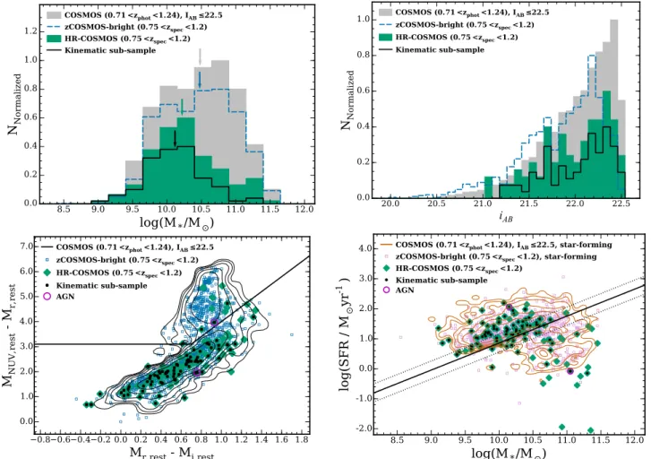
Fig. 2.Top panels: stellar mass (left) and IABselection magnitude (right) distributions of the 119 galaxies in our sample at 0.75 < z < 1.2 (green

histograms). We show for comparison the distributions of the parent samples in the same redshift range (COSMOS in gray and zCOSMOS-bright in blue) and in black the distribution of 82 galaxies in our kinematic sub-sample (see Sect.4.1). The photometric redshift range for the COSMOS sample takes into account the precision of the measurements (see text Sect.2.4). The arrows in the left panel show the median of each distribution. The histograms are re-normalized for a better visual comparison of their spreads and peaks, therefore their normalization does not reflect the actual scale. Bottom left panel: rest-frame MNUV− Mrversus Mr− MJcolor–color diagram. Colors are the same as in the top panels. The contours show

the distribution of the COSMOS parent sample with relative number of galaxies equal to 50%, 25%, 13%, 6%, 3%, 1.5% of the maximum of the distribution. The back solid line divides quiescent galaxies (above the line) from star-forming galaxies (below the line) and is determined following the technique adopted byIlbert et al.(2013). Bottom right panel: relationship between SED-derived star formation rate (SFR) and stellar mass. Green diamonds and black points represent the galaxies at 0.75 < z < 1.2 in our full sample and in our kinematic sub-sample, respectively. The dark-orange contours and the plum open squares show the distribution for the star-forming galaxies (as defined byLaigle et al. 2016) in COSMOS and zCOSMOS-bright samples, respectively. The contours represent the relative number of galaxies at the 50%, 25%, 13%, 6%, 3%, 1.5% of the maximum of the distribution. The solid and dotted lines represent the correlation, with the uncertainties, between the SFR and stellar mass of blue star-forming galaxies at 0.8 < z < 1.2 byElbaz et al.(2007). The magenta circles show the AGNs.

our sub-sample at z ∼ 0.75−1.2) using the HR redshift measure-ment, and we subtracted the stellar continuum spectrum, since we did not include it in the kinematic models (a cutout with continuum information was also saved for each observation). To perform the continuum subtraction we selected two background regions at the left and right of the emission line (avoiding reduc-tion artifacts and other spectral features), we stacked them, and we computed the median along the wavelength direction, ob-taining a spatial profile of the continuum that was subtracted for the entire cutout. During this process we visually inspected all the emission lines of the 119 galaxies in our sub-sample and we decided to discard 28 for which it would have been impossible to retrieve the kinematic information, either because the emis-sion line was too faint, or not detected, or it was shifted at the same wavelength of skylines (even if we selected galaxies with emission lines away from skylines, this could be possible for the targets selected with known photometric redshift for which the

measurements uncertainties are larger than for the spectroscopic redshift).

Although the slits were always carefully placed along the major axis of the galaxies (Sect. 2.2), we visually double-checked their correctness and we found that for one galaxy the slit was not well placed. The inclination, adopted for both the sample selection and the kinematic analysis, was also vi-sually inspected by overlapping ellipses with the axial ratio b/a from the Zurich Structure and Morphology Catalog on the HST/ACS F814W images of all the galaxies in our sub-sample (see Sect.A). During this visual inspection, we also found that one galaxy was obviously face-on, despite the fact that we se-lected galaxies with inclination&30◦_{(see Sect.2.1). Thus, these}

two galaxies (one with the slit misplaced and one face-one) were not included in our kinematic analysis. This reduced our sample to 89 galaxies, which have been modeled following the method described in Sect.3.

2.4. Stellar mass measurements

The stellar masses were estimated using the latest COSMOS photometric catalog (Laigle et al. 2016), which makes use of deep Spitzer SPASH IRAC imaging (Steinhardt et al. 2014) and the latest release of COSMOS UltraVISTA survey (McCracken et al. 2012). These measurements are extremely accurate since they are based on deep thirty-band UV–IR pho-tometry that covers all galaxy spectral types, and they were ob-tained using our high-resolution spectroscopic redshift measure-ments. The measurement technique follows the same recipes presented inIlbert et al.(2015), based on the Le Phare software (Arnouts et al. 2002;Ilbert et al. 2006). Briefly, the galaxy stel-lar masses have been derived using a library of synthetic spectra generated with the stellar population synthesis (SPS) package developed by Bruzual & Charlot (2003). We assume a univer-sal IMF fromChabrier(2003), as well as exponentially declin-ing and delayed star formation histories. For all these templates, two metallicities (solar and half-solar) are considered. Emission lines are added followingIlbert et al.(2009), and two attenuation curves are included: the starburst curve ofCalzetti et al.(2000) and a curve with a slope 0.9 (Appendix A ofArnouts et al. 2013). The stellar continuum extinction Es(B − V) is allowed to take

values in the range [0–0.7]. The values of the stellar masses were assigned using the median of the stellar mass probability distri-bution marginalized over all other parameters.

In Fig. 2, we show the distribution of various proper-ties of the HR-COSMOS sample of 119 galaxies in the red-shift range 0.75 < z < 1.2. These are contrasted with the parent zCOSMOS-bright and COSMOS samples. The values for both parent samples are drawn from the latest COSMOS photometric and SED-fitting catalogs (Laigle et al. 2016). For the former par-ent sample, we compare only those galaxies in the same spec-troscopic redshift range as the HR-COSMOS sample presented here. For the latter, the redshift range is extended slightly to 0.75 − 3σ_∆z/(1+zs)< z < 1.2 + 3σ∆z/(1+zs) to account for the un-certainties in the photometric redshifts, where σ_∆z/(1+zs)= 0.007. In the top panels, we present the stellar mass (left) and IABselection magnitude (right) distributions for our sample of

119 galaxies at 0.75 < z < 1.2 with green histograms and the distributions of the parent samples in gray (COSMOS) and blue (zCOSMOS-bright). Galaxies in our sample have stellar masses spanning from 1.3 × 109M to 2.0 × 1011 M and values of

IABspanning from 21.0 mag to 22.5 mag. The black histograms

show the distributions of the galaxies used in the kinematic analysis (see Sect. 4). Since we are not interested in compar-ing the normalization of the distributions, we re-normalized the histograms to better visually compare their spreads and peaks, therefore their normalization does not reflect the actual scale. We measure that the median of the parent samples distributions is equal to 3.0×1010_M

, while the median for the distribution of

our samples shifts to lower values (1.7 × 1010 Mfor the whole

sample of 119 galaxies and 1.3 × 1010 _M

for the kinematic

sub-sample). This may be a result of the fact that our sample is com-posed primarily of star-forming galaxies and, therefore, the high mass end of the parent samples distributions (probably populated by massive quiescent galaxies) is suppressed in our sample.

In the bottom panels of Fig. 2 we plot the rest-frame MNUV− Mr versus Mr− MJ color–color diagram (left) and the

relation between star formation rate (SFR) and stellar mass (right) for our sample compared to the parent samples. The color–color diagram is a diagnostic plot that enables us to sep-arate star-forming from quiescent galaxies. We divide quies-cent galaxies from star-forming galaxies following the technique

adopted by Ilbert et al. (2013). In the bottom left panel, we show how our sample follows the underling distribution of star-forming galaxies closely. This is supported by the SFR-M∗

re-lation displayed in the bottom right panel for the star-forming galaxies (as defined by Laigle et al. 2016) in COSMOS and zCOSMOS-bright samples. The SFR computed from SED fit-ting is known to be not as precise as that computed using other SFR estimators (Ilbert et al. 2015; Lee et al. 2015). Following Ilbert et al. (2015) we compared the SED-based SFR to the 24 µm IR SFR for the parent COSMOS sample in the redshift range 0.75 < z < 1.2, and found an offset of 0.15 dex towards larger SED-based SFR. To take into account this discrepancy, we applied a shift of −0.15 dex to the SFR measurements. Our sample follows the star-forming galaxy distribution of the parent samples.

3. Kinematic modeling

To study the galaxy kinematics, we created high-resolution semi-analytic models. The advantage of using a model to constrain the kinematics is that we can compare it directly to the observations, after taking into account all the degradation effects owing to the instrumental resolution, and avoid the intermediate steps of data analysis that can introduce additional noise (Fraternali & Binney 2006).

3.1. The model

Our first step for modeling the galaxy kinematics was to de-scribe an astrophysically-motivated picture of a galaxy at high-resolution. Ionized gas was described as rotating in a thin disc with a certain inclination i and position angle PA of the ma-jor axis. A pseudo-observation was created combining high-resolution models of intrinsic flux distribution of the emission line, rotation velocity and dispersion velocity using the follow-ing relation: I(r, V)= √Σ(r) 2πσ(r)exp ( −[V − V(r)] 2 2σ2_(r) ) · (1)

This models the galaxy emission at each radius r and recon-structs a 2D emission line to be compared to the observation. If the observed emission was a doublet (as in the case of [OII], the main investigated feature in this study) another contribution was added to the relation, having the same functional form and velocity dispersion σ as the previous one, but shifted in veloc-ity by a fixed value, that was equal to the separation between the two lines of the doublet, and scaled in intensity by a ra-tio R[OII], an additional parameter of the model. The intrinsic

line-flux distribution in the plane of the disc was described by a truncated exponential disc function:

Σ(r) =        Σ0e−r/r0 if r < rtrunc 0 if r > rtrunc , (2)

whereΣ0is the line flux at the center of the galaxy, r0is the scale

radius and rtruncis the maximum radius, after which the emission

is no longer detected. The truncation was necessary since we al-lowed r0to assume negative values to better match the observed

line flux distribution, in particular when the distribution is char-acterized by bright clumps in the peripheries of the galaxies.

The velocity along the line of sight, assuming that for spiral galaxies the expansion and the vertical motions are negligible

with respect to the rotation, was described as

V(r)= Vsys+ Vrot(r) sin i cos θ, (3)

where Vsys is the systemic velocity, that is the velocity

(cor-responding to the systemic redshift) of the entire galaxy with respect to our reference system. For very distant galaxies this quantity is usually dominated by the Hubble flow. Since we are interested only in the galaxy internal kinematics we set it to zero. The galaxy inclination i was measured as the angle between the line of sight and the normal to the plane of the galaxy (i= 0◦_for

face-on galaxy) and θ is the angle in the plane of the galaxy be-tween the galaxy PA and the position where the velocity is mea-sured. Since our model reproduces the emission coming from the slit aligned to the galaxy PA, we assume θ equal zero.

To model the rotation velocity Vrot, which results from both

baryonic (stars and gas) and dark matter potentials, three di ffer-ent functions have been used. All of them are described by two parameters: the maximum velocity Vt and the transition radius

rt. A velocity profile used is the Freeman disc (Freeman 1970),

which fits a galaxy with a gravitational potential generated by an exponential disc mass distribution. It is expressed as

Vrot(r)=

r h

p_πGµ

0h(I0K0− I1K1), (4)

where µ0 is the central surface density and h is the disc

scale-length of the surface density distribution. We note that µ0 and

hare not constrained byΣ0and r0 of Eq. (2) since the rotation

velocity model does not only describe baryons. Iiand Kiare the

i-order modified Bessel function evaluated at 0.5 r/h. The maxi-mum velocity

Vt∼ 0.88

p_πGµ

0h, (5)

is reached at the transition radius rt∼ 2.15h. Substituting Eq. (5)

and the transition radius rtin Eq. (4), we obtain an expression of

the rotation velocity Vrotdescribed by the only two parameters

Vtand rt. Unlike the Freeman disc, the two other rotation curve

models are analytic functions that have no physical derivation nor assumed mass distribution, but they appear to describe well the observed rotation curves of local galaxies. The flat model consists of a two slopes model, which describes a rotation veloc-ity distribution that has a sharp transition at rtand flats at Vt. It

takes the form: Vrot(r)=        Vt× r rt if r < rt Vt if r ≥ rt. (6)

Last velocity profile adopted is an arctangent function (Courteau 1997), expressed as Vrot(r)= Vt 2 πarctan 2r rt , (7)

which smoothly rises and reaches a maximum Vtasymptotically

at an infinite radius. The transition radius rtis defined as the

ra-dius for which the velocity is 70% of Vt. The galaxy velocity

dispersion σ has been modeled to be constant at each radius. This assumption is considered reasonable since it is based on what has been observed in the local Universe in the galaxies from the GHASP sample (Epinat et al. 2008). It has also been shown by some authors (Weiner et al. 2006b; Epinat et al. 2008) that the peak observed in the velocity dispersion profile for galaxies at high redshift is due to the blurring effect of the resolution. The high-resolution model sampling (both spectral and spatial)

was chosen to be a sub-multiple of the VIMOS data sampling. We therefore created high-resolution models with spectral and spatial sampling equal to 0.15 Å and 0.0512500_{, respectively. To}

make the high-resolution models comparable with the observa-tions, we performed a spatial and spectral smoothing by convolv-ing the models with the spatial resolution given by the seeconvolv-ing measured for each quadrant, and the spectral resolution of the instrument (see Sect.2.3). The effect due to the slit width was also taken into account by convolving the models with a win-dow function. Finally, the models were re-binned to match the VIMOS sampling (1 pixel= 0.20500_{= 0.6 Å).}

3.2. The fitting method

The comparison with the observation has been done through the χ2_{-minimization fitting using the Python routine MPFIT}

(Markwardt 2009), based on the Levenber-Marquardt least-squares technique. Preliminary steps were necessary to define a set of initial parameters.

The rotation center, rcenwas measured as the center of the

continuum spectrum’s spatial profile, or, when the continuum emission was too faint, as the center of the emission line’s spa-tial distribution around its observed central wavelength. This last quantity, λline(z), was a parameter of the model that was kept

fixed during the fitting process. Using our measured redshift (Sect.2.3) we derived the systemic velocity Vsys, which

quanti-fies the motion of the entire galaxy with respect to our reference system. However, for galaxies at high redshift Vsysis dominated

by the Hubble flow, therefore it is normal practice to set it to zero, to focus only on the internal kinematics. The systemic ve-locity is allowed to freely vary in the fitting to take into account the effect of the redshift measurement uncertainties. The incli-nation i is derived from the axial ratio, computed from HST im-ages, found in the literature (Zurich Structure and Morphology Catalog), and corrected for projection effects using Holmberg’s oblate spheroid description (Holmberg 1958):

i= arccos s (b/a)2− q2₀ 1 − q2 0 , (8)

where b/a is the observed axis ratio, q0= c/a is the axial ratio of

a galaxy viewed edge-on, a and b are the disc major and minor axes, and c is the polar axis. The value of q0 is known to vary

from 0.1 to 0.2 depending on galaxy type (Haynes & Giovanelli 1984). In this study we assumed q0 = 0.11, driven by the

ne-cessity to take into account the smallest value of b/a in our sample, that is 0.12, knowing form Pizagno et al. (2005) that the q0range 0.1−0.2 corresponds to a small variation (typically

∼1 km s−1 _{) in the velocity. Owing to the degeneracy between}

velocity and inclination (Begeman 1987) we decide to keep i fixed during the fit. The position angle PA is taken from the lit-erature and it is the same used to align the slit along the ma-jor axis of the galaxies during the observations (see Sect.2.2). The PA is fixed in the χ2 minimization fitting process. Al-though photometric-kinematic PA misalignment may exist, it has been demonstrated that PA measurements from high-resolution F814Wimages are generally in reasonable agreement with the kinematic PA.Epinat et al.(2009), for a sample of nine galaxies between 1.2 < z < 1.6 observed with SINFONI, found that the agreement between morphological and kinematic PA is better than 25◦, except for galaxies that have a morphology compati-ble with a galaxy seen face-on. A similar result was found by

-2.66 -1.84-1.02 0.0 0.82 1.64 2.46 _Data Model -2.66 -1.84-1.02 0.0 0.82 1.64 2.46 _Model Data 6900.08 6893.68 6886.7 6879.71 6872.73 6865.75 Wavelength ( ) -2.66 -1.84-1.02 0.0 0.82 1.64 2.46

Position along the major axis (arcsec)

6900.08 6894.26 6888.44 6882.62 6876.8 6870.98 6865.75

Wavelength ( )

Flux (counts)

Wavelength ( )

Flux (counts)

Position along the major axis (arcsec)

200 100 0 100 200

Velocity (km/s)

Fig. 3.Example of the output from the model-fitting process and the vision inspections to test the quality of the fit. Left panels: from top to bottom: continuum-subtracted 2D spectrum centered at [OII], best-fit kinematic model to the line emission, and residual image between the 2D spectrum and the best-fit model on the same intensity scale as the 2D spectrum. The vertical and horizontal axes are the spatial position and wavelength, respectively. In the first two panels, the black dot-dashed lines indicate the best-fit parameter rcen. In the top panel, the blue and red dotted lines

denote the positions from where the plots in the middle panels are extracted. The 2D spectrum from the VIMOS mask has been rotated to have always the North direction in the top. For this reason the wavelength direction is opposite to the conventional representation with values increasing (getting redder) towards left. The technique of tracing the emission line as a function of the position (see text Sect.3.2) is also shown in the top and middle pannels. Fuchsia circles show the central wavelength of the emission line at each position, and the green triangles show the centroids of the best-fit model. Middle panels: examples of the double Gaussian fit to measure the centroids of the emission line at two most external galaxy radii. Right panel: high-resolution rotation curve models (green line: exponential disc; red line: flat model; blue line: arctangent function), not corrected for the inclination, compared to the observed rotation curve (black circles). The errorbars on the y-axis direction represent the uncertainties of the fit to the line at each position to recover the centroid; the bars on the position direction indicate the bin size. The vertical dotted line indicates the galaxy rotation center, the horizontal dotted line indicates the systemic velocity, and the two vertical dashed lines indicates the position of the radius R2.2at which the velocity is measured to derive the scaling relations (Sect.4.1).

Wisnioski et al.(2015), who studied the galaxy kinematics of a sample of galaxies at 0.7 ≤ z ≤ 2.7 with KMOS, and have found that the agreement between photometric and kinematic PA is bet-ter than 15◦_{for 60% of the galaxies, and for 80% of the galaxies}

the agreement is better than 30◦, while misalignments greater than 30◦_{typically have axis ratios b/a> 0.6. In our sample only}

23 galaxies (out of 82) have b/a> 0.6.

The parameters that describe the rotation velocity Vtand rt,

the velocity dispersion σ, the doublet line flux ratio R[OII], and

the exponential disc truncation radius rtrunc have been guessed

tracing the continuum-subtracted emission line as a function of the spatial position. This procedure consists of fitting a Gaussian (double Gaussian with a rest-frame separation equal to 2.8 Å between the lines of the doublet) to the line profile in the length direction, and it returns the values of the central wave-length, the dispersion (both converted in velocities), and flux ra-tio (in case of doublet) in each spatial bin. The tracing procedure terminates when the emission is no longer detected above the local noise level (S /N < 3), and this gives us a guess on the pa-rameter rtrunc. Each trace has been visually inspected to ensure

that the fit was not influenced by spurious reduction artifacts. An example of this procedure is shown in Fig.3(middle panel). We defined the initial rotation velocity parameter Vt as the

av-erage value between the maximum velocities (corrected for the inclination) reached in both approaching and receding side of the galaxy and the transition radius rt as the average between

the radii at which the two maximum velocities have been first

reached. For the σ, since we decided to use a constant value, this was set as the mean over the traced dispersion, after correcting it for the instrumental dispersion followingWeiner et al.(2006b). The line flux ratio R[OII] has been defined as the mean over all

the line flux ratio values measured along every spatial bin. To recover the initial parameters that describe the surface brightness, we collapsed the emission line along the spectral direction (after subtracting the continuum), obtaining a spatial profile of the emission that has been fitted with a truncated ex-ponential disc (a sum of two truncated exex-ponential discs in case of a doublet) convolved with the spatial resolution. As a result, we get a first guess of the parametersΣ0and h. Except for the i,

PA and λline(z), the other parameters are let to vary freely in the

fitting process for a total of eight (nine, in the case of doublet) free parameters (Σ0, h, rtrunc, rcen, Vt, rt, Vsys, σ, R[OII]).

3.3. Uncertainty estimation of the parameters

The fits are done by minimizing the weighted difference be-tween the image of the 2D line emission and the 2D model of the same line. Each pixel is weighted by its inverse variance, which is computed by summing in quadrature the contribution from both the source and continuum-subtracted background. The first comes from the Poisson noise of the line-flux counts, and the second one is estimated directly from the rms fluctuation in regions where there is no object. These weights in the fit are translated into uncertainties on the parameters, computed from

1’’ ID831094 z=0.8972 1’’ z=0.9360 ID831493 1’’ z=0.9642 ID840437 1’’ z=0.8342 ID811920 1’’ z=0.9018 ID837931

Fig. 4.Examples of galaxies from our sample. For each galaxy we show the F814W HST/ACS postage stamp with superimposed the 100

width slit tilted to follow the galaxy major axis, the continuum-subtracted 2D spectrum, the best-fit kinematic model to the line emission and the residuals between the 2D spectrum and the best-fit model, on the same intensity scale as the 2D spectrum. In the spectra, the vertical and horizontal axes are the spatial position and wavelength, respectively. We show, both for the postage stamp and for the spectrum, the 100

scale. The first three galaxies are classified as rotation-dominated, whereas the other two galaxies are dispersion-dominated.

the covariance matrix. To the 1σ formal error from the fits, we added in quadrature to error on the parameter Vtthe

ties coming from the inclination (propagated from the uncertain-ties on b/a) and from the PA, since those parameters are kept fixed in the fitting process. The adopted b/a, from the Zurich Structure and Morphology Catalog, was measured with a soft-ware (GIM2D, see Sect.2.1), which gives morphological mea-surements that have been corrected for the instrumental point-spread function (PSF). In Sect.A, we computed systematic un-certainties on the measurements of the axial ratio b/a derived by small variation of the PSF and added them to the velocity error budget. We measured the instrumental resolution from the sky-lines (see Sect.2.3) and we found that it varies from 2.58 Å to 3.20 Å with a distribution that peaks at 2.63 Å. Since we con-structed our model using the nominal spectral resolution (3 Å) of the instrument, we adjusted the value of the parameter σ by applying a resolution correction using the value of the peak of the spectral FWHM distribution 2.63 Å, and then we added the dispersion of the distribution to the uncertainties on σ. In me-dian, we added −0.8 km s−1and+4.7 km s−1to the formal error on σ from the fit.

4. Results

4.1. Kinematic parameters

The Levenberg-Marquardt least-squares fitting method is known to be sensitive to the local minima, thus it is important to choose the initial guesses as being as close as possible to the global minima. We accounted for this by measuring the initial guesses as described in Sect.3.2. Furthermore, to explore the effect of the initial guesses on the resultant models, we adopted a Monte Carlo approach, which consists of perturbing the initial guesses by sampling a Gaussian distribution, obtaining 500 combina-tions of the free parameters and running the fit for every single combination. Amongst the fits that converged to a best-fit solu-tion, we discarded the ones that have obviously wrong values for the parameters and extremely high values of the parameter errors, and we pre-selected the best-fit solutions in the lowest range of χ2(within the 10% of the lowest value). We then defined the best-fit model as the solution with the value of the parame-ter Vtappeared most frequently at the most frequent χ2value in

the pre-selected χ2distribution. Our results do not change if we, instead, define the best-fit model as the solution with the most

z=0.8676 ID834100 z=0.8248 ID837355 z=1.121 ID833209 z=0.9351 ID817416 ID819479 z=0.7505 z=0.7613 ID813055 z=1.1774 ID826042 z=0.9711 ID833167 z=0.850 ID830321 z=0.9234 ID830414 z=0.9018 ID837931 z=1.1694 ID701403 z=0.8383 ID811012 z=0.8342 ID811920 z=0.8742 ID818734 z=0.7684 ID813411

Fig. 5.F814WHST/ACS postage stamps of our sub-sample of dispersion-dominated galaxies, with superimposed the 100

width slit tilted to follow the galaxy major axis.

frequently occurring value of the parameter Vt within the

pre-selected χ2distribution.

In this way, we obtained one best solution (when available) for each modeled rotation curve (exponential disc, flat model and arctangent function). For each galaxy, we visually inspected their residual images, the trace of the emission at each position (see Sect.3.2) – both for the observed spectrum and the modeled one – and their rotation curves (see Fig.3). In general we chose the exponential disc solution, if available, by default. For our sample 60% of the galaxies were modeled by an exponential disc rota-tion curve. If the exponential disc solurota-tion was not available, we adopted the flat model solution and, if not available, the arctan-gent function solution. This decision was motivated by the fact that for the 50% of the sample, for which we got successfully a best-fit solution for each rotation curve model, the velocity V2.2,

that is the velocity used to derive the scaling relations (see later in this subsection), was always consistent within the uncertain-ties for all the rotation curve solutions.

The χ2-minimization fitting was run for 89 galaxies. Al-though seven of these presented noisy spectra (S /N < 3), the fitting was attempted. However, from our visual check we found that no best-fit parameters could properly reproduce the obser-vations, so we discarded them, which resulted in a final sample

of 82 galaxies. Examples of ours spectral data and best-fit model are shown in Fig.4.

To retrieve galaxy scaling relations and the dynamical masses, it is important to choose a fiducial radius at which the rotation velocity is measured. Past studies have shown that using different kinematic estimators (e.g., the maximal rotation veloc-ity Vmax, the plateau rotation curve velocity Vflat, the velocity

V80 measured at the radius containing ∼80% of the total light,

and the velocity V2.2 measured at R2.2 = 2.2 Rd, where Rd is

the disc scale-length estimated from broad band imaging) can lead to different results (see, e.g.,Verheijen 2001;Pizagno et al. 2007). In our sample, we adopted the V2.2estimator, which

pro-vides the tightest scatter in various galaxy scaling relations for bright galaxies and the best match to radio (21 cm) line widths for local galaxies (Courteau 1997). The values of R2.2are

com-puted as 2.2 times the galaxy disc scale length measured from the HST/ACS F814W images (Scarlata et al. 2007) and included in the Zurich Structure and Morphology Catalog.

The model is not always able to reproduce the surface bright-ness profile of the observation, since a few discs are likely to be well described by an exponential profile, especially at high red-shift, where a considerable number of galaxies shows clumpy star formation (Förster Schreiber et al. 2009;Wuyts et al. 2012).

We tested the reliability of rotation velocity parameters obtained from the fitting to the models by creating mock observations of galaxies (including the contribution of the background noise) with known rotation velocity and with diverse surface brightness profiles (generally described as a sum of two exponential func-tions with different Σ0, r0 and rcen) and we fitted them with our

models, assuming an exponential disc surface brightness. We ob-tained that the values of the velocity best-fit parameters with dif-ferent surface brightness profiles were always consistent within 1σ errors. We also tested (see AppendixB) the correctness of the assumption of an exponential disc profile on the real data, by using an algorithm fromScoville et al.(1983; see Sect. 3 therein for a detailed description) to derive the high-resolution spatial distribution of the galaxy emission that best matches the ob-served emission line profile shape. Including the profile derived in this way and re-fitting to the data, we found that the rotation velocity parameters were not affected by adopting this surface brightness profile.

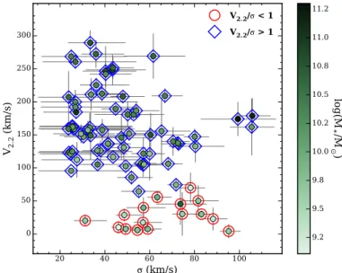
The kinematic parameters of our sample are listed in Table E.1. We found that in 82 successful fits, 66 galaxies (80%) are formally rotation-dominated and 16 galaxies (20%) are dispersion-dominated, by V2.2/σ > 1 and V2.2/σ < 1,

re-spectively. We present in Fig.5HST/ACS images of our sample of dispersion-dominated galaxies. In Fig.6we show a correla-tion between V2.2and σ for dispersion-dominated and

rotation-dominated galaxies. Each point in Fig.6is color–coded accord-ing to its stellar mass and we can see that the most massive galaxies amongst the rotation-dominated ones have the largest values of V2.2. A similar result was found byEpinat et al.(2009),

who have studied the kinematics of a sample of star-forming galaxies at 1.2 < z < 1.6. This would imply that the most mas-sive star-forming galaxies are the most kinematically settled. Same result was presented byKassin et al.(2012), who studied the internal kinematics of 544 so called blue galaxies with stel-lar masses ranging 8.0 < log M∗(M) < 10.7 over 0.2 < z < 1.2,

and found the most massive galaxies being the most evolved at any time. Another study fromSimons et al.(2015) reports a tran-sition mass in the smTF relation, log M∗(M)= 9.5, which they

call the “mass of disc formation” Mdf, for a sample of

emis-sion line galaxies at 0.1 < z < 0.375. This mass separates the galaxies that always form discs (M∗> Mdf) and are settled on

to the local smTF relation, from those which may or may not form discs (M∗< Mdf) and can either lie on the smTF relation

or scatter off of it to low rotation velocity and higher disordered motions. We are aware, however, that the characterization of a galaxy as dispersion or rotatation-dominated is a strong func-tion of the galaxy size. Newman et al. (2013b) compared the kinematic analysis of a sample of 81 star-forming galaxies at z= 1.0−2.5 using IFU data observed with both seeing-limited and adaptive optics (AO) mode, and found that small galaxies are more likely to fall in the category of dispersion-dominated galaxies because of either insufficiently resolved rotation (es-pecially with seeing-limited observations) or as a result of the almost constant values of velocity dispersion across all galaxy sizes while the values of rotation velocity linearly increase with size. They also found that many galaxies, which were considered dispersion-dominated from more poorly resolved data, actually showed evidence for rotation in higher resolution data but, in spite of this, they found that those galaxies have different av-erage properties than rotation-dominated galaxies. They tend to have lower stellar and dynamical masses, higher gas fractions, younger ages, and slightly lower metallicities. They suggest that these galaxies could be precursors of larger rotating galaxies, as they accrete more mass onto the outer regions of their discs.

Fig. 6.Rotation velocity V2.2as a function of the velocity dispersion σ.

The points are color–coded according their stellar mass. Blue and red circles around the points identify rotation- and dispersion-dominated galaxies, respectively.

We investigated any possible correlation between the size of the galaxies and the measured V2.2/σ, by estimating the fraction

of galaxies that have the radius r80, defined as the semi-major

axis length of an ellipse encompassing 80% of total light (from the Zurich Structure and Morphology Catalog), smaller than the measured seeing (Sect. 2.3). We found that this condition was true for 80% of the dispersion-dominated galaxies, while 60% of the total sample have r80 smaller than the seeing. Therefore,

although r80is only an approximation for the size of the galaxy,

we found that the fraction of dispersion-dominated galaxies with small size is over-represented compared to the total fraction, sug-gesting that the classification as dispersion-dominated may be biased by the size of the galaxies.

We compared our kinematic classification to the galaxy mor-phologies as measured from the HST images byScarlata et al. (2007), and we found that half of the dispersion-dominated sam-ple is formed by galaxies defined as irregular, while 31% have an intermediate bulge and only three galaxies (19%) are classified as pure discs. The majority of the rotation-dominated galaxies, instead, are constituted of pure discs (42%), while 29% are formed by galaxies with intermediate bulge and 23% are de-fined as irregular. The remaining 6% is formed by three bulge-dominated galaxies and one early type. Three galaxies in Fig.6 do not follow the correlation and, even though they rotate quite fast, they exhibit high velocity dispersion. For the two most mas-sive galaxies a clear presence of a prominent bulge in the HST images, or unresolved inner velocity gradient not described by simple models or intrinsic dispersion, may be the cause of the high dispersion, even though their discs are still rotating. The less massive one has a bright clumpy region in the periphery, which may have high dispersion and which, due to its relatively high brightness, may dominate the emission.

Most of our kinematic sample is composed of [OII] emission line galaxies (79 out of 82) and, for those galaxies, we measured the line ratio R[OII]from the model fitting. We show the

distribu-tion of R[OII] along with its relationship to other galaxy

param-eters (σ, M∗, SFR) in AppendixC. We measured the rest-frame

equivalent width (EW) and computed the SFR from [OII] fol-lowingLemaux et al.(2014). The choice of using EW([OII]) to

0.5

1.0

1.5

2.0

2.5

log(V

_2.2

/kms

-1

₎

8.5

9.0

9.5

10.0

10.5

11.0

11.5

lo

g(

M

*

/M

)

slope =3.683 ±0.787

intercept =2.154 ±0.147

=0.106

rms

=0.116

z=0 Pizagno et al 2005 (N=81)

z~0.6 Puech et al 2008 (N=16)

z=0.8-1.25 Miller et al 2011 (N=37)

z=0.75-1.2 This work (N=64)

AGN

Fig. 7.SmTF relation constrained for our sample of rotation-dominated galaxies (black circles). The gray points are the dispersion-dominated galaxies. The magenta stars show the AGNs. Our fit is represented with a solid red line. The dotted red lines show the intrinsic scatter σintr. We

plot as references the relations at z= 0 (Pizagno et al. 2005) with a short-dashed black line, z ∼ 0.6 (Puech et al. 2008) with a dot-dashed green line and z= 0.8–1.25 (Miller et al. 2011) with a long-dashed blue line.

derive the SFR instead of [OII] flux was motivated by the lack of the absolute flux calibration for our spectroscopic observations (see Sect. 2.3). In Fig. C.4 we show the comparison between the SFR computed using the spectral energy distribution (SED) fitting and the [OII] emission. The values of R[OII], SFRSEDand

SFR[OII]are listed in TableE.2.

4.2. Stellar mass Tully-Fisher relation at z ∼ 0.9

We present the stellar mass Tully-Fisher (smTF) relation ob-tained at z ∼ 0.9 in the COSMOS field. This is shown in Fig.7 and takes the form:

log M∗= a (log V2.2− log V2.2,0)+ b , (9)

where a and b are the slope and the y-intercept of the rela-tion, respectively, and log V2.2,0is chosen to be equal to 2.0 dex

to minimize the correlation between the errors on a and b (Tremaine et al. 2002). Since the smTF relation is known to be valid for rotating galaxies, we decided to fit the relation for the rotation-dominated sub-sample, shown in Fig.7with black cir-cles, whereas the dispersion-dominated galaxies are plotted as gray points. We decided not to include the two galaxies known to be NL AGNs in the fit of the smTF relation, since we can-not tell if the emission is dominated by the AGN or by the host. We note that, for those galaxies, the stellar mass measure-ments may not be correct since AGNs were not taken into ac-count in the SED-fitting process. The relation in Eq. (9) is ob-tained using MPFITEXY routine (Williams et al. 2010), which

adopts a least-squares approach accounting for the uncertainties in both coordinates and incorporates the measurement of the in-trinsic scatter σintron the velocity variable, added in quadrature

to the overall error budget. The MPFITEXY routine depends on the MPFIT package (Markwardt 2009). Following previous analyses of the Tully-Fisher relation (see e.g.,Verheijen 2001; Pizagno et al. 2005,2007;Miller et al. 2011;Reyes et al. 2011), we fitted an inverse linear regression to our data, where velocity is treated as the dependent variable. The relation is then inverted to compare the fitted parameters to other works, which show the forwardbest-fit parameters of the smTF relation. MPFITEXY automatically handles the inversion of the results and the prop-agation of errors. Forward and Inverse fitting is only symmetric if there is no intrinsic scatter (σintr = 0) (Tremaine et al. 2002),

but generally this is not the case. It has been shown in previ-ous works (e.g.,Willick 1994;Weiner et al. 2006a) that there is a significant bias in the slope of the forward best fit relation in-troduced by the sample selection limits. Therefore the inverse relationship is usually preferred, where the galaxy parameters that are more subject to the selection effects (magnitude, stellar mass) are treated as the independent variable.

We determined the 1σ errors on a, and b, by repeating the fit for 100 bootstrap sub-samples of 82 galaxies from the full rotation-dominated galaxy sample and taking the dispersion of the distribution of bootstrap estimated parameters as the uncer-tainty in the same parameters. Our best-fit parameters are shown in Table2.

To investigate the evolution of the smTF relation with red-shift, we plotted the relations at z= 0 fromPizagno et al.(2005)