Brandt's GLR method & refined HMM segmentation for TTS synthesis application

HAL Id: hal-02137832

https://hal.archives-ouvertes.fr/hal-02137832

Submitted on 23 May 2019

HAL is a multi-disciplinary open access

archive for the deposit and dissemination of

sci-entific research documents, whether they are

pub-lished or not. The documents may come from

teaching and research institutions in France or

abroad, or from public or private research centers.

L’archive ouverte pluridisciplinaire HAL, est

destinée au dépôt et à la diffusion de documents

scientifiques de niveau recherche, publiés ou non,

émanant des établissements d’enseignement et de

recherche français ou étrangers, des laboratoires

publics ou privés.

Brandt’s GLR method & refined HMM segmentation for

TTS synthesis application

Safaa Jarifi, Dominique Pastor, Olivier Rosec

To cite this version:

Safaa Jarifi, Dominique Pastor, Olivier Rosec. Brandt’s GLR method & refined HMM segmentation

for TTS synthesis application. EUSIPCO’05 : 13th European Signal Processing Conference, Sep 2005,

Antalya, Turkey. �hal-02137832�

Safaa Jarifi*, Dominique Pastor*, Olivier Rosec**

T´el´ecommunications de Bretagne, Technopˆole Brest Iroise, 29238 Brest Cedex, France

safaa.jarifi, [email protected]

** France Telecom, R&D Division TECH/SSTP/VMI 2, avenue Pierre Marzin, 22307 Lannion Cedex

[email protected]

ABSTRACT

In comparison with standard HMM (Hidden Markov Model) with forced alignment, this paper discusses two automatic segmentation algorithms from different points of view: the probabilities of insertion and omission, and the accuracy. The first algorithm, hereafter named the refined HMM algo-rithm, aims at refining the segmentation performed by stan-dard HMM via a GMM (Gaussian Mixture Model) of each boundary. The second is the Brandt’s GLR (Generalized Likelihood Ratio) method. Its goal is to detect signal dis-continuities. Provided that the sequence of speech units is known, the experimental results presented in this paper sug-gest in combining the refined HMM algorithm with Brandt’s GLR method and other algorithms adapted to the detection of boundaries between known acoustic classes.

1. INTRODUCTION

The objective of this paper is the segmentation of large acoustic databases for application to corpus-based speech synthesis. Segmenting spontaneous and continuous speech signals is still an issue. Because the sequence of speech units is known, automatic segmentation is usually performed by HMM’s with forced alignment. This procedure shows rea-sonable results. However, in order to guarantee a good qual-ity of a synthetic voice, the outcome of the segmentation stage must still be verified manually, which is a difficult task. Thus, it is still important to design a segmentation algorithm capable of providing segmentation marks close to handmade ones with the smallest possible number of errors.

With respect to the foregoing, the purpose of this paper is to analyze and compare the accuracies of three segmentation algorithms on a large French corpus. The first one is the stan-dard HMM with forced alignment as described above. The second one is the refined HMM, originally proposed in [7] for segmenting a Chinese corpus. These two methods lead to a number of segmentation marks that corresponds to the number of phonemes in the input speech unit sequence. Thus they do not yield omissions nor insertions. The third algo-rithm is Brandt’s GLR method ([2]) which aims at detecting discontinuities of speech signals without any further knowl-edge upon the phonetic sequence. As this algorithm is lin-guistically unconstrained, it makes insertions and omissions. From this comparison, we derive an approach aimed at improving the accuracy of the refined HMM so as to tend to some reasonable performance objective introduced below.

The paper is organized as follows. In the next two sec-tions, we briefly present the refined HMM and Brandt’s GLR THIS STUDY IS SUPPORTED BY THE R&D DIVISION OF FRANCE TELECOM.

method. After introducing how performance measurements are computed, section 4 presents and discusses experimental results. On the basis of these results, we suggest in section 5 an approach for improving the refined HMM.

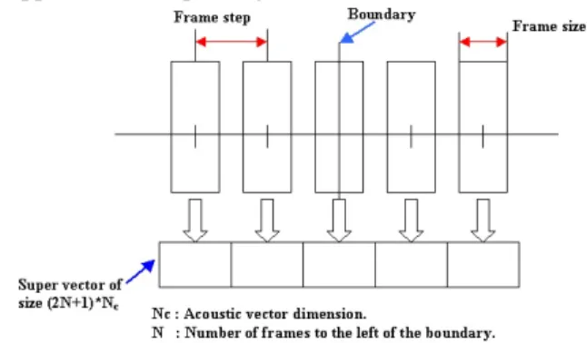
Figure 1: Example of a super vector for a particular boundary

2. THE REFINED HMM ALGORITHM

The main idea of this method is to train a GMM model for each HMM boundary with super vectors that are extracted using frames around the boundaries ([7, 5]). This method is carried out in three steps:

1. Achieve an HMM segmentation with forced alignment. Thus, the number of segmentation marks equals that of the handmade segmentation.

2. For a small database that is manually segmented, create a super vector for each boundary of this database. This vector is obtained by putting together acoustic vectors for frames near the boundary. In Fig. 1, we illustrate a super vector with (2N + 1) frames.

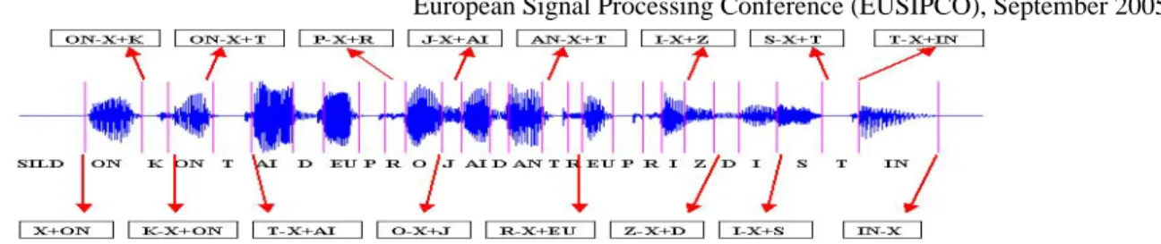
Each boundary B depends on the phoneme X to the left of it and on the phoneme Y to its right. We denote this boundary by X − B + Y as proposed in [8] (see Fig. 2). If we model each possible pseudo triphone by a GMM, the models are badly trained. This is because the num-ber of labeled data is limited in practice. Therefore, a classification and regression tree (CART) is used in or-der to cluster pseudo-triphones into a reduced number of classes; this cart is a recursive binary tree where each node corresponds to a phonemic or linguistic question. Then a GMM is trained for each leaf node on the CART. 3. Given a labeled sentence and its segmentation, try to re-fine each boundary of every segment. In this respect, for each frame in a certain vicinity of a given HMM bound-ary, compute the likelihood that this frame contains the actual boundary. The likelihood that the true boundary 1

Figure 2: Examples of pseudo-triphones lies within a given frame is then computed as follows.

We form a super vector centered on the current frame. Since this super vector is assumed to represent a pseudo-triphone, we determine the corresponding leaf node in the CART. We then compute the likelihood of the GMM model associated with this leaf node. Finally, the optimal boundary is then assumed to be in the frame that has the maximum likelihood.

3. BRANDT’S GLR METHOD

The aim of this method is to detect discontinuities in speech signals. Speech signals are assumed to be sequences of ho-mogeneous units. Each unit or window w is a finite sequence

w = (yn) of samples that are assumed to obey an AR model:

yn=∑_i=1p aiyn−i+ en. In this equation, p is the model

or-der, which is assumed to be constant for all units and en

is a zero mean white gaussian noise with variance equal to

σ2. Such a unit is thus characterized by the parameter vector

Θ= (a1, . . . , ap, σ ). Let w0be some window of n samples andΘ0the corresponding parameter vector. Brandt attempts in [2] to decide whether w0should be split in two subseg-ments w1and w2or not. In fact, a possible splitting derives from the detection of some jump between the parameter vec-tors Θ1 and Θ2 of w1 and w2 respectively. Brandt’s GLR method decides that such a jump has occurred by compar-ing: Dn(r) = nlog ˆσ0− rlog ˆσ1− (n − r)log ˆσ2to a predefined threshold λ . Note that Dnis merely the GLR. In the

equa-tion above, r is the size of the time interval covered by w1, whereas ˆσ1and ˆσ2are the noise standard deviation estimates of the models characterized respectively by the parameter vectors Θ1 and Θ2. Thus, the change instant corresponds to arg(maxr(Dn(r)) ≥ λ ).

A direct implementation of this method is computation-ally expensive. Thus, we use the sub-optimal version recom-mended in [7]. In particular, the length of w2is fixed to a predefined value L. For further details, the reader can refer to [2, 3].

4. EXPERIMENTAL RESULTS AND DISCUSSION

Our purpose is to analyze the behavior of the algorithms pre-sented above. We do so by computing performance measure-ments on the basis of experimeasure-ments. We start by describing the criteria used to evaluate the performance of each algo-rithm. These performance criteria are the probabilities of in-sertion and omission and the accuracy. On the basis of [7], we then adjust the refined HMM parameters for application to a French corpus. For this tuning, only the accuracy is needed because the refined HMM yields no insertions and no omissions. For Brandt’s GLR method, we compute the probabilities of insertion and omission. The last subsection compares the accuracies of the refined HMM, the standard HMM and Brandt’s GLR method.

4.1 Probabilities of insertion and omission, accuracies

The quantities described in this section allow us to measure the performance of any segmentation algorithm. We pro-pose the subsequent definitions especially in order to take into account insertions and omissions of algorithms such as Brandt’s GLR method.

We start by briefly describing how to locate insertions and omissions of a segmentation algorithm so as to compute the probabilities of insertion and omission of this same algo-rithm.

Let U = {U1,U2, . . . ,Un} and V = {V1,V2, . . . ,Vp} be the

time instants of the segmentation marks obtained respec-tively by an automatic algorithm and by a manual procedure (hereon referred to as the reference segmentation). For each

Uj, a correspondence is done with the reference

segmenta-tion by determining the time instant Vkj which is closest to

Uj. This way, a sequence VU= {Vk1, . . . ,Vkn} is built in order to compare both segmentation.

The reader can easily verify the following facts: the omissions are the marks V`, ` ∈ {1, . . . , p}, that are not in

the list VU; if VU contains m times the same mark, the

num-ber of insertions niequals m − 1. In the latter case, if V`is the

mark contained m times in the list VU, the nearest mark to V`

in U is considered as a non-insertion and, thence, the m − 1 other marks are regarded as insertions.

We define the ratios Pi= p+nnii and Po= no

n+no. The for-mer can be regarded as the probability of insertion of the segmentation algorithm, whereas the latter can be consid-ered as the probability of omission of this algorithm. Note that n + no= p + ni.

The accuracy of any given segmentation is computed as follows. First, locate the insertions as described above and remove them from the list U . For each mark Uj of the

re-sulting list of non-insertions, consider the closest reference mark Vkj. If the distance |Vkj− Uj| is less than or equal to a given tolerance value ε, the mark segmentation Uj is said

to be correct. Otherwise, it is called an error. The accuracy is then defined as the ratio in percentage of the number of correct marks to p + ni: accuracy = 100 p + ni n

∑

where I_[0,ε](x) equals 1 if x ∈ [0, ε] and 0 otherwise. The

accuracy depends on the number of insertions, the number of omissions and ε. Therefore, an accurate segmentation must make a good compromise between these three parameters.

For instance, a segmentation with many insertions will clearly be characterized by a Pi close to 1 and an accuracy

close to 0; similarly, in the case of many omissions, Po is

close to 1 and the accuracy remains small; in contrast with 2

are small and the accuracy is close to 1. Further mathematical details regarding these criteria will be given in a forthcoming work.

4.2 Application of the refined HMM algorithm to a French corpus

As mentioned in [7], the method “makes no inherent assump-tions for the language or speaker type”. So, our purpose is to validate the parameter values exhibited in [7] when we apply the method to a French corpus containing 7350 sentences. We also adjust some parameters in addition to the reference. We proceed by using HTK toolkits [8]. Note that the notion of accuracy used in [7] is a particular case of that employed in this present paper to measure the performance of segmen-tation algorithms.

The training parameters of this algorithm are: the train-ing size, the number of frames (2N + 1), the frame step e, the frame size (set to 20 ms), the number of GMM components (equal to 1, see [7] for details), the acoustic vector dimension

Nc(set to 39 : 12 MFCCs+ energy+ 13 first order deviations+

13 secondary deviations), the stopping criteria of the CART. These are the minimum number of leaf node instances, de-noted by MT I, and the value T of the log likelihood to ex-ceed, in order to consider a question as an actual node of the CART. For every HMM mark of the database, the refined HMM boundary is searched within a 60 ms interval centered on this mark with a search step fixed to 5 ms. The accuracies presented below are calculated for ε equal to 5, 10, 20 and 30 ms. They must be compared to those obtained by standard HMM and given in table 1.

In table 2, we point out a suitable pair (T, MT I) that yields a good level of accuracy when the tolerance varies. The results of table 2 are obtained by following [7] and thus fixing the pair (N, e) to (2, 30) and the training size to 300. We observe that T hardly influences the accuracy. We fix T to 100. The results also show that the smaller the MT I, the better the accuracy.

Table 3 illustrates the contribution of the training database size. We again fix the pair (N, e) to (2, 30). The pair

(T, MT I) is set to (100, 10) according to the foregoing. On

the basis of these results, we choose a size of 300 sentences in order to limit the number of manually labeled boundaries. This value is close to that obtained for a Chinese corpus in [7] With table 4, we verify that (N, e) = (2, 30) still remains a suitable choice for dealing with our French corpus. In fact, this choice seems to be a reasonable trade-off between the following two facts. On the one hand, the total duration cor-responding to the super vector must be long enough to in-volve as much information as possible concerning the tran-sition between the two phonemes around the boundary. On the other hand, if this duration is too long, the super vector will take into account information not directly linked to the boundary itself.

Summarizing, the refined HMM algorithm performs well when applied to a French corpus (6% accuracy gain when the tolerance is 10 ms) with MT I = 10, N = 2, e = 30 ms and a training size equal to 300.

20 87.91 87.74 87.05 85.16 30 94.46 94.44 93.93 93.45 5 38.55 38.12 37.48 35.13 100 10 64.63 64.28 62.94 60.13 20 87.98 87.73 87.04 85.16 30 94.50 94.46 93.93 93.45 5 38.38 37.90 37.49 35.13 350 10 64.32 64.01 62.94 60.13 20 87.93 87.51 87.11 85.16 30 94.35 94.42 93.93 93.45

Table 3: Accuracy vs training set size

Training size ε = 5 ε = 10 ε = 20 ε = 30

200 38.27 63.97 87.63 94.31

300 38.55 64.63 87.98 94.49

600 41.26 67.10 88.78 95.03

800 41.42 67.76 88.87 95.15

4.3 Insertions and omissions with Brandt’s GLR method

For Brandt’s GLR method, the model order p and the win-dow length L are chosen equal to 16 and 20 ms respectively. The threshold λ is set to 30 as in [3].

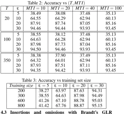
We found that the probabilities of insertion and omis-sion are equal to 0.6 and 0.1 respectively. This high inser-tion probability is explained by the oscillatory behavior of the GLR function. Note that the insertion probability is di-vided by two when the Brandt’GLR method is merged with a silence/speech detection [1]. Indeed, many insertions are located in silences (see Figure 3).

4.4 Comparing the accuracies of the refined HMM and Brandt’s GLR methods

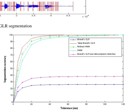
The results presented in this section are obtained by averag-ing the accuracies usaverag-ing a cross-validation procedure where each test set contains 1200 sentences. For the refined HMM, the training set contains 300 sentences for each test. Figure 4 depicts the results obtained with the three methods. Note that for Brandt’s GLR method three curves are plotted. The “Brandt’s GLR” curve represents the accuracies of this al-gorithm taking into account its insertions and omissions; the “Brandt’s GLR and speech/silence detection” curve displays the accuracies when Brandt’s GLR method is merged with the speech/silence detection algorithm already used in [1]; the “ideal Brandt’s GLR” curve is obtained by computing accuracies after removing the insertions and omissions via the procedure of subsection 4.1.

According to the results illustrated by these curves, we can make the following remarks: the refined HMM is more accurate than the standard HMM segmentation; the Brandt’s GLR method is not accurate because of its large number

Table 4: Accuracies for different values of (N, e)

e N ε = 5 ε = 10 ε = 20 ε = 30 0 0 33.95 58.70 83.70 92.27 10 2 39.01 64.42 86.13 93.41 30 2 38.55 64.63 87.98 94.49 30 3 37.16 63.83 88.06 94.58 3

Figure 3: Brandt’s GLR segmentation of insertions even when this number of insertions is

signifi-cantly reduced; the accuracy of the “ideal” Brandt segmenta-tion is itself significantly better than that of the refined HMM. Therefore, the marks produced by Brandt’s GLR method that are not insertions are more accurate than those of the refined HMM.

5. SUGGESTIONS FOR IMPROVING THE REFINED HMM

As mentioned above, Brandt’s GLR method is not accu-rate with respect to the accuracy measure given in this pa-per. It is however worth noticing that our assessment is too strict regarding Brandt’s GLR method because the defini-tion of accuracy does not take into account the distribudefini-tion of segmentation marks. In fact, insertions of Brandt’s GLR method remain located in silence regions and in the vicinity of handmade marks. It also turns out that high values of the GLR correspond to actual discontinuities of speech signals. Hence, we suggest to improve the accuracy of the refined HMM by proceeding as follows.

Given a segmentation mark performed by the refined HMM algorithm, compute the GLR of this initial mark. If the GLR exceeds some threshold (to define), keep this mark. Otherwise, consider that neither the refined HMM nor Brandt’s GLR method are reliable. Therefore, choose a seg-mentation algorithm adapted to the acoustic classes of the segments to identify. These classes are known thanks to the sequence of speech units we have. Basic examples of such algorithms are speech/silence detection and voiced/unvoiced detection. More sophisticated techniques are described in the literature on the topic (see for instance [6]).

Since Brandt’s algorithm segmentation marks that are not insertions are accurate, it can easily be thought up that a reasonable performance objective for the approach described above is to achieve accuracies better than those of the refined HMM and closer to those of the “ideal” Brandt segmentation.

6. CONCLUSION

This paper analyzed the performance measurements of two automatic segmentation algorithms: the refined HMM algo-rithm and Brandt’s GLR method. To carry out our assess-ment, we used three performance criteria, namely, the prob-ability of insertion, the probprob-ability of omission and the accu-racy. From the experimental results, we derived an approach for improving the refined HMM segmentation algorithm as well as a reasonable performance target (the accuracy of the “ideal” Brandt’s GLR method). With respect to the contents of this paper, the purpose of our forthcoming work will be twofold. On the one hand, we will complete our analysis con-cerning the performance criteria. In particular, we will study how the distribution of marks can be taken into account or merged with the criteria employed in this paper. On the other hand, we will detail, implement and test the method proposed

Figure 4: Segmentation accuracy for 900 sentences in the foregoing section. Our intention is to approach the ac-curacy of the “ideal” Brandt segmentation.

REFERENCES

[1] S. Jarifi, D. Pastor, O. Rosec, Jump and silence/speech

detection for automatic continuous speech segmentation,

International Symposium on Image/Video Communica-tions, Brest, France, 2004.

[2] R.A. Obrecht, Automatic segmentation of continuous speech signals, Proc, ICASSP, pp.2275-2278, Tokyo,

Japan, 1986.

[3] R.A. Obrecht, A New Statistical Approach for the

Au-tomatic Segmentation of Continuous Speech Signals ,

IEEE Transactions on Acoustics, Speech and Signal Pro-cessing, Vol.36(1), pp.29-40, 1988.

[4] M. Seck, D´etection de ruptures et suivi de classe de

sons pour l’indexation sonore, Phd thesis, Universit´e de

Rennes 1, France, 2001.

[5] A. Sethy and S. Narayanan, Refined Speech

Segmenta-tion for Concatenative Speech Synthesis, Proc, ICSLP,

pp.149-152, Denver, USA, 2002.

[6] D.T. Toledano and L.A. Hern´andez G´omez and L. Vil-larubia Grande, Automatic Phonetic Segmentation,

IEEE Transactions on Speech and Audio Processing, Vol.11(6), pp.617-625, 2003.

[7] L. Wang and Y. Zhao and M. Chu and J. Zhou and Z. Cao, Refining Segmental Boundaries for TTS Database Using Fine Contextual-Dependent Boudary Models, Proc. ICASSP, pp.641-644, Montreal, Canada,

2004.

[8] S. Young and G. Evermann and T. Hain and D. Kershow and G. Moore and J. Odell, The HTK Book for HTK

V3.2.1 , Cambridge University Press, Cambridge, 2002.