HAL Id: hal-00317385
https://hal.archives-ouvertes.fr/hal-00317385
Submitted on 1 Jan 2002
HAL is a multi-disciplinary open access
archive for the deposit and dissemination of
sci-entific research documents, whether they are
pub-lished or not. The documents may come from
teaching and research institutions in France or
abroad, or from public or private research centers.
L’archive ouverte pluridisciplinaire HAL, est
destinée au dépôt et à la diffusion de documents
scientifiques de niveau recherche, publiés ou non,
émanant des établissements d’enseignement et de
recherche français ou étrangers, des laboratoires
publics ou privés.
Variability in the maximum height of the ionospheric
F2-layer over Millstone Hill (September 1998?March
2000); influence from below and above
D. Pancheva, N. Mitchell, R. R. Clark, J. Drobjeva, J. Lastovicka
To cite this version:
D. Pancheva, N. Mitchell, R. R. Clark, J. Drobjeva, J. Lastovicka. Variability in the maximum
height of the ionospheric F2-layer over Millstone Hill (September 1998?March 2000); influence from
below and above. Annales Geophysicae, European Geosciences Union, 2002, 20 (11), pp.1807-1819.
�hal-00317385�
Annales Geophysicae (2002) 20: 1807–1819 c European Geosciences Union 2002
Annales
Geophysicae
Variability in the maximum height of the ionospheric F2-layer over
Millstone Hill (September 1998–March 2000); influence from below
and above
D. Pancheva1, 2, N. Mitchell2, R. R. Clark3, J. Drobjeva4, *, and J. Lastovicka4
1Physics Department, University of Wales, Aberystwyth, UK
2Department of Electronic & Electrical Engineering, University of Bath, Bath, UK 3Electrical and Computer Engineering Department, University of NH, USA 4Institute of Atmospheric Physics, Prague, Czech Republic
*present address: Institute of the Ionosphere, Almaty, Kazakhstan
Received: 4 February 2002 – Revised: 7 May 2002 – Accepted: 16 May 2002
Abstract. The basic aim of this ‘case study’ is to investigate the variability in the maximum height of the ionospheric F2-layer, hmF2, with periods of planetary waves (2–30 days), and to make an attempt to determine their origin. The hourly data of hmF2 above Millstone Hill (42.6◦N, 71.5◦W) during 01 September 1998 - 31 March 2000 were used for analysis. Three types of disturbances are studied in detail: (i) the 27-day oscillations observed in the hmF2 above Millstone Hill are generated by the geomagnetic activity and by the global-scale 27-day wave present in the zonal mesosphere/lower thermosphere (MLT) neutral wind. The time delay between the 27-day oscillation in the zonal wind and that in the hmF2 is found to be 5–6 days, while between the 27-day oscillation in the geomagnetic activity and that in the hmF2 is found to be 0.8–1 day; (ii) the 16-day oscillation in the hmF2 observed during summer 1999 is probably generated by the global scale 16-day modulation of the semidiurnal tide observed in the MLT region during PSMOS campaign in June–August. We found that if the modulated semidiurnal tide mediates the planetary wave signature in the ionosphere, this planetary wave oscillation has to be best expressed in the amplitude and in the phase of the 12-h periodicity of the ionosphere; and (iii) the third type of disturbances studied is the quasi-2-day activity in the hmF2 that increases during geomagnetic disturbances. The strong pseudo diurnal periodicities gen-erated during the geomagnetic storms can interact between each other and produce the quasi-2-day oscillations in the ionosphere.
Key words. Ionosphere (ionosphere-atmosphere interac-tions; ionosphere-magnetoshpere interacinterac-tions; wave propa-gation
Correspondence to: D. Pancheva ([email protected])
1 Introduction
The physics of the ionosphere-thermosphere system is com-plicated and the reasons responsible for this could be sum-marised as follows: (i) the variability of the external sources that drive the system; (ii) the internal interactions that occur in this system, and (iii) the interactions with the magneto-sphere above and with the middle atmomagneto-sphere below. All these factors set the pattern for the ionospheric variability and can be defined respectively as: solar, magnetospheric and meteorological influences.
Recently, Forbes et al. (2000) examined hourly foF2 data from over 100 ionosonde stations during 1976–1989 to quan-tify to what degree the observed variability in the ionosphere F-region is attributed to the above mentioned sources. They found that under quiet geomagnetic condition the variability of the Nmax, due to the meteorological influences, is ∼ 25–
35% at periods of a few hours to 1–2 days and ∼ 15–20% at periods of planetary waves (2–30 days). Rishbeth and Mendillo (2001) used ionosonde data from thirteen stations to study the day-to-day variability of the peak F2-layer elec-tron density, NmF2, versus local time, season and solar cy-cle. They separated day and night variability and found that for years of medium solar activity (solar radio flux approxi-mately 140 units), the daily fluctuations of NmF2 have stan-dard deviation of 20% by day and 33% by night. Geomag-netic activity is accepted by the authors as a major cause of this variability, though ‘meteorological’ causes transmit-ted from lower levels may make a comparable contribution. Apostolov et al. (1998) found the planetary wave type os-cillation contribution to be highest near the summer solstice and lowest near the winter solstice. Rishbeth and Mendillo (2001) also found differences between the solstices: in gen-eral, variability at night is greater in winter than in summer, but by day the variability is greater in December than in June
1808 D. Pancheva et al.: Variability in the maximum height of the ionospheric F2-layer in both hemispheres. The same authors found also that
vari-ability is somewhat greater at subauroral and equatorial lati-tudes than at midlatilati-tudes.
The so-called meteorological influences on the ionosphere and thermosphere are related to the processes originating in the lower atmosphere through which energy and momentum is transmitted from below to the upper atmosphere. The en-ergy and momentum deposition occurs mainly as the result of upward propagating tides, planetary waves (PW) and grav-ity waves. These waves grow exponentially up to altitudes around 80–120 km, where dissipation becomes important, or where they become convectively unstable and break. This breakdown can cause turbulence and contribute to heating and acceleration of the mean flow. The rate of dissipation determines how much of the wave energy can reach the ther-mosphere altitudes. Miyahara and Wu (1989) indicated that in the thermosphere the upward propagating semidiurnal tide provides most of the momentum forcing, as the contribution of the diurnal tide occurs mainly below 120 km. Recently the capabilities of the global-scale wave model (GSWM) (Hagan et al., 1995, 1999) were extended to include migrating ther-mospheric solar tides (Hagan et al., 2001). It was shown that in situ thermospheric semidiurnal tide is weaker than the diurnal tide. The upward propagating tide dominates the semidiurnal response throughout the thermosphere, while in situ forcing accounts for most of the diurnal response. The dynamo electric fields, which through the plasma drift serve to redistribute ionospheric plasma, are produced to a large extent in the ionospheric E-region, and tides propagating up from the lower atmosphere are involved in this process (Forbes, 1996).
Solar UV radiation, which is a major source of energy and ionisation, varies with periods of years (for example, the 11-year solar cycle) and days (such as the well known quasi-27-day solar rotation period). The solar flux generates variations in neutral composition, neutral temperatures, conductivities and neutral winds that influence the ionosphere plasma densi-ties. Forbes et al. (2000) found that the major source of iono-spheric variability is due to long-period solar flux changes, i.e. the 11-year solar cycle. The annual and semiannual variations (related to the seasonal solar zenith angle depen-dence) represent small variability, compared to long-term so-lar changes. The variability associated with day-to-day soso-lar flux variations, including the 27-day solar rotation, is similar to the annual and semiannual variations. The presence of the 27-day oscillation in the ionospheric variability is a natural event, however Pancheva et al. (1991) found that this oscil-lation, observed in the lower ionosphere, can be from direct solar origin during high solar activity and of meteorological origin, mainly in winter and equinoxes during low solar ac-tivity. Luo et al. (2001) investigated the climatological and statistical characteristics of the long-period (20–40-day) os-cillations in the mesosphere and lower thermosphere (MLT) neutral winds above Saskatoon during 1980–1999 and found that these oscillations could be related to the solar rotational period, however, only in some cases. Therefore, the observed long-period (20–30-day) oscillations in the ionospheric
F-region plasma variability could be partly of non-solar origin. Magnetospheric forcing on the ionosphere-thermosphere system acts mainly poleward of 50◦ geomagnetic latitude and it depends on the level of geomagnetic activity. The ionospheric response to geomagnetic storms is known as the ‘ionospheric storm’. The storm source is characterized usu-ally by an increase in the magnetospheric convection electric field (Foster et al., 1986) and in the cross-polar cap poten-tial, as well as an increase in energetic particle precipitation (Fuller-Rowell and Evans, 1987). The ionospheric variabil-ity is associated mainly with the changes in the neutral winds, neutral composition and structure, as well as with the gener-ation of the gravity waves that propagate toward the equa-tor. The storm effects in the ionospheric F-region have been widely discussed (Pr¨olss, 1995) and some modelling results have shed light on the dynamic interaction between the ther-mosphere and ionosphere in their response to geomagnetic storms (Fuller-Rowell et al., 1994; 2000).
The basic aim of this work is to study the variability in the maximum height of the ionospheric F2-layer, hmF2, with periods of PWs (2–30 days), and to make an attempt to deter-mine their origin. We used the ionospheric parameter hmF2 as it is closely related to the vertical plasma drift and in this way, it is more sensitive to the influence of dynamics. The main problems discussed in this “case-study” are: (i) how to separate the 27-day response of the F-region generated by the solar rotation or geomagnetic variability from that gen-erated by the neutral wind observed in the MLT region; (ii) how to distinguish the response of the F-region to the global-scale PW modulated semidiurnal tide observed in the MLT region, and (iii) why the amplitudes of the quasi-2-day oscil-lations observed in the ionospheric F-region increase during geomagnetic disturbances.
2 Data set and method of analysis
To study ionospheric variability we use hourly values of the real hmF2 for the Millstone Hill station (42.6◦N, 71.5◦W). The 15-min values of hmF2 were downloaded from web site:
http://www.digisonde.haystack.eduduring the
time interval 1 September 1998 – 31 March 2000, or full 19 months. The source of hmF2 is a digisonde and data are obtained by automatic ionogram scaling with ARTIST (Reinisch, 1996). The gaps in the data did not exceed 8 hours and all gaps were approximated by cubic spline. Then hourly values of hmF2 were picked out for analysis. To obtain in-formation about the dynamical regime in the MLT region we used the hourly measurements of the neutral wind made by the meteor radar at Durham (43.1◦N, 70.9◦W), which is
sit-uated very close to Millstone Hill. To characterize the ge-omagnetic activity a 3-hourly Ap-index is used, while as a
proxy of the solar activity we use the daily values of the so-lar radio flux F10.7.
The wavelet transform was used to investigate the chang-ing composition of the planetary-wave field. This approach is becoming a favoured tool for analysing time series in which
D. Pancheva et al.: Variability in the maximum height of the ionospheric F2-layer 1809 the standard time-stationary assumption does not hold.
De-composing the time series into time-frequency space, the wavelet transform is able to determine both the constituent frequencies and how those frequencies vary in time, pro-ducing a two-dimensional time-frequency image (Torrence and Compo, 1998). The analysis presented here used the continuous Morlet wavelet, which consists of a plane wave modulated by a Gaussian envelope. The Morlet wavelet was selected because of its simplicity and resemblance to the modulated planetary-wave “packets”, which are fre-quently observed in the ionosphere and MLT region variabil-ity (Pancheva and Mukhtarov, 2000). In the following re-sults, we present the wavelet coefficients as a function of pe-riod and time. The magnitude of the wavelet coefficient is re-lated to the amplitude of the oscillation and provides a quali-tative indication of the spectral composition of the wave field. Additional spectral information was gained by applying the high-resolution correloperiodogram analysis (Kopecky and Kuklin, 1971).
A refinement of this analysis is used to investigate any pe-riodicities simultaneously present in two or more time se-ries. In this particular case, we apply a cross-wavelet anal-ysis, where the cross-wavelet power serves as an indication for the strength of the oscillations co-existing in both time series, and the argument describes the phase difference be-tween them.
The bispectral analysis technique was applied to the time series of hourly data, in order to investigate the non-linear ef-fects in the ionospheric F-region. The conventional “Fourier type” methods for bispectrum estimation can serve as reli-able quantifiers of phase coupling, and therefore these tech-niques were used in investigating the non-linear interactions between waves in the atmosphere (Clark and Bergin, 1997; Beard at al., 1999; Pancheva, 2000). In the present work the magnitude-squared bispectrum is calculated from the hourly values of hmF2. The computational procedure is described in detail by Pancheva (2000).
3 Results
Figure 1 shows the wavelet spectra of the solar radio flux F10.7, the geomagnetic Ap-index and the maximum height
of the F2-layer over Millstone Hill in the period range 3–30 days. The thick dashed lines represent the cone-of-influence. For any given time all the periods above these lines are expected to suffer from edge effects. The thick contour lines represent 95% confidence levels (Pancheva and Mukhtarov, 2000). The 3-hourly mean data are used in this wavelet analysis to reduce the noise of the time series from hourly values of hmF2. This makes it easier to compare the 3-hourly mean hmF2 with the 3-hourly Ap-index. The
long-term oscillations with periods longer than 3 months were re-moved (we study the difference between the row data and the 91-day running mean) from the time series under con-sideration before the wavelet spectra were generated. Look-ing at the significant long-period oscillations, two events in
50 100 150 200 250 300 350 400 450 500 550 5 10 15 20 25 30 PE R IO D (da ys)
Wavelet Transform of Daily Values of Solar Radio Flux
0 20 40 60 80 100 120 140 160 180 200 220 50 100 150 200 250 300 350 400 450 500 550 5 10 15 20 25 30 PER IOD ( days )
Wavelet Transform of 3-Hourly ap-Index
0 15 30 45 60 75 90 105 120 135 150 165 180 50 100 150 200 250 300 350 400 450 500 550
TIME (01 Sept. 1998-31 March 2000) 5 10 15 20 25 30 PERIO D (d ay s)
Wavelet Transform of 3-Hourly Values of hmF2
0 24 48 72 96 120 144 168 192 216 240
Fig. 1. Wavelet spectra of the solar radio flux F10.7 (upper plot),
the geomagnetic Ap-index (middle) and the maximum height of the
F2-layer over Millstone Hill (bottom) in the period range 3–30 days. The thick dashed lines indicate the regions where edge effects be-come important. The thick contour lines represent the 95% confi-dence level.
the hmF2 can be distinguished that are not related to the analogous periodicities in the solar and geomagnetic activ-ity. These oscillations are marked by arrows in the wavelet spectrum of the hmF2 and they are: (i) ∼ 27-day oscillation around day number 250 (April and May, 1999), and (ii) ∼ 16-day oscillation around 16-day number 300 (summer, 1999). We will try to clarify the origin of these long-period disturbances. There is another, short-period hmF2 event with 6–7-day vari-ability observed around day 200, that is neither of solar, not of geomagnetic origin. Otherwise, there are very strong 23-and 27-day oscillations around day number 70 23-and 420, re-spectively, which are most probably related to the similar
1810 D. Pancheva et al.: Variability in the maximum height of the ionospheric F2-layer 50 100 150 200 250 300 350 400 450 500 550 5 10 15 20 25 30 PER IO D (days )
Mean Zonal Wind; Collm (52N, 13E)
0 4 8 12 16 20 24 28 32 36 40 50 100 150 200 250 300 350 400 450 500 550 5 10 15 20 25 30 PERIOD (day s)
Mean Zonal Wind; UK (52N, 2W)
0 14 28 42 56 70 84 98 112 126 140 50 100 150 200 250 300 350 400 450 500 550
TIME (01 Sept. 1998-31 March 2000)
5 10 15 20 25 30 PE RIOD (da ys)
Mean Zonal Wind; Durham (43N, 71W)
0 6 12 18 24 30 36 42 48 54 60 66 72
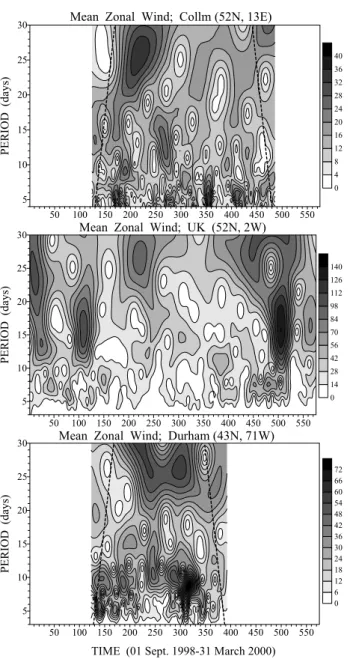
Fig. 2. Wavelet spectra of the zonal winds measured in Collm,
Ger-many (upper plot), in UK (middle) and in Durham, USA (bottom) in the period range 3–30 days.
oscillations present in the geomagnetic activity. Some strong events in the solar and geomagnetic records, however (e.g. days ∼ 150–170), are not reflected in the hmF2.
3.1 27-Day oscillations in spring 1999
As the 27-day oscillation, evident in the hmF2 around day number 250, is absent in the solar and geomagnetic activ-ity we investigated the neutral wind measured by the meteor radar at Durham. According to Luo et al. (2001) these os-cillations are stronger in the zonal component of the neutral wind. Figure 2 shows the wavelet transform of the mean zonal wind at Durham (bottom plot). Because of equip-ment problems the neutral wind measureequip-ments at Durham are available only in the interval 1 January – 30 September 1999.
150 180 210 240 270 300
NUMBER DAYS (started 01 Sept. 1998)
-8 -6 -4 -2 0 2 4 6 8 FI LT ERED DAT A (m /s )
27-Day Oscillation in Zonal Mean Wind Collm
Durham
UK
Fig. 3. The band-pass filtered zonal mean winds measured in Durham (thick solid line), Collm (thin solid line) and UK (dashed line). The filter is centred at period of 27 days.
This interval, however, includes the entire 27-day event that we investigate. There is very strong ∼ 27-day oscillation in the zonal wind simultaneously present with that in the iono-sphere. Even both maxima of the 27-day event around days 250 and 300 are evident in the plots of hmF2 and the zonal wind at Durham. Figure 2 (bottom plot) also displays wind oscillations at periods below ∼ 10–12 days that are not re-flected in hmF2. (These periods are of non-solar origin ac-cording to Fig. 1, because F10.7 does not display any oscil-lation at periods below 12 days.) However, dynamic forcing of the thermosphere-ionosphere system from below is possi-ble only if there is a global-scale oscillation observed in the MLT region. To determine whether the 27-day oscillation, or those with periods below 10–12 days, observed in the zonal wind at Durham are global-scale events, we have to use some additional neutral wind data. Accordingly, hourly data from the meteor radar at UK (52◦N, 2◦W) and daily data from the
LF drift measurements at Collm (52◦N, 13◦E) were used. The wavelet spectra of the neutral zonal wind at these ad-ditional stations are also shown in Fig. 2, as the upper plot represents the result for Collm and the middle plot - for UK. It is evident that the 27-day oscillation is a global-scale event, while the oscillations with periods below 10–12 days are ob-served mainly in Durham. (The 7–8-day oscillation around day 190 is only observed over Durham and Collm, but not over UK, so we will not investigate it in detail.) The 27-day oscillation observed over Europe however, has shorter dura-tion (only between day numbers 170 and 300) than that over North America. In the latter case there is the second ampli-tude maximum around day number 300 similar to the 27-day oscillation present in the hmF2 over Millstone Hill. To obtain some information about the real amplitudes of the 27-day os-cillation present in the zonal wind measured in these three stations we applied the band-pass filter centred at a period of 27 days and the results are shown in Fig. 3. The
global-D. Pancheva et al.: Variability in the maximum height of the ionospheric F2-layer 1811 50 100 150 200 250 300 350 400 450 500 550 5 10 15 20 25 30 PE R IO D (d ay s)
Crosswavelet Transform (Zonal Wind and hmF2)
0 1800 3600 5400 7200 9000 10800 12600 14400 16200 18000 19800 21600 23400 25200 0 50 100 150 200 250 300 350 400 450 500 550
TIME (01 Sept. 1998-31 March 2000) -3 -2 -1 0 1 2 3 PHAS E D IFFE RE NCE ( ra d)
Phase Difference between 27-day Oscillations in Mean Zonal Wind (Durham) and hmF2 (Millstone Hill)
Mean Phase Difference = 5-6 days
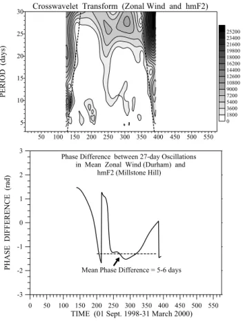
Fig. 4. Cross wavelet transform between the zonal mean wind at
Durham and hmF2 in Millstone Hill. The upper plot shows the power spectrum of the simultaneously existing oscillations in both time series, while the bottom plot indicates the phase difference between the 27-day oscillations observed in spring/early summer 1999.
scale character of this oscillation is clearly evident. Its am-plitude is about 8 m/s. Likewise, there is a hint of some west-ward direction of propagation. Using the least squares best fit method applied to the whole interval shown in Fig. 3 (be-tween day number 150 and 300) the calculated zonal wave number is 0.56. When this best fit method is applied only to the interval between day number 180 and 280, where three cycles are very well outlined, the result is 0.81, very close to 1. Therefore, we can accept that the global-scale 27-day oscillation in the zonal wind of the MLT region has west-ward direction of propagation with zonal wave number 1. To demonstrate the simultaneous presence of the 27-day oscil-lations in the neutral wind at Durham and in the ionospheric hmF2 parameter we performed the cross-wavelet transform between both time series. The obtained result is shown in Fig. 4. The upper plot shows the power spectrum where two clear maxima around 27 days are evident between days 230 and 340 and that indicate the simultaneous presence of these oscillations in the neutral MLT zonal wind at Durham and in the maximum height of the ionosphere F2-layer at Millstone Hill. The lower plot shows the phase difference between the above mention oscillations. The time delay between the
os-50 100 150 200 250 300 350 400 450 500 550 5 10 15 20 25 30 PER IOD (d ay s)
Crosswavelet Transform (ap-Index and hmF2)
0 3800 7600 11400 15200 19000 22800 26600 30400 34200 38000 0 50 100 150 200 250 300 350 400 450 500 550
TIME (01 Sept. 1998-31 March 2000) -3 -2 -1 0 1 2 3 PH ASE DIFF EREN CE (r ad)
Mean Phase Difference 0.8 - 1 day
Phase Difference between 27-Day Oscillations in ap-index and hmF2 (Millstone Hill)
Mean Phase Difference 6 - 7 days
Fig. 5. The same as Fig. 5, but between the geomagnetic Ap-index
and hmF2.
cillation in the ionosphere and the one in the zonal MLT wind is 5–6 days. This demonstrates that the 27-day oscillation is first evident in the zonal wind and the response of the iono-sphere follows 5–6 days later. The upper plot of Fig. 4 shows also a maximum between 6–8 days around days 190–200. It could be a result from the simultaneous presence of the 7– 8-day oscillation evident in the zonal wind at Durham (and Collm, but not at UK) and in the hmF2 at Millstone Hill.
To determine the relationship between the oscillations in the geomagnetic activity and those in the ionosphere hmF2 parameter we applied the cross-wavelet transform to the re-spective time series. The result is shown in Fig. 5. The upper plot shows three events simultaneously observed in the Ap-index and in the hmF2. These are a ∼ 23-day
wave around day number 70, and two 27-day oscillations around day numbers 330 and 430. The phase difference in the first and the third event is about 0.8–1 day. This means that if the geomagnetic activity is a reason for these oscil-lations, the response time of the ionosphere is less than one day, which is frequently observed (Pr¨olss, 1995). The empir-ical model recently created by Kutiev and Mukhtarov (2001), that describes the variations of midlatitude F-region ionisa-tion induced by geomagnetic activity, shows that the average response of the ionosphere to geomagnetic forcing is delayed with a time constant of about 18 h. Therefore, the observed 23- and 27-day oscillations in the ionospheric hmF2
param-1812 D. Pancheva et al.: Variability in the maximum height of the ionospheric F2-layer 50 100 150 200 250 300 350 400 450 500 550 5 10 15 20 25 30 PER IOD (da ys) Crosswavelet Transform (F10.7 - hmF2) 0 6000 12000 18000 24000 30000 36000 42000 48000 54000 60000 0 50 100 150 200 250 300 350 400 450 500 550
TIME (01 Sept. 1998-31 March 2000) -3 -2 -1 0 1 2 3 PHAS E D IFFE RE NCE (r ad )
Phase Difference between 27-Day Oscillations in F10.7 and hmF2 (Millstone Hill)
Mean Phase Difference 25-26 days
Fig. 6. The same as Fig. 5, but between the solar radio flux F10.7
and hmF2.
eter are most probably generated by the geomagnetic activ-ity. However, a problem arises from the second 27-day event (around day number 330), where the phase difference is more than 6–7 days. Usually the geomagnetic response is rather fast, not after 6 or more days. Consequently, this 27-day os-cillation in the ionosphere is most probably not related to the geomagnetic activity.
To determine the relationship between the oscillations in the solar activity and those in the ionospheric hmF2 param-eter we apply the cross-wavelet transform to the respective time series. The result is shown in Fig. 6. There is only a slight maximum with period 27–28 days around day number 320–330. However, the phase difference is positive and it means that the 27-day oscillation in the hmF2 appears more than 2 days ahead of that in the solar radio flux F10.7. Alter-natively, it can mean that the 27-day oscillation in the iono-sphere is delayed more than 25 days with respect to that in the F10.7. Such a long delay between both oscillations is impossible, so the solar radio flux F10.7 probably does not generate this oscillation in the ionosphere.
To demonstrate more clearly the relationship between the 27-day oscillations observed in the hmF2 from one side and those in the zonal wind at Durham, the geomagnetic Ap
-index and the solar radio flux F10.7 from the other side dur-ing sprdur-ing/summer 1999, we investigate the filtered data of the above mentioned parameters. The comparison between the 27-day filtered zonal wind at Durham (dashed line) and
140 160 180 200 220 240 260 280 300 320 340 360 380 -18 -15 -12 -9 -6 -3 0 3 6 9 12 15 FILT ERE D DATA (km, m/ s) Zonal wind (*2) Durham hmF2 140 160 180 200 220 240 260 280 300 320 340 360 380
DAY# (start 01 Sept. 1998)
-18 -15 -12 -9 -6 -3 0 3 6 9 12 15
FILTERED DATA (ap-index;
F10.7)
F10.7 (/4) ap-index
hmF2
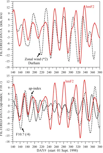
Fig. 7. The 27-day filtered zonal wind data at Durham (black dashed
line) and hmF2 at Millstone Hill (red line) observed in the interval between day numbers 140 and 380 (shown in the upper plot) and the 27-day filtered Ap-index (black solid line), F10.7 (black dashed
line) and hmF2 (red line) in the same time interval (lower plot).
the hmF2 (red line) is shown on the upper plot of Fig. 7. It is evident the simultaneous amplification of the 27-day oscil-lations in both parameters and their synchronous behaviour between days 220 and 340. The oscillation in the zonal wind generally leads that in the hmF2, especially after day number 280. In the bottom plot of the same figure there is a compar-ison between the 27-day filtered data for the Ap-index (solid
line) and F10.7 (dashed line) with that of the hmF2 (red line). It is evident that when the 27-day oscillation in the hmF2 is amplified (after day number 220) this oscillation is absent in the Ap-index and in the F10.7 also. So, the 27-day
os-cillation in the hmF2 evident between day number 220 and 300 is surely related to the 27-day variability in the zonal MLT region wind. After day number 280–300 however, the 27-day oscillation in the geomagnetic activity, as well as in the solar radio flux, starts to amplify. However, the 27-day oscillation in the zonal wind at Durham is still very strong until day number 340 after which it disappears. We point out that the 27-day oscillation in the hmF2 disappears also around day 340–350, nevertheless that the same oscillations
D. Pancheva et al.: Variability in the maximum height of the ionospheric F2-layer 1813 in the Ap-index and in the F10.7 continue to intensify. To be
more confident that the 27-day variability in the geomagnetic activity and in the solar radio flux evident after day number 300 are not responsible for the same oscillation in the hmF2, we perform cross correlation analysis between Ap-index and
hmF2 and between F10.7 and hmF2 for the time interval be-tween days 280 and 380 (see bottom plot of Fig. 7). The results of this analysis support the results from cross wavelet analysis, shown in Figs. 5 and 6. The 27-day oscillation in the Ap-index is 6 days ahead of that in the hmF2 and the same
oscillation in the F10.7 is 1.5 days behind that in the hmF2. In this study we take F10.7 as a proxy for the solar extreme ultraviolet (EUV) radiation that produces the F-layer ionisa-tion. According to Balan et al. (1993), F10.7 is a satisfac-tory indicator for long-term variations (year-to-year, possi-bly month-to-month) and probapossi-bly not so good at daily time scale, especially during high solar activity.
The cross wavelet and cross correlation analysis per-formed on the three pairs of data set shows that the 23-and 27-day oscillations in the ionosphere evident around day number 70 and 430 are probably generated by the geomag-netic activity, while the 27-day oscillations with maxima around day number 250 and 320 are probably generated by the similar global scale oscillations present in the zonal MLT region wind.
How can the PW oscillations originating in the middle atmosphere influence the thermosphere-ionosphere system? In Pancheva and Lysenko (1988) two possible mechanisms were discussed. One of them is valid mainly to the quasi-2-day oscillations and the other, the ionospheric wind dy-namo, involves the PW neutral wind motion to induce elec-tric fields. These elecelec-tric fields could modulate the height, or plasma density, of the ionospheric F-region. However, the numerical model created by Chen (1992) suggests that the wind magnitudes have to be on the order of a few tens of m/s in order to produce the electrodynamic effects inferred from observations. In our case, the observed amplitudes of 8 m/s are not strong enough, so, according to the numerical results, the global-scale 27-day oscillation in the zonal wind would probably not be able to generate electrodynamic ef-fects. But our observations support the suggestion that the variability of the MLT zonal wind most probably generates the 27-day oscillation in the ionosphere. Another mecha-nism, which in general contributes to the upward propaga-tion of planetary wave type oscillapropaga-tions into the F2-region, is modulation of upward propagating tides by planetary waves in the lower (lowest) thermosphere, as supported by exper-imental results (Lastovicka and Sauli, 1999), as well as by modelling (M¨uller-Wodarg, 1998).
3.2 16-Day oscillation in summer 1999
Figure 1 shows the 16–18-day oscillation in the ionosphere around day number 300, that is spread over summer months of 1999. There is no similar oscillation in the solar and/or in the geomagnetic activity. Figure 2 shows only slight sig-nature of 14–15-day wave during this time interval in the
0 91 182 273 364 455 546 240 260 280 300 320 340 DIURNAL AMPLITUDE S (k m) Diurnal Constant 0 91 182 273 364 455 546 0 20 40 60 80 100 DIURNAL AMPLITUDE S (k m)
Diurnal and Semidiurnal Amplitudes
0 91 182 273 364 455 546
TIME (01 Sept. 1998-31 March 2000)
0 2 4 6 8 10 12 DIURN A L PHASES (U T) 12-hour phase 24-hour phase
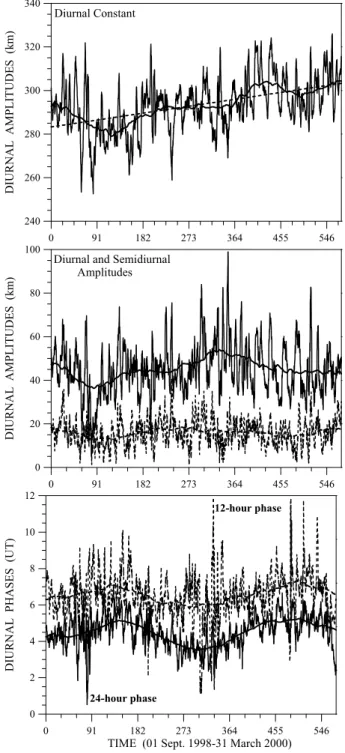
Fig. 8. Variability of the diurnal components of hmF2: the upper
plot describes the diurnal mean, the middle plot shows the ampli-tudes of 24-h (solid line) and 12-h (dashed line) harmonics and the bottom plot shows their phases. The thick solid or dashed lines in these plots describe the seasonal courses of these diurnal compo-nents obtained as the 3-month running mean.
neutral wind above Europe and about 12-day wave above Durham. During June–August 1999 a PSMOS (Planetary Scale Mesopause Observing System) MLT radar campaign was conducted and the basic aim of this campaign was to study the tidal variability. 23 MLT radars from Arctic to Antarctic latitudes participated in this campaign and they
1814 D. Pancheva et al.: Variability in the maximum height of the ionospheric F2-layer 50 100 150 200 250 300 350 400 450 500 550 5 10 15 20 25 30 PE R IO D (d ay s) C0 of hmF2 0 20 40 60 80 100 120 140 160 180 200 220 240 50 100 150 200 250 300 350 400 450 500 550 5 10 15 20 25 30 P E R IOD ( da ys ) A12 of hmF2 0 10 19 29 38 48 57 67 76 86 95 50 100 150 200 250 300 350 400 450 500 550
TIME (01 Sept. 1998-31 March 2000)
5 10 15 20 25 30 PE RIOD (d ay s) A24 of hmF2 0 20 40 60 80 100 120 140 160 180 200 220 50 100 150 200 250 300 350 400 450 500 550
TIME (01 Sept. 1998-31 March 2000)
5 10 15 20 25 30 PE RIO D (d ay s) Ph12 of hmF2 0 2 4 6 8 10 12 14 16 18 20
Fig. 9. The wavelet spectra of the diurnal mean (upper left plot), the amplitude of 24- (lower left plot) and 12-h (upper right plot) periodicities
of the hmF2 and the phase of the 12-h periodicity of the hmF2 (lower right plot) in the period range 3–30 days.
have provided knowledge of tidal winds, their amplitudes and phases, for comprehensive ranges of latitudes (equator to poles) with monthly (and higher) resolution. This cam-paign showed a weak 16-day wave mainly in the meridional component of the neutral wind, but very strong 16-day ulation of the semidiurnal tide. This strong 16-day tidal mod-ulation, with mean amplitude 7–8 m/s, is evident in both tidal components, suggesting a non-linear interaction with PW of that period to be responsible (Pancheva et al., 2002).
It is known that usually the PWs are not able to penetrate above 120 km, so their direct influence on the ionosphere variability is questionable. The numerical study of the 16-day wave (Forbes et al., 1995) showed also that this wave does not favour significant direct penetration into the dynamo region. The semidiurnal tide generated in the middle atmo-sphere and the tropoatmo-sphere by the absorption of solar radia-tion by ozone and water vapour, propagates vertically upward and participates in the dynamo generation of electric fields at higher levels. Forbes (1996) suggested that PWs could mod-ulate upward propagating tides and through them to mediate the PW signatures in the ionosphere.
If we assume that the observed 16-day oscillation in the ionospheric hmF2 parameter could be generated by the modulated MLT region semidiurnal tide, then probably the semidiurnal periodicity of the hmF2 has to be affected. In order to study the variability of the diurnal components of hmF2 we decompose it to the diurnal mean and 24-, 12- and 8-h harmonics. They are obtained on the basis of a 3-day
time segment that is moving through the time series each 3 h. Figure 8 shows the variations of the diurnal components, as the upper plot describes the diurnal mean, the middle plot shows the amplitudes of 24- (solid) and 12-h (dashed) har-monics and the lower plot shows their phases. The thick solid or dashed lines in these figures describe the seasonal courses of these components obtained as the 3-month run-ning mean. The diurnal components of the hmF2 have well expressed seasonal behaviour with clearly depicted short-term variability. Figure 9 shows the wavelet transform of the diurnal mean (left upper plot) and the amplitudes of 24- (left bottom) and 12-h harmonics (right upper). It is evident that around day number 300, when the hmF2 indicates 16-day os-cillation (Fig. 1), only the amplitude of the 12-hour harmonic demonstrates similar disturbance (it is shown by arrow). Fig-ure 9 also shows the wavelet transform of the phase of the 12-h harmonic (right bottom plot) and there a strong, visible 16-day oscillation (shown by an arrow). This result probably indicates, that if the modulated semidiurnal tide mediates the PW signature in the ionosphere, this PW oscillation has to be best expressed in the 12-h periodicity of the ionosphere.
In addition to the strong 16-day peak in the wavelet spec-trum of the amplitude of the 12-h hmF2 harmonic shown in the Fig. 10 (middle plot), there are also: (i) a 19–20-day peak around day number 150, (ii) a 24-day peak around day num-ber 230, and (iii) an 11-day peak around day numnum-ber 500. The wavelet spectrum of the phase of the 12-h harmonic (Fig. 10, bottom plot) indicates some additional variability
D. Pancheva et al.: Variability in the maximum height of the ionospheric F2-layer 1815
0 50 100 150 200 250 300 350 400 450 500 550
TIME (01 Sept. 1998-31 March 2000)
0 4 8 12 16 20 A M PL IT U D E (km)
Amplitude of Quasi-2-Day Wave in hmF2
0 50 100 150 200 250 300 350 400 450 500 550
TIME (01 Sept. 1998-31 March 2000)
0 50 100 150 200 250 3-H OURLY A P -INDEX ( nT )
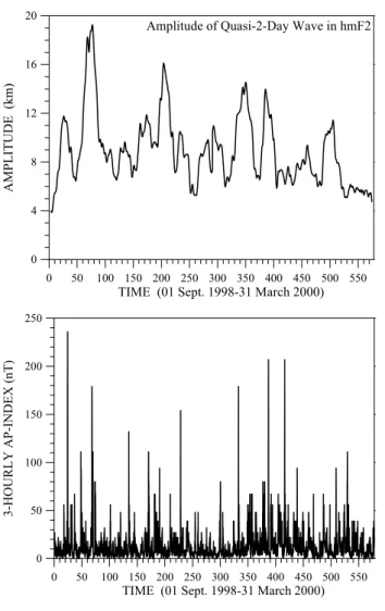
Fig. 10. The temporal variation of the instantaneous amplitudes
of the QTD oscillations in the hmF2 (upper plot), obtained by the complex demodulation method, and the 3-hourly geomagnetic Ap
-index shown on the bottom plot.
as: (i) a 15-day oscillation around day number 150 (but not 19–20 days as in the amplitude), (ii) there is no oscillation similar to the 24-day peak in the amplitude of the 12-h hmF2 harmonic around day number 230, and (iii) an 11-day peak around day number 490–500. Therefore, the same oscillation observed simultaneously in the amplitude and in the phase of the 12-h hmF2 harmonic is only an 11-day feature centred around day number 500. Some variability at this time is evi-dent also in the wavelet spectrum of the hmF2, but the mean period is about 9–10 days. Unfortunately, we have no neutral wind measurements at Durham and Collm during this time interval, so we have no information about the global-scale semidiurnal tidal variability that could be responsible for the 11-day oscillation evident in the amplitude and in the phase of the 12-h hmF2 periodicity.
3.3 Quasi-2-Day oscillations during equinoxes
There have been several papers, which delineate quasi-2-day (QTD) oscillations in the ionosphere (Pancheva and Lysenko,
10 20 30 40 50 60 70 80 90 5 10 15 20 25 30 PERIOD (d ay s)
Wavelet Transform of 3-Hourly ap-Index
0 15 30 45 60 75 90 105 120 135 150 165 180 10 20 30 40 50 60 70 80 90 10 20 30 40 50 60 70 PE RIOD (h ours ) 0 15 30 45 60 75 90 105 120 135 150 165 180
Wavelet Transform of 3-Hourly ap-Index
10 20 30 40 50 60 70 80 90
TIME (01 Sept.-30 Nov. 1998)
10 20 30 40 50 60 70 PE RIO D (hou rs)
Wavelet Transform of difhmF2
0 13 26 39 52 65 78 91 104 117 130
Fig. 11. Wavelet transform of the geomagnetic Ap-index in the
period range 1.5–30 days (upper plot), the wavelet transform of the same parameter, but in the period range 8–72 h (middle) and wavelet transform of the difference between the hourly data and the ref-erence diurnal course of the hmF2 (residual of hmF2) in the pe-riod range 8–72 h (bottom) for the time interval 1 September – 30 November 1998.
1988; Pancheva et al., 1994; Apostolov et al., 1995; Altadill et al., 1997; Forbes and Zhang, 1997; Forbes et al., 1997). Some of these are statistical studies involving the spectral analysis of multiyear data sets from specific ionosonde sta-tions and the others represent “case studies” wherein it was attempted to relate the F-region observation with the QTD wind oscillations in the MLT region. However, there is a sig-nificant discrepancy between the zonal structures of the QTD oscillations in the MLT region (usually with zonal wave num-bers 3 and 4) and those observed in the ionosphere (mainly zonal wave number 1, or a stationary oscillation with
inde-1816 D. Pancheva et al.: Variability in the maximum height of the ionospheric F2-layer
21 22 23 24 25 26 27 28 29 30
DAY# (start 01 Sept. 1998)
-250 -200 -150 -100 -50 0 50 D-st Index (nT) (a) 65 66 67 68 69 70 71 72 73 74 75 76 77 78 79
DAY# (start 01 Sept. 1998)
-150 -100 -50 0 50 D-st In dex (nT ) (b)
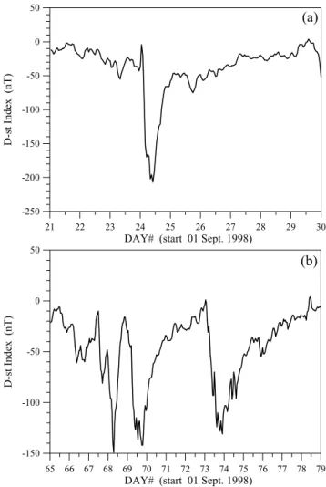
Fig. 12. Description of the geomagnetic storms in: (a) September
1998 and (b) in November 1998 by hourly Dst-index
terminable zonal wave number). It was shown that the QTD oscillations are quite regular disturbances of the summer F-region with typical amplitudes for foF2 in the range 0.4– 1.0 MHz and for hmF2 in the range of 8–16 km. Apostolov et al. (1995) and Altadill et al. (1997) showed that the average annual variation of the amplitudes of the QTD oscillation in the foF2 is modulated by the semiannual geomagnetic wave. This interesting result put a question why during the high ge-omagnetic activity (mostly during the equinoxes) we observe higher QTD oscillation activity in the ionosphere F-region.
We use this “case study” to investigate in detail the QTD oscillations in the hmF2, especially during the equinoxes, when the geomagnetic activity is high. As the QTD oscil-lations are short-period osciloscil-lations we will study them using the difference between the hourly data and the reference di-urnal course, composed by didi-urnal mean and 24-, 12- and 8-h harmonics, obtained by using sliding 3-day time seg-ments. To evaluate the temporal variation of the amplitudes of the QTD oscillations, the method of complex demodula-tion (Bloomfield, 1976) was applied. An effective band-pass filter was used with limits from 40 to 58 h for the 48-h
de-5 10 15 20 25 30 35 40 45 50 55 60 65 70 PERIOD (hours) 0 1 2 3 4 5 6 7 8 9 AM PL IT UDE SP ECTRUM 95%
Amplitude Spectrum of ap-index (01 Sept.-30 Nov. 1998) 5 10 15 20 25 30 35 40 45 50 55 60 65 70 PERIOD (hours) 0 1 2 3 4 5 6 7 8 AMPLITUDE S PECTRUM (km) 95%
Amplitude Spectrum of difhmF2 (01 Sept.-30 Nov. 1998)
Fig. 13. Amplitude spectra of the geomagnetic Ap-index (upper
plot) and of the residual of hmF2 (bottom) in the period range 4– 70 h obtained by the correloperiodogram analysis. The 95% confi-dence level is shown by dashed line.
modulation period. Figure 10 shows the temporal variation of the instantaneous amplitudes of the QTD oscillations in the hmF2 (upper plot) and the 3-hourly Ap-index in the lower
plot. There is positive relation between the high geomagnetic activity and the increase of the amplitudes of the QTD oscil-lations, especially well evident in the fall of 1998 and spring of 1999. As the strongest QTD oscillations in hmF2 are ob-served in the fall of 1998 we will study this seasonal interval in detail.
Figure 11 shows the wavelet transform of the 3-hourly
Ap-index in the period interval 1.5–30 days (upper plot), the
wavelet transform of the same parameter, but in the period range 8–72 h (middle plot) and the wavelet transform of the difference between the hourly data and the reference diur-nal course of hmF2 also in the period range 8–72 h (lower plot) for the time interval 1 September – 30 November 1998. The geomagnetic disturbances are clearly depicted in the up-per and middle plots and they are centred at day number 25 and 69. The description of these geomagnetic disturbances
D. Pancheva et al.: Variability in the maximum height of the ionospheric F2-layer 1817 through the hourly Dst-index is shown in Fig. 12. Enhanced
QTD oscillations at the days of the main phase of the storms and a few days later are evident in the ionosphere (lower plot of Fig. 11). The QTD oscillations related to the first geo-magnetic disturbance have mean periods ∼ 40–42 h and they are generated at the recovery phase of the geomagnetic dis-turbance. At the same time the main peak in the Ap-index
is ∼ 50 h and it is evident during the main phase of the stud-ied disturbances. The QTD oscillations related to the sec-ond geomagnetic disturbance are composed of a burst with mean period 42 h that coincides with the main phase of the storm and a second burst, with mean period 52–53 h, that is generated at the beginning of recovery phase after the third peak in the Dst-index (Fig. 12). Figure 13 shows the main
spectral peaks that are present in the geomagnetic Ap-index
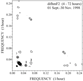
and in the analysed ionospheric data for the investigated 3-month time interval. There are two interesting features: (i) the main peaks in the ionosphere have periods 42 and 52.5 h and the same peak of 42 h is evident in the geomagnetic ac-tivity also. This suggests that the 42-h QTD oscillation evi-dent in the ionosphere during the main phase of the second geomagnetic storm (at day number 69 of the lower plot of Fig. 12) is probably generated directly by the similar oscilla-tion in the geomagnetic activity; (ii) in addioscilla-tion to the QTD peaks in the ionospheric data, there are also significant peaks, well above the 95% confidence level, with periods 11, 15 and 21 h (after the 24-, 12- and 8-h diurnal harmonics are removed). Why are these pseudo diurnal harmonics signifi-cantly strong during the geomagnetic storm? Fuller-Rowell et al. (1996) and Fuller-Rowell et al. (2000) offered a sce-nario (Similar to that already suggested by Pr¨olls, 1995) of the global response of the thermosphere-ionosphere system to magnetospheric energy input. This scenario is formulated around the temporal and spatial progress of the “composi-tion bulge”, as they called this region, where the gas mean molecular mass number is highest. Namely this composi-tion bulge, driven by the changed prevailing winds and in-situ generated tides (M¨uller-Wodarg et al., 2001) and its own temporal evolution, disturbs the usual diurnal behaviour of the ionosphere. Therefore, the strong pseudo diurnal peri-odicities evident in the amplitude spectrum of the residual of hmF2 during high geomagnetic activity are probably re-lated to the influence of this composition bulge. Figure 14 shows the bispectrum estimate calculated from the residual of hmF2. The non-zero points, marked as 1 and 2, represent the triplets (52.5, 21, 15) hours and (41.3, 15, 11) hours, re-spectively. However, Clark and Bergin (1997) pointed out, that the initial two mixing components could be any two of the three frequencies. Therefore, as strong pseudo diurnal periodicities are generated during high geomagnetic activity (Fig. 13), we may assume that 21- and 15-h frequencies in-teract to generate the QTD oscillation with period 52.5-h and that 15- and 11-h frequencies interact to generate the 41.3-h oscillation. T41.3-hese interactions between t41.3-he pseudo diurnal harmonics take place in the recovery phase of the geomag-netic storms, as is shown in the bottom plot of Fig. 11.
0.00 0.04 0.08 0.12 0.16 0.20 0.24 FREQUENCY (1/hour) 0.04 0.08 0.12 0.16 0.20 0.24 FREQU E NCY ( 1/h ou r) difhmF2 (4 - 72 hours) 01 Sept.-30 Nov. 1998 1 2
Fig. 14. The contour plot of the magnitude square bispectrum
cal-culated from the residual of the hmF2 data in the period interval 4–72 h.
4 Conclusions
The purpose of the present ‘case study’ is to investigate the variability in the maximum height of the ionospheric F2-layer, hmF2, with periods of planetary waves (2–30 days), and to make an attempt to determine their origin. The hourly data of the hmF2 above Millstone Hill (42.6◦N, 71.5◦W)
during 1 September 1998 - 31 March 2000 were analysed to study in detail three types of disturbances: the long-term 27-and 16-day oscillations 27-and the short-term quasi-2-day oscil-lations. The following main results were obtained:
– There were three different 27-day events observed in the hmF2: during autumn of 1998 and 1999 and during spring/early summer of 1999. Most probably the 27-day oscillation observed in the hmF2 above Millstone Hill in spring/early summer of 1999 is generated by the global-scale 27-day wave present in the zonal MLT neu-tral wind. The time delay between the 27-day oscilla-tion in the zonal wind and that in the hmF2 is found to be 5–6 days. The 27-day oscillations observed in au-tumn are generated by the geomagnetic activity. In this case the time delay between the 27-day oscillation in the geomagnetic activity and that in the hmF2 is 0.8–1 day. – The 16-day oscillation in the hmF2 observed during summer 1999 is probably generated by the global scale 16-day modulation of the semidiurnal tide observed in the MLT region during PSMOS campaign in June– August. When the modulated semidiurnal tide medi-ates the planetary wave signature in the ionosphere, this planetary wave oscillation has to be best expressed in
1818 D. Pancheva et al.: Variability in the maximum height of the ionospheric F2-layer the amplitude and in the phase of the 12-h periodicity
of the ionosphere.
– The quasi-2-day activity in the hmF2 increases during geomagnetic disturbances. The strong pseudo diurnal periodicities generated during the geomagnetic storms can interact between each other and produce the quasi-2-day oscillations in the ionosphere. This mechanism could explain why the average annual variation of the amplitudes of the QTD oscillation in the foF2 is modu-lated by the semiannual geomagnetic wave (Apostolov et al., 1995; Altadill et al., 1997). However, the ob-served QTD oscillation in the ionospheric F-region dur-ing summer is generated mainly by the quasi-2-day wave in the neutral wind of the MLT region.
Acknowledgements. Topical Editor M. Lester thanks D. Altadill and another referee for their help in evaluating this paper.
References
Altadill, D., Apostolov, E. M., and Alberca, L. F.: Some seasonal hemispheric similarities in foF2 quasi-2-day oscillations, J. Geo-phys. Res., 102, 9737–9739, 1997.
Apostolov, E. M., Altadill, D., and Alberca, L. F.: Characteristics of quasi-2-day oscillations in the foF2 at northern middle latitudes, J. Geophys. Res., 100, 12 163–12 171, 1995.
Apostolov, E. M., Altadill, D., and Hanbaba, R.: Spectral energy contributions of quasi-periodical oscillations (2–35 days) to the variability of foF2, Ann. Geophysicae, 16, 168–175, 1998. Balan, N., Bailey, G. J., and Jayachandran, B.: Ionospheric
evi-dence for a nonlinear relationship between the solar EUV and 10.7 cm fluxes during an intense solar cycle, Planet. Space Sci., 41, 141–145, 1993.
Beard, G. A., Mitchell, N. J., Williams, P. J. S., and Kunitake, M.: Non-linear interactions between tides and planetary waves result-ing in periodic tidal variability, J. Atmos. Sol.-Terr. Phys., 61, 363–376, 1999.
Bloomfield, P.: Fourier Analysis of Time Series: An Introduction, John Wiley, New York, 1976.
Chen, P. R.: Two-day oscillation of the equatorial ionisation anomaly, J. Geophys. Res., 99, 6343–6357, 1992.
Clark, R. R. and Bergin, J. S.: Bispectral analysis of mesosphere wind, J. Atmos. Sol.-Terr. Phys., 59, 629–639, 1997.
Forbes, J. M., Hagan, M.E., Miyahara, S., Vial, F., Manson, A. H., Meek, C. E., and Portnyagin, Yu.: Quasi-16-day oscillation in the mesosphere and lower thermosphere, J. Geophys. Res., 100, 9149–9164, 1995.
Forbes, J. M.: Planetary waves in the thermosphere-ionosphere sys-tem, J. Geomag. Geoelec., 48, 91–98, 1996.
Forbes, J. M. and Zhang, X.: Quasi 2-day oscillation of the iono-sphere: A statistical study, J. Atmos. Sol.-Terr. Phys., 59, 1025– 1034, 1997.
Forbes, J. M., Guffee, R., Zhang, X., Fritts, D., Riggin, D., Manson, A., Meek, C., and Vincent, R. A.: Quasi-2-day oscillation of the ionosphere during summer 1992, J. Geophys. Res., 102, 7301– 7305, 1997.
Forbes, J. M., Palo, S. E., and Zhang, X.: Variability of the iono-sphere, J. Atmos. Sol.-Terr. Phys., 62, 685–693, 2000.
Foster, J. C., Holt, J. M., Musgrove, R. G., and Evans, D. S.: Iono-spheric convection associated with discrete levels of particle pre-cipitation, Geophys. Res. Lett., 13, 656–659, 1986.
Fuller-Rowell, T. J. and Evans, D. S.: Height-integrated Peder-sen and Hall conductivity patterns inferred from TIROS-NOAA satellite data, J. Geophys. Res., 92, 7606–7618, 1987.
Fuller-Rowell, T. J., Codrescu, M. V., Moffett, R. J., and Quegan, S.: Response of the thermosphere and ionosphere to geomagnetic storms, J. Geophys. Res., 99, 3893–3914, 1994.
Fuller-Rowell, T. J., Condrescu, M. V., Rishbeth, H., Moffett, R. J., and Quegan, S.: On the seasonal response of the thermosphere and ionosphere to geomagnetic storms, J. Geophys. Res., 101, 2343–2353, 1996.
Fuller-Rowell, T. J., Codrescu, M. V., and Wilkinson, M.: Quanti-tative modelling of the ionospheric response to geomagnetic ac-tivity, Ann. Geophysicae., 18, 766–781, 2000.
Hagan, M. E., Forbes, J. M., and Vial, F.: On modelling migrating solar tides, Geophys. Res. Lett., 22, 893–896, 1995.
Hagan, M. E., Burrage, M. D., Forbes, J. F., J. Hackney, Randel, W. J., and Zhang, X.: GSWM-98: Results for migrating solar tides, J. Geophys. Res., 104, 6813–6828, 1999.
Hagan, M. E., Roble, R. G., and Hackney, J.: Migrating thermo-spheric tides, J. Geophys. Res., 106, 12 739–12 752, 2001. Kutiev, I. and Mukhtarov, P.: Modeling of midlatitude F-region
re-sponse to geomagnetic activity, J. Geophys. Res., 106, 15 501– 15 509, 2001.
Kopecky, M. and Kuklin, G.: About 11-year variation of the mean life duration of a group sun spots, Issled. Geomagn. Aeronom. Foz. Solntsa, 2, 167, 1971.
Lastovicka, J. and Sauli, P.: Are planetary wave type oscillations in the F2-region caused by planetary wave modulation of upward propagating tides? Adv. Space Res., 24, 1473–1476, 1999. Luo, Y., Manson, A. H., Meek, C. E., Igarashi, K., and Jacobi, Ch.:
Extra long period (20–40 day) oscillations in the mesosphere and lower thermosphere winds: Observations in Canada, Europe and Japan, and considerations of possible solar influences, J. Atmos. Sol.-Terr. Phys., 63, 835–852, 2001.
Miyahara, S. and Wu, D. H.: Effects of solar tides on the zonal mean circulation in the lower thermosphere: Solstice condition, J. Atmos. Terr. Phys., 51, 635–648, 1989.
M¨uller-Wodarg, I. F. C.: Propagation of planetary waves into the thermosphere and ionosphere - a modelling study, XXIII EGS, Nice, Book of Abstracts, p. C846, 1998.
M¨uller-Wodarg, I. F. C., Aylward, A. D., and Fuller-Rowell, T. J.: Tidal oscillations in the thermosphere: a theoretical investigation of their sources, J. Atmos. Sol.-Terr. Phys., 63, 899–914, 2001. Pancheva, D. and Lysenko, I.: Quasi-two-day fluctuations observed
in the summer F-region electron maximum, Bulg. Geophys. J., 14(2), 41–51, 1988.
Pancheva D., Schminder, R., and Lastovicka, J.: 27-day fluctuations in the ionospheric D-region, J. Atmos. Terr. Phys., 53, 1145– 1150, 1991.
Pancheva, D., Alberca, L., and de la Morena, B.: Simultaneous observation of the quasi-two-day wave variations in the lower and upper ionosphere over Europe, J. Atmos. Terr. Phys., 56, 43– 50, 1994.
Pancheva, D.: Evidence for non-linear coupling of planetary waves and tides in the lower thermosphere over Bulgaria, J. Atmos. Sol.-Terr. Phys., 62, 115–132, 2000.
Pancheva, D. and Mukhtarov, P.: Wavelet analysis on transient be-haviour of tidal amplitude fluctuations observed by meteor radar in the lower thermosphere over Bulgaria, Ann. Geophysicae., 18,
D. Pancheva et al.: Variability in the maximum height of the ionospheric F2-layer 1819 316–331, 2000.
D. Pancheva, Merzlyakov, E., Mitchell, N. J., Portnyagin, Yu., Man-son, A. H., Jacobi, Ch., Meek, C. E., Luo, Y., Clark, R. R., Hock-ing, W. K., MacDougall, J., Muller, H. G., K¨urschner, D., Jones, G. O. L., Vincent, R. A., Reid, I. M., Singer, W., Igarashi, K., Fraser, G. I., Fahrutdinova, A. N., Stepanov, A. M., Poole, L. M. G., Malinga, S. B., Kashcheyev, B. L., and Oleynikov, A. N.: Global scale tidal variability during the PSMOS campaign of June–August 1999 with periods of planetary waves, J. Atmos. Sol.-Terr. Phys., in press, 2002.
Pr¨olss, G. W.: Ionospheric F-region storms, in: Handbook for At-mospheric Electrodynamics, vol. 2, (Ed) Volland, H., CRC Press, Boca Raton, pp. 195–248, 1995.
Reinisch, B.: Modern Ionosonde, in: Modern Ionospheric Science, (Eds) Kohl, H., R¨uster, R., and Schlegel, K., EGS, Katlenburg-Lindau, Germany, pp. 440–458, 1996.
Rishbeth, H. and Mendillo, M.: Patterns of F2-layer variability, J. Atmos. Sol.-Terr. Phys., 63, 1661–1680, 2001.
Torrence, C. and Compo, G.: A practical guide to wavelet analysis, Bull. Amer. Meteor. Soc., 79, 61–78, 1998.