Adaptive communication in multi-robot systems using directionality of signal strength

Adaptive communication in multi-robot

systems using directionality of signal strength

The MIT Faculty has made this article openly available.

Please share

how this access benefits you. Your story matters.

Citation

Gil, S., S. Kumar, D. Katabi, and D. Rus. “Adaptive Communication in

Multi-Robot Systems Using Directionality of Signal Strength.” The

International Journal of Robotics Research 34, no. 7 (May 18, 2015):

946–968.

As Published

http://dx.doi.org/10.1177/0278364914567793

Publisher

Sage Publications

Version

Author's final manuscript

Citable link

http://hdl.handle.net/1721.1/100520

Terms of Use

Creative Commons Attribution-Noncommercial-Share Alike

Adaptive Communication in Multi-Robot Systems

Using Directionality of Signal Strength

Stephanie Gil, Swarun Kumar, Dina Katabi, Daniela Rus

Massachusetts Institute of Technology, MA.

{sgil,swarun,dk,rus}@mit.edu

Abstract— We consider the problem of satisfying commu-nication demands in a multi-agent system where several robots cooperate on a task and a fixed subset of the agents act as mobile routers. Our goal is to position the team of robotic routers to provide communication coverage to the remaining client robots. We allow for dynamic environments and variable client demands, thus necessitating an adaptive solution. We present an innovative method that calculates a mapping between a robot’s current position and the signal strength that it receives along each spatial direction, for its wireless links to every other robot. We show that this information can be used to design a simple positional controller that retains a quadratic structure, while adapting to wireless signals in real-world environments. Notably, our approach does not necessitate stochastic sampling along directions that are counter-productive to the overall coordination goal, nor does it require exact client positions, or a known map of the environment.

I. INTRODUCTION

There are many projects on today’s frontier that are pushing the capabilities of multi-agent systems. Swarm robotic systems perform many complex tasks through coordination, such as cooperative search of an environment, consensus, rendezvous, and formation control [Cortes et al., 2004; Jadbabaie et al., 2003; Olfati-Saber et al., 2007]. Google’s Project Loon, Face-book’s Connectivity Lab, and similar projects envision using a network of controllable routers to provide wireless communi-cation infrastructure in remote areas of the world. At their core, these systems rely on coordination between agents [Cortes et al., 2004; Moreau, 2004; Spanos and Murray, 2005; Tahbaz-Salehi and Jadbabaie, 2007], making reliable communication of primary importance. Beyond simply maintaining connec-tivity, reliable communication may mean supporting heteroge-neous and possibly time-varying communication rates amongst different pairs of agents. For example, some agents may need to use the network for transmitting video while others may simply wish to transmit status information.

We focus on problems where an auxiliary team of robot routers can be deployed to establish reliable wireless com-munication to a team of client agents who are performing an independent task. As depicted in Figure 1, we wish to control the positions of robot routers to establish communication links that are capable of supporting variable demanded rates to the client agents. The problem of providing wireless communi-cation coverage amongst multi-robot systems requires tight feedback between spatial positioning of the robots and sensing of the communication quality. The richer the information on signal quality, the more effective the control. A key realization makes this problem very challenging: Robotic tasks leverage mobility in Euclidean space and thus require knowledge of how position effects communication. However, the relationship of signal quality with spatial position is notoriously hard to

O b st ac le 50 Mb/s 12 Mb/s 30 Mb/s Legend Router Robot Client Agent

Fig. 1. Picture of a network of two robot routers satisfying the demands of

three clients in an environment with an occluding obstacle whose position is unknown.

predict due to complex interactions with the environment such as multipath, where the signal is reflected and/or attenuated by multiple objects in the environment before arriving at a receiver [Goldsmith, 2005; Lindhe et al., 2007; Malmirchegini and Mostofi, 2012]. Past literature employs two broad strate-gies to address this challenge. On the one hand, there is the Euclidean disk model which assumes that the signal quality of a link is a function of distance between the communi-cating vehicles. This model is deterministic and simple, and hence when incorporated in a robotic controller, yields simple positional optimizations for a wide range of collaborative tasks [Cortes et al., 2004; Jadbabaie et al., 2003; Olfati-Saber et al., 2007]. Unfortunately, the Euclidean model is too simplistic and fails to represent wireless signals in realistic environments [Malmirchegini and Mostofi, 2012]. On the other hand, there are stochastic sampling methods [Fink et al., 2012; Malmirchegini and Mostofi, 2012; Yan and Mostofi, 2013a] that measure the wireless signal strength in a robot’s vicinity to fit parameters for intricate probabilistic commu-nication models. While such methods are not oblivious to wireless channels, they require exploratory sampling [Lindh´e and Johansson, 2010] along directions that may be counter-productive to the overall coordination goal. Further, they often assume the knowledge of parameters based on the structure and material composition of the environment.

Our objective is to i) present a novel method to capture the spatial variation of wireless signals in the local environ-ment without sampling along counter-productive directions, or requiring information about the environment or the channel’s distributions and ii) derive a control formulation that maintains the structural (quadratic) simplicity allowed by the Euclidean disk model while accounting for wireless channel feedback.

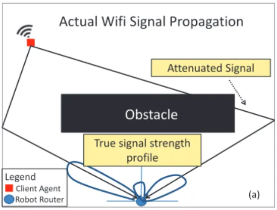
Actual Wifi Signal Propagation

True signal strength profile (a) Attenuated Signal Obstacle Legend Client Agent Robot Router

Fig. 2. Schematic drawing of a true signal strength profile in the local

environment of a robotic router. Large lobes indicate directions of high signal strength.

First, we introduce an innovative approach for mapping communication quality to robot placement. We calculate a mapping between a robot’s current position and the signal strength that it receives along each spatial direction, for every wireless link with other robots (see Figure 2). This is in contrast to existing methods [Fink et al., 2012; Yan and Mostofi, 2013a], which compute an aggregate signal power at each position but cannot distinguish the amount of signal power received from each spatial direction. Our approach combines the best attributes of both the Euclidean disk model and the stochastic sampling methods: Like the disk model, we can compute our mapping without knowledge of the environment and its obstacles, or a model of the channel’s distribution. Like the stochastic methods, our approach uses feedback from the actual wireless signals and hence can help multi-robot systems satisfy their desired communication demands in a real-world implementation. A naive approach to achieve this would be to mount directional antennas atop the routers; but these antennas are bulky and prohibitive for small agile platforms [Networks, 2014]. Instead, we present a novel algorithm based on Synthetic Aperture Radar (SAR) [Fitch, 1988], where a single omnidirectional antenna emulates a high-resolution directional antenna. This paper presents the first such algorithm for implementing SAR using off-the-shelf wireless cards in a non-radar setting, a challenging task since these devices are not intended for this purpose.

Second, we construct an optimization for positioning a team of robot routers to provide communication coverage over client vehicles using the directional information provided by our mapping. Being able to measure the profile of signal strength across spatial directions in real-time yields a much more capable controller. For example, the direction that im-proves signal strength the most is immediately attainable from these profiles (see Figure 2 for a schematic interpretation). Therefore as a direct consequence, the controller has access to the gradient of communication quality for each of its “links”, or neighbors to which it communicates. While in the favorable scenario, there is a single recommended direction of movement, in real-world implementations it is possible for there to be multiple such directions due to multipath or even noise that may be affecting the wireless link. This information is important for gauging the confidence with which the controller can improve signal quality by navigating the robot along any of the recommended directions. To this end, we present a method for computing a confidence metric

from the data and show that this metric can accurately and automatically identify the three scenarios of strong single-peak, multi-single-peak, or noisy peak in actual experimental data. Our control algorithm leverages the gradient directions and their associated confidences to automatically tune the speed of the robot, improving both stability and convergence time. Finally, our controller optimizes communication with multiple robots by choosing a direction of movement corresponding to a strong signal that strikes trade-offs between competing demands.

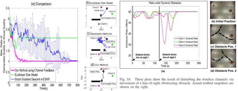
The result of a tight integration between our wireless signal quality mapping and positional controller yields algorithms for router placements that do not rely on environment-dependent parameters, obstacle maps, or even client positions. The overall solution presented is adaptive to variable communication qual-ity demands by the clients, as well as changes in the wireless channels due to natural fluctuations or a dynamic environment. We implement our method in a multi-robot testbed that has two robotic routers serving three robotic clients. We conduct our experiments in different indoor environments without providing the robotic controller the environment map or the clients’ positions. We observe the following: 1) Our system consistently positions the robotic routers to satisfy the robotic client demands, while adapting to changes in the environment and fluctuations in the wireless channels; 2) Compared to the disk model [Cortes et al., 2004; Jadbabaie et al., 2003] and the stochastic approach [Le Ny et al., 2012; Spall, 2000] under identical settings, our system converges to accurately satisfy the communication demands, unlike the disk model, while significantly out-performing the stochastic method in terms of empirical convergence rate (see Fig. 15 in Sec. VI-E). A. Contributions

We present a method to enable a robotic receiver to find the profile of signal strength across spatial directions for each sender of interest. To this end, we perform synthetic aperture radar (SAR) techniques using standard Wi-Fi packets exchanged between two independent nodes with single omni-directional antennas. We derive a quantitative metric, the confidence, that can accurately and automatically identify the presence of multipath or noise for each communication link. This provides valuable information to the controller in gauging the effectiveness of each recommended direction of movement in improving communication quality. We develop an optimization that leverages the directional signal profiles and their confidences, to position robotic routers to satisfy het-erogeneous (and possibly variable) communication demands of a network of robotic clients, while adapting to real-time en-vironmental changes. Finally, we provide aggregate empirical data to show that our method outperforms existing Euclidean disk or Stochastic sampling methods both in convergence

time (3.4× faster) and variability of performance (4× smaller

variance).

II. RELATEDWORK

Related work falls under two broad categories. A. Multi-Robot Coordination

Our work is related to past papers on multi-robot coordina-tion to achieve a collaborative task while supporting specific

communication demands [Fink et al., 2012; Le Ny et al., 2012; Malmirchegini and Mostofi, 2012; Yan and Mostofi, 2013a]. Past work on this topic fall under two classes of approaches. Euclidean Disk Model: The first class employs Euclidean disk assumptions where signal quality is assumed to be de-terministic and mapped perfectly to the Euclidean distance between the communication nodes. A Euclidean metric allows for quadratic cost for the edges of the network and enables a geometric treatment of an otherwise complex problem. In reality, signal strength suffers from large variations over small displacements [Goldsmith, 2005; Lindhe et al., 2007] that these models simply do not capture. Yet, the simplicity afforded by these models has led to significant contributions including i) multi-agent coordination for coverage and flock-ing [Martinez et al., 2007; Schuresko and Cortes, 2009], ii) assignment of routers to clients for attaining a prescribed level of connectivity [Feldman et al., 2013; Gil et al., 2012] or throughput [Craparo et al., 2011], and iii) connectivity maintenance based on graph theoretic approaches [De Gennaro and Jadbabaie, 2006; Michael et al., 2009].

Stochastic Sampling Methods: Recently, efforts have

fo-cused on giving the communication quality over each link in the network a more realistic treatment by sampling the signal strength and building closed-loop controllers using this feedback. Such stochastic sampling methods either supple-ment theoretical models for signal strength with a stochastic component based on the collected samples [Lindhe et al., 2007; Malmirchegini and Mostofi, 2012], or, use the collected samples to design stochastic gradient controllers [Le Ny et al., 2012; Twigg et al., 2013]. These papers have studied stochastic sampling patterns for i) acquiring sufficient signal strength (RSS) samples [Lindhe et al., 2007; Lindh´e and Johansson, 2010], ii) co-optimizing communication quality and other higher level tasks like motion planning or message routing [Fink et al., 2013; Yan and Mostofi, 2013b], iii) used router mobility to escape “deep fades” or null points where connectivity may be lost [Vieira et al., 2013] or to map out the signal strength and resulting connectivity regions of the environment [Twigg et al., 2013]. Unfortunately these works necessitate at least one of the following prohibitive requirements: i) motion of the routers along counter-productive paths to collect sufficient RSS samples, ii) assumptions of a known environment map, static surroundings, and known positions of communicating agents, or iii) previously acquired signal strength maps.

In comparison to these papers, we introduce a system that captures the magnitude of the signal arriving from different directions, as opposed to only its total magnitude at a particular position. This allows us to combine the best of both the disk model and stochastic sampling methods: Like the disk model, we do not require prior knowledge of the environment and its obstacles, or a model of channel’s distribution. Like the stochastic methods, our approach accurately captures actual signal characteristics and hence can help multi-robot systems satisfy their desired communication demands in real-world environments. Figure 3 provides an illustrative example of how our system out-performs the Euclidean disk model and stochastic sampling, particularly in the presence of obstacles.

B. Angle of Arrival Systems

Our method builds upon a rich body of literature in wireless networking that estimates actual angle-of-arrival of each of the reflected paths of a signal at a receiving device. Past work has employed two classes of hardware to estimate angle-of-arrival:

Antenna Arrays: Past literature has leveraged arrays of

antennas to estimate angle-of-arrival for localization [Joshi et al., 2013; Wang and Katabi, 2013; Xiong and Jamieson, 2013] and tracking [Pham and Sadler, 1997]. These use stationary multi-antenna receivers to locate the transmitter with sub-meter accuracy. Unfortunate for the robotics community, many of these techniques require bulky, specialized hardware such as customized software radios, and are thus difficult to place on small, agile, mobile platforms that are ubiquitous for robotics applications.

Synthetic Aperture Radar: Understanding how to attain

this directional information using a moving platform is the subject of Synthetic Aperture Radar (SAR) [Fitch, 1988]. SAR allows even a single-antenna mounted on a flying aircraft or satellite to emulate a multi-antenna array. Unfortunately, most SAR applications [Fitch, 1988; Wang et al., 2013; Wang and Katabi, 2013] are geared towards radar-type problems (eg. imaging, RFID applications) where signals are transmitted and processed by the same node. Therefore, they cannot be used to analyze the direction of arrival of the signal from a distinct transmitter (e.g. Wi-Fi devices).

For an adaptive communication network of small router robots, we need a light-weight, single-antenna system that can perform SAR using two-way transmissions (unlike radar) on off-the-shelf Wi-Fi devices. In this regard, we develop a system that builds upon synthetic aperture radar meant for robotic routers and clients equipped with standard Wi-Fi cards. C. Organization

Section III presents a formulation of the router placement problem for achieving communication coverage for clients with heterogeneous demands. The following sections describe each component of our solution to the problem:

• Section IV derives a new method for measuring rich

directional information from wireless channel feedback.

• Section V presents an algorithm for finding a

configura-tion of routers that balances the network, i.e. maximizes the signal quality of the weakest link for a fair network.

• In Section V-B we derive a confidence metric using

channel feedback, that captures the effects of multipath and noise.

Finally, Section VI experimentally evaluates our approach against the disk model and stochastic sampling methods.

III. PROBLEMSTATEMENT

We consider a mobile network with two classes of members, n robotic clients (or clients) whose positions are not controlled, and a team of k robotic routers whose mobility we control. Our goal is to position the robotic routers to provide adaptive wireless communication coverage to the clients, while allow-ing variable communication quality demands for all clients, and where exact client positions are unknown. For each

client j∈ [n] = {1, . . . , n}, we define demanded communication

quality qj> 0, and achieved communication qualityρi jto each

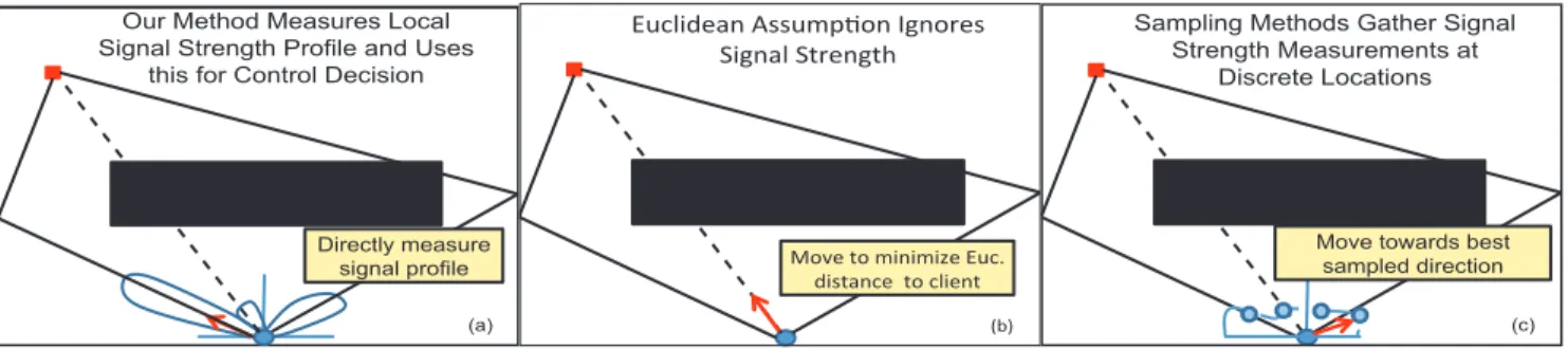
Our Method Measures Local Signal Strength Profile and Uses

this for Control Decision

(a) Directly measure signal profile !"#$%&'()*+,,"-./0)*12)03',* 4%2)($*453')256* 789* :0;'*50*-%)%-%<'*!"#=* &%,5()#'**50*#$%')5**

Sampling Methods Gather Signal Strength Measurements at

Discrete Locations

(c) Move towards best

sampled direction

Fig. 3. Compares our method against the Euclidean disk model and a stochastic sampling. The figures depict the actual router (blue) and client (red) separated by an obstacle (black). The black lines indicate the different paths of the signal. (a) Our method estimates the actual signal power arriving from different angular directions, much like a high-resolution directional antenna would. This provides a sharpened peak in the direction of maximum signal strength. (b) The Euclidean Disk model guides the router along the shortest Euclidean path, which is greatly attenuated by the obstacle. (c) Stochastic methods measure the signal strength by moving the router and sampling at various positions (blue circles). The signal strength does not vary significantly between locations due to the lack of spatial resolution, ie. at each sample location the signal strength is a combination of signals arriving from all angular directions. This leads to much less discernible peaks when contrasted with (a) (Note that the polar plot of signal power, shown here as dotted lines, have peaks in the same angular directions as our method though less sharp ). This method guides the router towards the direction of the best sample, which often may not be the actual direction of maximum signal strength, as shown.

Signal to Noise Ratio (ESNR) that has a direct mapping to

rate in Mb/s [Halperin et al., 2010].1 _{Additionally, let every}

client j be given an importanceαj> 0. We allow all quantities

in this section (ie. qj,ρi j,αj) to be time dependent though we

omit this dependency henceforth for simplicity.

We define the notion of service discrepancy for each pair

of robots(i, j) to be the difference between the demanded and

achieved communication quality scaled by the importance of the client.

wi j= max(αj(qj−ρi j)/qj, 0) (1)

Physically, this is the fraction of the client’s communication

demand that remains to be satisfied, scaled by αj. Denote by

ci∈ Rd the position of the ith robot router and by pj∈ Rd

the position of the jth client and Ct = {c1,t, . . . , ck,t} is the

set of all router positions at time t. In this paper we give

explicit treatment to the case for d= 2 although all concepts

are extensible to d= 3.

A. Problem Formulation

Given a cost g in terms of signal quality, communication demands, and agent positions, we wish to position each robotic router to minimize the largest discrepancy of service between routers and clients. However, the true form of this function g has an intricate dependence on the position of the client, router, and the environment. Thus an inherent challenge to solving this problem is approximating the influence of spatial positioning on communication quality that generalizes across

environments. Our goal is to 1) find fi j :[−₂π,π₂] → R (a

relation capturing directional information about the signal

quality between i and j), and an approximation ˜g of g, which

is a cost, characterizing the anticipated communication quality

for the router-client pair(i, j) at a proposed router position ci,

and 2) use this cost to optimize router positions to minimize the service discrepancy to each client. Formally,

Problem 1: Find i) a mapping fi j:[−₂π,π₂] → R that maps

spatial direction to wireless signal strength directly from

1_{ESNR is a continuous signal quality measure that has a one-to-one}

mapping to the maximum data rate supported by a link [Halperin et al., 2010]. We work with ESNR values rather than rates since the latter are discretized (non-continuous).

channel measurements, and ii) a cost ˜

g(ci,Ct, wi j, fi j) > 0 (2)

that is independent of the environment and satisfies the fol-lowing properties:

Property 1: All link costs ˜g are quadratic

Property 2: Minimization of a link cost ˜g over ci directly

relates to increasing signal quality for client j and optimization

over all link costs ˜g allows trade-offs between clients with

competing demands

Property 3: The link costs ˜g are independent of client

positions pj

Given a known number k of routers, client demands qd, and

the mapping fi j for all links in the network, position routers

to minimize the worst-case link. Specifically, we aim to find a position for the routers that minimizes the maximum service discrepancy by solving for C in the following problem:

Ct+1= argmin

ci∈C

{max

j mini g˜(ci,Ct, wi j, fi j)} (3)

Intuitively, the solution to this optimization problem favors a “fair” network. Specifically, the solution aims to minimize the “worst service discrepancy” among clients in the network, at any point in time. The worst service discrepancy is given mathematically by the bracketed expression in Equation (3) and can be understood intuitively as follows: 1) The service discrepancy of a router-client link captures the difference between the measured quality of the link and the client’s demanded communication quality (see Equation (1)). 2) Each client is served by a router that offers the minimum service discrepancy to it, at any given time (the innermost min over i in Equation (3) above). 3) The worst service discrepancy, is the maximum service discrepancy among all clients to their chosen routers in the network (the inner max over j in Equation (3)). Notice that the client with the worst service discrepancy may change at any point in time, depending on the configuration of the routers. The optimal configuration of the routers (given by the outer arg min term), is therefore the configuration that best satisfies communication demands across the entire network.

B. Problem Scope

We specify that our aim in this paper is to position mobile routers to establish a communication network whose links have high enough ESNR to support given client

communi-cation demands, qd. In other words, we are interested in

providing the infrastructure to support the requested quality of communication. This is in contrast to solving for routing protocols that would optimize the communication traffic over the infrastructure to ensure successful message passing from a sending node to a receiving node. While this is another common metric of connectivity, it is often times treated as a layer on top of an existing communication infrastructure and is an out-of-scope problem with a vast body of dedicated literature (See [Fink et al., 2010] for an example of routing in robotic networks). Finally, we assume throughout that router-router links are high capacity and that router-router-client links are the limiting factor that must be optimized.

We dedicate the next sections of this paper to 1) Developing

a method that computes fi j as the profile of signal qualities

along each directionθ for each link(i, j) found directly from

channel measurements; and 2) Developing an optimization framework that utilizes this directional information to handle trade-offs between competing client demands, and position all routers to jointly minimize the maximum service discrepancy across links in the network.

IV. DIRECTIONALPOWERPROFILE OF AWIRELESSLINK

In this section, we develop the first component of the solution of Problem 1; namely, we derive a method to calculate

f(θ), the mapping to capture the signal strength from a robotic

client to its router along each directionθ, where this mapping

can be updated often, roughly once every 6cm of motion.2

Before we explain how we compute f(θ), we describe this

function to help understand what it captures. Assume we have a robotic client and router, where the router moves along

some trajectory. We will define the directionθ relative to the

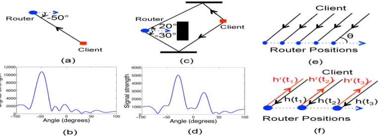
tangent to the router’s trajectory at each point. Consider the scenario in Fig.4(a), where the robotic client is in line-of-sight

at−50◦ _{relative to the robotic router, which is moving along}

the horizontal axis. In this case, one would expect f(θ) to

have a single dominant peak at −50◦_{, as shown in Fig.4(b).}

Now consider the more complex scenario in Fig.4(c), where the environment has some obstacles and one of these obstacles obstructs the line-of-sight path between the router and its

client. In this case, f(θ) would show two dominant peaks

at 20◦ and −30◦ that correspond to the two reflected paths

from surrounding obstacles, as shown in Fig.4(d).

Advantage over Sampling Methods: One may estimate

f(θ) by sampling the signal power similar to stochastic

techniques [Le Ny et al., 2012; Spall, 2000; Yan and Mostofi, 2013a]. In this case, one has to move the router along each direction, compute the power in all these new positions relative

to the first, and draw the profile f(θ). Unfortunately, this

approach leads to much wasted exploration. This is because the signal power does not change reliably when the robot moves. For example, if the robot moves for 5 or 10 centimeters, it is very likely that the resulting change in the signal power is below the variability in noise. Hence, measurements of

2_{For simplicity, we denote f}

i j(θ) as f (θ) as we consider only the single

link between robotic router i and client j for the rest of this section.

power over short distances are likely to be marred by noise or phenomena that affect the signal strength locally such as deep fades [Tse and Viswanath, 2005] (due to reflections of the signal at the receiver interfering constructively or destructively). To obtain reliable measurements of changes in the signal power, the robot has to move significantly along potentially counter-productive paths.

To address this limitation, our approach relies on the channel phase as opposed to the power. Specifically, at any position the wireless channel can be expressed as a complex number

h(t) [Rahul et al., 2012]. The magnitude of this complex

channel captures the signal power (more accurately, its square-root). The phase of the channel has traditionally been ignored by robotic systems. However, the phase changes rapidly with motion. For Wi-Fi signals at a frequency of 5 GHz, the phase

of the channel rotates byπ every 3 cm. This far exceeds any

rotation due to noise variability. Thus, by measuring channels as complex numbers and tracking changes in its phase as the robot moves, we reliably estimate signal variation without much exploration. In the next section, we explain how to use a technique called synthetic aperture radar (SAR) to extract the received signal strength along each direction from changes in channel phase. Note that SAR does not need exploration in all directions; the robot can move along its path without extra exploration or sampling. SAR uses the resulting variations in

channel phase over distances of a few centimeters to find f(θ).

A. Synthetic Aperture Radar (SAR)

Synthetic Aperture Radar (SAR) enables a single antenna mounted on a mobile device to estimate the strength of the signal received along every spatial direction. As explained in Section II-B, SAR employs a single moving antenna to emulate a multi-antenna array and compute the directional

profile of signal strength f(θ) (See Figure 5). Therefore,

we can leverage the natural motion of a robotic router to

implement SAR and measure f(θ) for each of its robotic

clients using a single omni-directional antenna. To do so,

the robotic router measures the channel h(t) from its client

as it moves along any straight line. The straight line path over which the router acquires data is on the order of half a wavelength (centimeters); assuming the source is stationary and the router either moves at a known constant velocity or its position is known for the traversal time window, then a sufficient amount of usable channel data can be collected. This means every few centimeters the router can have an updated

measurement of f(θ), for all values of θ.

Specifically, Let h(t) for t ∈ {t0, . . . ,tm} be the m +

1 most recent channel measurements, corresponding to the robot whose displacement from its initial position

is d(t0), d(t1), . . . d(tm). SAR computes the received signal

strength across spatial directions f(θ) as:

f(θ) =    

∑

whereλ is the wavelength of the Wi-Fi signal. The analysis

of this standard SAR equation may be found in [Stoica and

Moses, 2005]. At a high level, the terms e− j2λπd(t)cosθin Eqn. 4

project the channels h(t) along the direction of interest θ by

compensating for incremental phase rotations introduced by the robot’s movement to any path of the signal arriving along

Fig. 4. (a)/(c) LOS and NLOS topologies annotated with signal paths. (b)/(d) f(θ) of the signal in LOS and NLOS. (e) Shows howθ is defined in SAR.

(f) Shows h(ti), the forward channel from transmitter to receiver and hr(ti), the reverse channel from receiver to transmitter at time ti.

Fig. 5. Schematic representation of our method for emulating a directional

antenna array with a single omni-directional antenna attached to a mobile off-the-shelf platform.

Note that SAR finds the signal power from every angleθ

simply by measuring the channels, without any prior tuning

to the given direction. Of course, the resolution at which θ is

available depends on the number of channel measurements. In fact, moving by around a wavelength (about 6 cm) is sufficient

to measure the full profile of f(θ).

Therefore, SAR is a natural choice for autonomous robotic networks since it exploits the mobility of the robots to compute

f(θ). Further, it only requires the robot to move along a

small straight line along any arbitrary direction, and does not require it to explore directions counter-productive to the overall coordination goal. Note that SAR requires only the

relative position of the robotic router d(t) and both the

magnitude and phase of the channel h(t). It does not require

the topology of the environment nor the exact location of the transmitter.

B. Algorithm for Performing SAR on Independent Wireless Devices

A key challenge in adapting SAR to multi-robot systems is that all past SAR-based solutions [Adib and Katabi, 2013;

Fitch, 1988; Wang and Katabi, 2013] are for radar-like ap-plications, where a single device transmits a radar signal and receives its reflections off an imaged object, e.g., an airplane. However, in our scenario the transmitter and receiver are com-pletely independent wireless devices (i.e., the robotic client and router, respectively). This means that the transmitter robot and the receiver robot have different frequency oscillators. In practice, there is always a small difference between the frequency of two independent oscillators. Unfortunately, even

a small offset∆f in the frequency of the oscillators introduces

a time varying phase to the wireless channel.

For instance, let h(t0), h(t1), . . . , h(tm) be the actual wireless

channel from the robotic client to the robotic router at times

t0,t1, . . . ,tm. The channel observed by the router from its client

ˆh(t0), ˆh(t1), . . . , ˆh(tm) are given by:

ˆh(t0) = h(t0), ˆh(t1) = h(t1)e−2π∆f(t1−t0)_{, . . . ,}

ˆh(tm) = h(tm)e−2π∆f(tm−t0). (5)

Hence, the phase of the channels are corrupted by time-varying values due to the frequency offset between the trans-mitter and the receiver. Fortunately, we can correct for this off-set using the well-known concept of channel reciprocity [Rahul

et al., 2012]. Specifically, let hr(t) denote the reverse channel

from the robotic router to its client, as shown in Fig. 4(f). Reciprocity states that the ratio of the forward and reverse channels stays constant over time, subject to frequency offset,

i.e. hr(t) =γh(t), where γ is constant. Further, the frequency

offset in the reverse direction∆r

f is negative of the offset in the

forward direction, i.e.∆r_f = −∆f. Thus, the observed reverse

channels ˆhr(t0), ˆhr_{(t1), . . . , ˆh}r_(t

m) are given by:

ˆhr_{(t0) = h}r_{(t0), ˆh}r_{(t1) = h}r_(t1)e2π∆f(t1−t0)_{, . . . ,} ˆhr_(t

m) = hr(tm)e2π∆f(tm−t0). (6)

Multiplying Eqn. 5 and 6 and using hr(t) =γh(t), we have

ˆh(t)ˆhr_{(t) = h(t)h}r_{(t) =}γ_h(t)2_{⇒ h(t) =}q_ˆh(t)ˆhr_(t)/γ_{. Hence}

we re-write Eqn. 4 as:

f(θ) =    

∑

where the constant scalingγ is dropped for simplicity. Hence,

to measure f(θ), the router and client simply need to measure

their channels at both ends. In practice, the router and client

transmit back-to-back packets with a small gap δ≈ 200µs to

obtain ˆhr_{(t +}δ_{) and ˆh(t), respectively. The router collects these}

values and approximates ˆh(t)ˆhr_{(t) as ˆh(t)ˆh}r_{(t +δ)e}− j2∆fδ_{. The}

router computes this 10 times per second (an overhead of just

0.1%) and obtains θ with a resolution of 1◦. Algorithm 1

summarizes our above approach to compute the signal strength

profile fij(θ) for a general wireless link (i, j).

We note the following important points about Algorithm 1: 1) It requires as input the relative displacement of the robot

router d(t) from its initial position at t = 0. In particular,

if the robot moves at a known constant velocity v for the duration of SAR (i.e., corresponding to a total displacement of few cm), the algorithm only requires this velocity v, since it can readily compute the relative displacements as:

d(t) = vt. 2) While the algorithm requires the client to be

static, this requirement is only necessary for the duration that the router performs SAR (i.e., corresponding to a total router displacement of few cm). We note that i) the assumption of static channels is also necessary for stochastic sampling based methods since the channels and (thus sampled signal strengths) change otherwise and must be re-sampled and ii) the time scales are largely different between our proposed method and existing sampling methods; specifically, because our method allows for the attainment of rich channel data after a comparatively short measurement period, changes in the environment can be quickly adapted to.

In the following section, we explain how we leverage the

signal strength profiles fi j(θ) on each link (i, j) output by

Algorithm 1 to control the position of multiple robotic routers to meet the clients’ communication demands.

Algorithm 1: Algorithm for finding directional signal

strength profile for a wireless link(i, j)

input : Wireless Channels on the forward link hi j(t),

and reverse link hr_ji(t) and robotic router’s

displacement from its initial position di(t) at

times t= t0, . . . ,tm on link(i, j)

output: A vector of directional signal strength values

fi j∈ Rl for l discrete directionality angles in[0,π]

1 for t∈ {t0, . . . ,t_m} do 2 ˜h_{i j}(t) ← q hi j(t)hrji(t); 3 end 4 forθ∈ {0, π l−1, 2π l−1, . . . ,π} do 5 f_{i j}(θ) ←   ∑t˜hi j(t)e − j2_λπdi(t)cosθ    2 6 end

V. COMMUNICATIONCOVERAGECONTROLLER

In this section, we target the problem of placing a team of mobile router vehicles at locations such that they provide wireless coverage to client vehicles, each with different com-munication demands. Specifically, using as input the channel

feedback fi j(θ) derived in the previous section, we aim to find

a function ˜g that can be optimized over router positions such

that:

Ct+1= arg min

C {maxj minci∈C

˜

g(ci,Ct, wi j, fi j)}. (8)

Where Ct are current router positions and wi j are the current

service discrepancies.

Our focus in this section is to find communication link

costs ˜g that have the three desirable properties 1, 2, 3 from

Section III.

We show how to capitalize the rich spatial information

provided by fi j(θ), to derive a cost ˜g for each link possessing

these three desired qualities. The resulting cost can then be optimized to complete our objective of robot router placement that best satisfies the communication demands of the clients. A. A Generalized Distance Metric

We turn attention to the derivation of a quadratic cost whose minimization will improve signal strength. We derive a generalized distance that encodes the direction of steepest descent and the confidence around this direction. We begin with the case where all positions are known and extend to the position independent case in Section V-E.

Consider a single router-client pair(i, j) located at positions

(ci, pj). A Euclidean disk model approach similarly assigns

distance, in the Euclidean sense, to be the cost of each communication link in the network. However, this disk model

approach does not use fi j(θ) at all. Instead, it relates

im-proving communication quality between the router and client to reducing the Euclidean distance between them, i.e. edges

in the network take the cost ˜g := dist(pj, ci). The appeal of

such a cost is in its simple quadratic form that can be easily optimized. Unfortunately, the cost is oblivious to the actual wireless channel at the client and fails to capture the current service discrepancy which can be large even at small distances (say, due to obstacles).

Our system avoids this pitfall, while retaining simplicity, by incorporating real-time channel feedback into a generalized distance metric. Intuitively, we employ a distance metric that effectively “warps” space so that the shortest distance for enabling better communication between two robots is not the straight line path between them, but rather the path along

the θmax, the direction of maximum signal strength from the

mapping fi j(θ). The advantage of using this distance metric as

compared to a Euclidean distance metric becomes clear when an attenuating obstacle blocks the straight line communication path as shown in Figure 6.

Importantly, the recommended heading direction~v_θmax may

exhibit variation due to noise or multipath on the wireless link. To account for these effects, while not over-fitting to

noise, we leverage the entire fi j signal profile to design a

confidence metricσi j in the recommended heading direction.

The exact form of the confidence metric is derived in the following section. The purpose of this confidence metric is

to incorporate second-order information from fi j that captures

the presence of noise, or multipath, and can be used to alter the behavior of the controller accordingly (see Section V-B). By using a Mahalanobis distance metric for assigning costs to each communication edge in the network, we can encode both the recommended heading direction and its confidence. The mathematical definition of the Mahalanobis distance is:

Definition 1 (Mahalanobis Distance): Given a positive

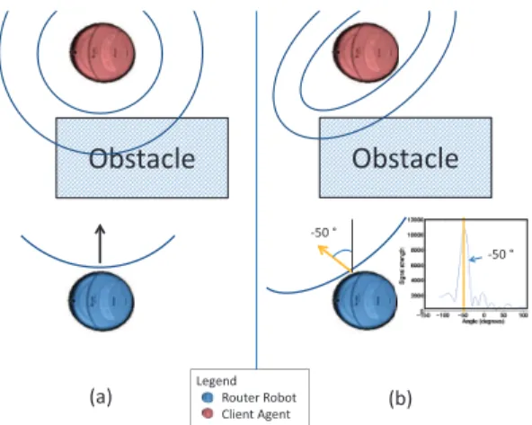
Obstacle

Obstacle

Fig. 6. Schematic depiction of the use of channel feedback for assigning cost to communication links in the network where edge cost is shown as circular contour lines. On the left, a Euclidean distance metric assigned lowest cost to the straight-line direction, whereas using the Mahalanobis distance (right)

skews the distance contours to identify the direction about~vθmaxas the lowest

cost. The amount of skew in the contour lines is determined by the confidence metric derived in Section V-B.

the Mahalanobis Distance between x and y is: distM(x, y) =

q

(x − y)T_{M(x − y) (9)}

Euclidean distance is a special case of the Mahalanobis

distance (see Fig. 9(a)) with M = I where I is the identity

matrix of appropriate dimension.

Here, M= QΛQT _{is a positive-definite matrix, where Q}

consists of orthogonal eigen-vectors and Λ contains their

corresponding eigen-values. By a careful construction of the matrix M, we can encode channel feedback as a quadratic Mahalanobis distance cost for each communication link in the network. This construction requires both the recommended

descent direction~vθmax from fi j(θ), and the confidence metric

σi j that is also computed from fi j(θ) in the following section.

B. Confidence Metric from Channel Feedback

We design a parameterσi j that is derived from the mapping

fi j(θ) and that we refer to as a confidence in the recommended

heading direction~vθmax. Intuitively,σi j captures the“variance”

of fi j(θ) around θmax. We define σi j mathematically as the

ratio of two quantities,σ_{f i j} andσ_{N i j}. We define

F=

∑

∑

∑

where L is the total number ofθ values that make up the plot

fi j(θ). The term σ_{f i j} is the variance of the plot fi j around

its maximumθ=θmax andσN i j is a normalization factor (it

is the variance around θmax in the case that the mass under

the fi j(θ) curve was distributed evenly over the θ values).

The ratio of these two quantities, σ_{f i j}/σN i j, characterizes

−6 −4 −2 0 2 4 6 −6 −4 −2 0 2 4 6 Ps= 0 Ck= 1 Ck= 2 0.1 0.51 10 10 10 10 25 25 25 25 25 25 50 50 50 50 50 50 50 50 100 100 100 100 150 X Y

Euclidean Distance Metric

(a)Euclidean Distance

−6 −4 −2 0 2 4 6 −6 −4 −2 0 2 4 6 Ps= 0 Ck= 1 Ck= 2 0.1 0.51 10 10 10 25 25 25 25 25 50 50 50 50 50 50 50 100 100 100 100 100 100 100 100 100 150 150 150 200 200 X Y

Mahalanobis Distance Metric Optimized Router Direction

(b) Mahalanobis (Low Conf) −6 −4 −2 0 2 4 6 −6 −4 −2 0 2 4 6 Ps= 0 Ck= 1 Ck= 20.51 10 10 25 25 25 25 50 50 50 50 50 100 100 100 100 100 150 150 150 150 150 150 200 200 200 200 200 200 X Y

Mahalanobis Distance Metric

(c) Mahalanobis (High Conf)

Fig. 9. These plots show the level sets of a Euclidean distance function and

a Mahalanobis distance function.

the amount signal strength (mass under the fi j(θ) curve)

that is concentrated under the peak direction θmax versus the

remaining parts of the curve. A ratio ofσ_{f i j}/σN i j= 1 would

mean that the fi j(θ) plot does not provide evidence that the

max directionθmaxis of much significance and that indeed the

plot is entirely noise. On the other hand a ratioσ_{f i j}/σN i j< 1

indicates that a significant portion of the signal strength curve

in fi j(θ) is concentrated around the max θmax and thus this

peak is considered to have “high confidence.” Lastly, the case

where σ_{f i j}/σN i j> 1 indicates the presence of high signal

strength in other parts of the fi j(θ) curve other than the

θmaxdirection which suggests the presence of multipath. These

three scenarios are demonstrated empirically in Figure 7 where

three actual fi j(θ) plots are automatically identified as being

single peak “high confidence”, multiple peak “noise”, and mul-tiple peak “multipath” scenarios respectively, by computing

the ratioσi j for each plot. The figure demonstrates a graphic

depiction of this ratio where areas of the fi j(θ) plot above

and below the uniform variance line determine the confidence value (compare with Equations in (10)).

We define these three cases below for reference:

Definition 2 (Confidence): Confidence in the direction of

highest signal strength θmax. We define three cases captured

by our confidence metricσi j=

σf i j σN i j:

• High confidence peak:σi j< 1

• Noise: σi j≈ 1

• Multipath:σi j> 1

See Figure 7 for examples of these regions identified automat-ically from actual experimental data.

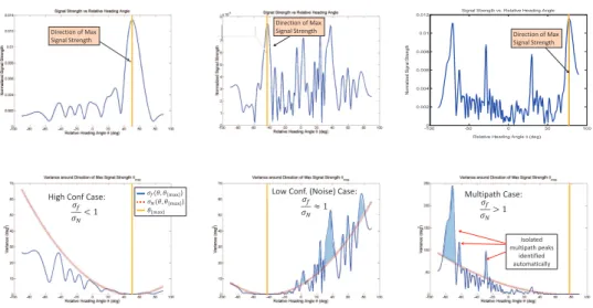
Experimental results in the basement of the Stata Center building on the Massachusetts Institute of Technology campus show that the regions of high confidence, noise, and multipath defined above can be identified automatically from data using the confidence metric from Eq. (13) (see Figure 8a). As ex-pected, areas of the environment with no significant occlusions to the client agent show strong evidence of high confidence profiles. Areas such as corridors with potential occlusions due to walls and corners show a much higher incidence of multipath, about 90% in the worst case.

Direction of Max Signal Strength Direction of Max Signal Strength -1000 -50 0 50 100 0.002 0.004 0.006 0.008 0.01 0.012

Signal Strength vs. Relative Heading Angle

Relative Heading Angle T (deg)

N o rm a liz e d S ig n a l S tr e n g th Direction of Max Signal Strength

High Conf Case:

ߪ௙

ߪே< 1

ߪ௙(ߠ, ߠ୫ୟ୶) ߪே(ߠ, ߠ୫ୟ୶) ߠ୫ୟ୶

Low Conf. (Noise) Case:

ߪ௙ ߪேൎ 1 Multipath Case: ߪ௙ ߪே> 1 Isolated multipath peaks identified automatically

Fig. 7. These plots show directional signal strength profiles from actual experiments. They demonstrate how the confidence metric identifies cases of high

confidence, low confidence, and multipath automatically from the fi j signal strength profile. The dotted red line is the variance,σN i j, of a uniform signal

strength profile fN i j(θ) = 1/L centered aroundθmax. Comparing the variance (bottom row)σf i jtoσN i jindicates which of the three cases are occurring in

the fi jplot (top row): high confidenceθmax(σ_{f i j}<σN i j), low confidence (noise)θmax(σ_{f i j}≈σN i j), or multipath aroundθmax(σ_{f i j}>σN i j).

2% 90% 8% 84% 8% 8% -100-80-60-40-20 020406080100 0 0.002 0.004 0.006 0.008 0.01 0.012 0.014

Sigma around thetaMax=0.496163 Iteration t=34 -1000 -80-60-40-20 020406080100 1 2 3 4 5 6 7 8 9x 10-3

Sigma around thetaMax=2.056633 Iteration t=53

(a) Confidence Metric

Client

Legend

Cost Contour High Confidence Cost Contour Low Confidence Control Input

Gradient Field using Gradient Direction and Confidence from Channel Feedback

Areas of multipath recognized and control action conservative along these directions

(b) Resulting Control Action

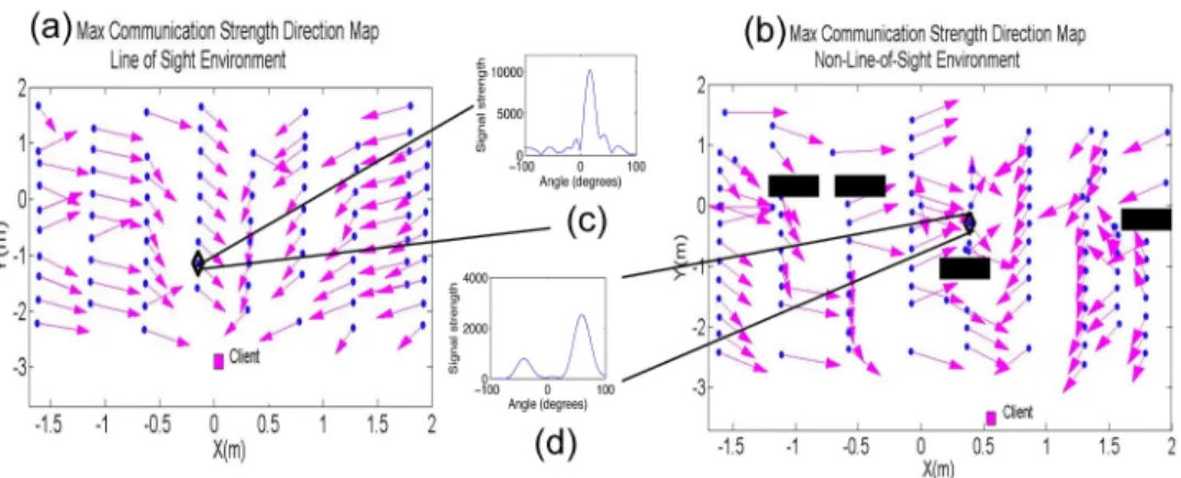
Fig. 8. Figure (a) shows data collected for a one-link system of one router and one client where the client is stationary at the top right corner of a basement

environment and a mobile router is driven in a lawn mower pattern throughout the environment through line-of-sight and non-line-of-sight regions. Each colored data point represents an acquired directional signal profile (two example profiles are shown) and the color of the data point is the result of automatic mode detection from the data using the confidence metric from Eq. (13) where red=noise, yellow=multipath, and green=high confidence peak. In (b) the resulting edge cost contours ( Equation (14)) and actual control command at each point in the environment is shown. Confidence values have a direct effect on velocity (as indicated by arrow length) where confident directions are pursued more aggressively.

An important observation from the data in Figure 8a is that even in line-of-sight regions of the environment (relative to the position of the client) there may be significant multipath present due to reflections from nearby concrete walls and this may cause the direction profile to have peaks in heading directions that are non-intuitive. Therefore this data suggests that metrics relying solely on the geometry of the environment, including visibility graphs, do not adequately capture the com-plexities of wireless signal quality in general environments. C. Construction of Communication Link Costs

Our objective here is to construct the Mahalanobis distance

matrix Mi j for each communication link (or edge) in the

network using fi j(θ). Specifically,

Problem 2 (Computation of Mi j): For each communication

link(i, j) in the network where i ∈ [k] and j ∈ [n], find a

head-ing direction~vθmax, a confidence metricσ, and a construction

of Mi j such that setting the edge costs ˜g from Equation (8) to

˜

g := dist2

Mi j(pi, cj) satisfies Properties 1-3.

The direction along which the signal strength is maximum,

θmax, is characterized by a peak in the fi j(θ) plot and we

define~v_θmax to be the unit vector along this recommended

heading direction θmax. Using this direction alone does not

provide enough information for effective position control of the routers however, due to the fact that this direction may experience corruption due to noise or multipath. In the previ-ous section we showed that the presence of multipath or noise

in the fi j(θ) plot can be identified via the computation of a

confidence metricσi j. Now, we encode the quantity σi j into

our controller such that~vθmax directions of high confidence are

followed more aggressively (larger displacements along these

directions), and the opposite is true of~v_θmax directions with

low confidence. Figure 8b shows the effect of the confidence value on the commanded displacements made by the controller

in an actual implementation.

Specifically, for the three categories of σi j we desire the

following behaviors for the routers: 1) σi j < 1: Indicates a

high confidence in~v_θmax due to a sharp peak in fi j. The robot

is moved at higher speeds; 2) σi j≈ 1: Indicates that fi j is

noisy, so the robot moves slowly; 3)σi j> 1: Indicates that fi j

has multiple significant peaks owing to multi-path. We study this last case in Sec. V-D., and particularly the opportunity it presents for making trade-offs between clients.

We use the heading direction and confidence to design a cost

function ˜g that locally captures the cost of communication in

the spatial domain. We express this cost as a Mahalanobis distance. The square of the Mahalanobis distance is a cost function (paraboloid) with ellipsoidal level sets (Fig. 9). We design our cost by orienting these level sets so that the

direction of steepest descent is along ~v_θmax. We then skew

the ellipsoidal level sets using the confidence σi j, so that a

higher confidence translates to a steeper descent which leads to larger router displacements (speed) in the descent directions with high confidence.

Algorithm 2 provides a calculation of the matrix Mi j from

Problem (2). We simply set one of the eigen-vectors of Q to

the heading direction~vθmax. To skew the ellipsoid, we set the

ratio of the eigen values{λ1,λ2} inΛ to the confidenceσ_{i j}2,

i.e. λ2/λ1=σi j2, where λ1 is the eigen-value corresponding

to~v_θmax. For example, in Fig. 9(b), where σi j≈ 1 (i.e. poor

confidence), the level sets are nearly circular, leading to a

shallow descent in cost; while Fig. 9(c), where σi j< 1 (i.e

high confidence), the level sets are skewed, leading to a steep

descent in cost along~v_θmax. In other words, the cost function

has an elegant geometric interpretation, akin to Euclidean distance, but is derived directly from channel measurements.

Further, the cost function ˜g := dist2

Mi j(pi, cj) from Eqn. 9 is

quadratic, a desirable property for optimizations.

Algorithm 2: Algorithm for constructing Mi jfrom channel

feedback.

input : Directional signal strength map fi j for every link

(i, j) from Algorithm 1

output: A matrix Mi j for defining communication edge

costs in Equation (8) using Mahalanobis distance from Problem 2.

1 Q_{i j}← [~v_θmax,~v_θmax⊥]// a set of orthonormal basis

vectors defined using~vθmax

2 σ_{i j}←σ_σf i j

N i j // confidence in the~vθmax direction

3 Λ= diag([ 1

σ2

i j

, 1]) // Construct a diagonal matrix

using confidence

4 M_{i j}= Q_{i j}ΛQT_{i j}

D. Network Trade-offs

In this section, we show how our optimization frame-work readily extends to a multi-agent scenario and study the different trade-offs. We show that via the setting of two parameters, both set automatically from wireless channel data, the resulting positional controller can be made to greedily optimize one client’s needs or alternatively, strike trade-offs between multiple clients. First, we focus on managing service

discrepancies specified by wi j. The quantity wi j aims to bias

the controller by assigning higher weight to users with larger service discrepancies. To do this, we scale the cost function

˜ g= dist2

Mi j(pi, cj) by the square of the discrepancy w

2

i j to

optimize yield the network cost:

rM(P,C) = max

pj∈P

min

ci∈C

{w2i jdist2Mi j(pi, cj)} (14)

Second, we highlight the subtle role played by the confidence

σi j in managing network trade-offs. For instance, consider a

scenario with two clients: 1 and 2, where client-1 demands

greater communication quality (as specified by wi j’s). Suppose

client-1 has a highly confident~v_θmax as shown in Fig. 10(a)

(i.e σi j < 1). As expected, the robotic router is directed

towards client-1 as shown in Fig. 10(c). In the more interesting scenario in Fig. 10(b), client-1’s confidence is poor due to

multiple peaks in the signal profile fi j (i.eσi j> 1). Here, the

router strikes a trade-off and services client-2 instead, as this may potentially benefit client-1 as well due to the multipath

recognized in client-1’s fi j(θ) map. The intuition behind this is

simple. Equation 14 above, scales the ellipsoidal cost function

based on the discrepancies wi j’s. However, recall that the

ellipsoidal cost function is steep (or shallow) depending on whether the confidence is high (or low) and this is attained

by setting the ratio of eigenvaluesλ2/λ1 of Mi j (See Line 3

in Algorithm 2). In extremely low confidence scenarios such as Figure 10(b), the higher value of discrepancy of client-1 is masked by its low value of confidence. Hence, this balances the trade-off in favor of client-2, despite having a lower discrepancy. −1000 −50 0 50 100 2000 4000 6000 8000 10000

Relative Heading Directions of Max Signal Strength High Confidence Single Direction

Relative Heading Theta (deg)

Signal Strength (dB)

(a) High Certainty Direction

−1000 −50 0 50 100 1000 2000 3000 4000 5000 6000

Direction of Max Signal Strength with Multipath

Relative Heading Theta (deg)

Signal Strength (dB) (b) Multipath Directions −6 −4 −2 0 2 4 6 −6 −4 −2 0 2 4 6 Ps= 1 Ps= 2 Ck= 1 Ck= 2 0.1 0.5 1 10 10 25 25 25 50 50 50 50 100 100 100 100 100 150 150 150 200 200 200

High Priority Sensor

X Y 0.50.1 1 1 10 10 10 25 25 25 25 25 50 50 50 50 50 50 100 100 100 150 150 150 150 200

Medium Priority Sensor

Optimized Router Direction in Favor of High Priority Sensor with Large Certainty

Optimized Router Direction

(c) Client Favored −6 −4 −2 0 2 4 6 −6 −4 −2 0 2 4 6 Ps= 1 Ps= 2 Ck= 1 0.1 0.5 1 1 10 10 10 25 25 25 25 50 50 50 50 50 50 100 100 100 150 150 150 200

High Priority Sensor

X Y 0.1 0.5 1 1 10 10 10 25 25 25 25 50 50 50 50 50 100 100 100 150 150 150 200 200

Medium Priority Sensor Mobile Router Direction Optimizes Competing Demands

by Recognizing Multiple (Multipath) Directions

Optimized Mobile Router Direction

(d) Client Tradeoff Multipath

Fig. 10. Trade-offs between Clients: (a) − (b) show the fi j(θ) map for the

high demand client;(c) − (d) show the optimized router direction

Algorithm 3 demonstrates how the cost in Equation (14) can be used to find an updated set of router positions when both client and router positions are known at the current iteration. The optimization in Equation (15) in Algorithm 3 is equiv-alent to a k-center optimization problem where the distance metric is a Mahalanobis distance. This is a generalized router placement problem similar to that studied in [Gil et al., 2012] for Euclidean distances. Thus the returned solution from this algorithm is the optimal placement of routers corresponding to

the optimal assignment of routers to clients, given the channel feedback at the current iteration t.

Algorithm 3: Algorithm for router placement with known client positions.

input : Directional signal strength map fi j(θ) for every

link(i, j), demand qj, relative importanceαj> 0

for client j, current quality of each linkρi j, and

current router and client positions P= {p1, . . . , pn}, C = {c1, . . . , cn}

output: A configuration of optimal router positions C∗,

|C∗| = k, given the current channel feedback for

all links in the network.

1 for all links (i, j) in the network withρ_{i j}> 0,

i∈ [k], j ∈ [n] do 2 w_{i j}← max(α_jqj−ρi j qj , 0); 3 Mi j← result of Algorithm 2; 4 end 5 Compute: C∗= arg min C {maxpj∈P min ci∈C w2_{i j}(pi− cj)TMi j(pi− cj)} (15) return C∗ E. A Position-Independent Solution

A simple relaxation to the cost from the previous section frees the optimization of using client positions, while main-taining its simple structure and desirable properties developed

above. Consider a user specified step-sizeγ> 0, that encodes

the maximum permissible displacement for each router and

denote ci,t to be the current router position. We replace client

positions pj in Equation (14) with “virtual” positions p′i j:

p′_{i j}= ci,t+γwi j~vθmax. (16)

Intuitively, a client is no longer directly observed but rather

estimated to be along the relative direction ~vθmax and at a

distance ofγwi jwith respect to the ith router. As before,~vθmax

is the heading direction associated with the maximum strength

signal directionθmax. As a client’s demand is better satisfied

by router i, the service discrepancy wi jtends to 0 and the client

is perceived as being closer to router i. The observation here is that routers better equipped to service a particular client as

reflected by the wi j term, will view the client as “closer” and

those routers with a weaker signal to the same client will view this client as farther away. This results in a natural method of assigning client nodes to routers by effectively sensing over the wireless channels.

F. Controller for Router Positioning

We now present an algorithm for achieving router positions

that minimize the edge costs ˜g derived in the previous sections.

Particularly we formulate ˜g from Equation (3) to be

˜

g(ci,Ct, wi j, fi j) = (p′i j− ci)TMi j(p′i j− ci) (17)

Where the dependence of ˜g on Ct, wi j and fi j are captured

indirectly by p′_{i j} and Mi j via Equation (16) and Algorithm 2

respectively. This choice of edge costs satisfy Properties 1-3. Namely, having a quadratic form, allowing optimization over the entire network with competing demands, and being independent of client positions. As described in Section III, minimization of these edge costs by Equation (3) results in the optimization of a network-wide metric, ie. minimizing the worst-case client service discrepancy.

The resulting optimization framework can be shown to exhibit other desirable properties relative to the instantaneous wireless channels over the network. An important remark is that we do not make assumptions on how the wireless channels may change over time, nor do we make assump-tions on the underlying signal quality function in areas of the environment that are not currently being sensed by the routers. Unfortunately, this impairs our ability to prove certain desirable controller attributes such as convergence, that would require some additional assumptions on the signal quality such as a guarantee that this function is smooth, and can be strictly improved at every iteration. Such assumptions would be invalidated by small-scale fading alone [Goldsmith, 2005; Lindhe et al., 2007] , in real wireless systems. How-ever, by relying solely on instantaneous channel feedback, we retain the important ability to adapt quickly to changes in the wireless environment due to dynamic obstacles, for example. Based on current channel feedback, we highlight our controller’s network-wide properties. The following properties, and convergence to client demanded rates, are demonstrated extensively in actual implementations in the next section of the paper:

Property 4: The assignment of routers to clients is optimal based on the current feedback over wireless links in the network.

This can be seen from the observation that Line 8 from Algorithm 4 is the classic k-center solution [Feldman et al., 2013; Gil et al., 2012] under the Mahalanobis distance metric. A k-center solution will assign clients to their closest routers. In this case “closest” is defined in the signal quality sense where routers serve the clients to whom their signal strength is greater than the signal strength between any other router in the network to the same client. An example of this property in an actual hardware implementation can be seen in Section VI-C-VI-D where routers choose clients based on the strengths of their relative wireless links.

Property 5: Stability of router positions to solutions that satisfy client demands over the network.

Our final cost takes the form:

rM(C) = max

j∈{1,...,n}minci∈C

{dist2

Mi j(ci,t+γwi j~vθmax, ci)} (18)

By expanding the squared per-link cost dist2_M

i j(ci +

γwi j~vθmax, ci) from Eqn. 14:

(ci− ci,t)TMi j(ci− ci,t) − 2γwi jλθi j~v T θmax(ci− ci,t) +γ 2_w2 i jλθi j (19)

we note that as wi j→ 0 the first term in Eqn. (19) favors stable

solutions where ci= ci,t, ie. the router reaches a static solution

when all of its assigned clients have zero service discrepancy. In the case where it is not possible to satisfy all client demands, for example if there are not enough routers k to provide communication coverage to the clients, Algorithm 4 returns the solution with the lowest service discrepancy that is within a user specified tolerance of optimal. Extensive empirical