OpenComp3d: An open-source framework dedicated to design in power electronics

(1)

HAL Id: hal-02403665

https://hal.archives-ouvertes.fr/hal-02403665

Submitted on 2 Dec 2020

HAL is a multi-disciplinary open access

archive for the deposit and dissemination of

sci-entific research documents, whether they are

pub-lished or not. The documents may come from

teaching and research institutions in France or

abroad, or from public or private research centers.

L’archive ouverte pluridisciplinaire HAL, est

destinée au dépôt et à la diffusion de documents

scientifiques de niveau recherche, publiés ou non,

émanant des établissements d’enseignement et de

recherche français ou étrangers, des laboratoires

publics ou privés.

OpenComp3d: An open-source framework dedicated to

design in power electronics

A. Morentin, G. Fontès, Miguel Mannes Hillesheim, Thierry Meynard, D.

Flumian, J. Bourdon, H. Piquet

To cite this version:

A. Morentin, G. Fontès, Miguel Mannes Hillesheim, Thierry Meynard, D. Flumian, et al..

Open-Comp3d: An open-source framework dedicated to design in power electronics. Mathematics and

Computers in Simulation, Elsevier, 2019, 158, pp.477-489. �10.1016/j.matcom.2018.11.006�.

�hal-02403665�

(2)

OpenComp3d: An open-source framework

dedicated to design in power electronics

A. Morentin

∗

_{, G. Fontes, M. Mannes Hillesheim,}

T. Meynard, D. Flumian, J. Bourdon,H. Piquet

Laplace, University of Toulouse, 2 rue C. Camichel, Toulouse, France

Abstract

This paper is an overview of an innovative optimization framework developed for the design of power converters, which is available under MIT licence in a github repository (https://github.com/Laplace-cs/OpenComp3d). In the first part, the general principles, structure and standards are presented. In the second part, an example is performed to optimize the output inductor of a buck converter showing the advantages of the proposed methodology.

Keywords: Software prototyping; Power electronics optimization

1. Introduction

As electric energy management provides high efficiency conversions, power converters are more and more used in stationary or embedded applications. The design of these power converters is thus an important challenge in industrial field: they are complex systems, the prototype building is usually expensive and the design mainly relies on the engineer experience of this field.

Designers choose between a series of different components, topologies, control laws etc. to create a product fulfilling the expected performance and the specifications. In addition, the characteristics of the electrical equipment (lower mass, volume, cost and higher efficiency and reliability) must be improved.

As these converters manage energy flows, looking for the maximum efficiency leads to design conversion systems with minimal power density: i.e. conversion systems whose size tends towards infinity. Thus, designers have to find solutions with best compromise between efficiency and compactness (mass, volume) of the power converters.

Today, generic or very specific analysis software are available for power electronic designers, but they only answer partially or locally to their needs. Few software tools in the domain of power electronics can really assist them in the “operational” steps of conception such as design or optimization. The need of new tools has been clearly stated several times [8,11].

(3)

For example, in [1], a design environment is presented to design a single-phase PFC converter. In [5], an optimization framework called CADES (Component Architecture for Design of Engineering Systems) is presented to perform an optimized system design. Predictions estimate that in 2020, 80% of the design process will be performed by computers [11]. New companies are arising and proposing software solutions (e.g. PowerForge [17] or GeckoSimulations [10]) to the new problematic.

The work presented in this paper is in the field of “virtual prototyping” for power electronics: a framework which can be considered as a “design environment” to perform the design process of power converters.

2. Framework concept

Different modelling languages are already used for the design step in the industry, such as Modelica [14] or SysML [19]. However, they cannot be directly used as design frameworks in power electronics: SysML is a description language and does not itself provide any solver to simulate the whole model; Modelica also requires a specific compiler not subject to free licence agreements.

The developed framework OpenComp3d provides a three-dimensional physical description pattern of power components. The framework is available under a MIT licence in a github repository (https://github.com/Laplace-cs/ OpenComp3d). It uses an object-oriented programming approach, implemented in Matlab⃝R _{. The description} pattern implies that each component is coded as an object with some characteristics or properties and some mathematical functions or methods to calculate the different data of the component. The calculation process behind every object of the framework is presented in Fig. 1.

From the inputs (physical dimensions, material and shape), the parameters (mass, volume and cost) and the equivalent simulation models (electric, magnetic and thermal) are extracted. This way of describing models is called “direct modelling” and is characterized by the unicity of the solution. Furthermore, external excitations (voltage, current and magnetic waveforms) provide additional information (losses, temperatures, magnetic field etc.) to ensure proper design of the components.

In the framework, objects or components are grouped in different categories or families depending on their function, materials, etc. Therefore, a tree class is created to group the elements that share certain properties or methods. For example, all magnetic components (inductors, transformers, etc.) share the core and winding material

properties and the methods to calculate the core losses.

In addition, in the tree class, abstract classes are introduced to define a standard that all components inserted in the library must respect. The standard is important for incremental development of the framework. It helps understanding models developed by other designers and eases the use of implemented code.

At the top of the tree class (See Fig. 2) is situated the abstract class Component that contains the abstract properties (geometric data, electric data for example) and methods (display methods, parameter computation).

(4)

A. Morentin, G. Fontes, M.M. Hillesheim et al. / Mathematics and Computers in Simulation 158 (2019) 477–489 479

From this class, two abstract classes are derived:

• Element: is the mother class for every physical device and contains all shared properties (shape, dimensions and material) specific to the “direct modelling” approach. From this class derive devices such as inductors, capacitors, heat sinks etc.

• Composite: is the mother class for any device which is formed by the association of Elements. For example, a LC filter is formed by the association of an inductor Element and a capacitor Element.

Below these two main classes, additional abstract classes are derived as well, such as a magnetic class to pool the different magnetic components (inductor, transformer etc.). The main objective is to define the different functions only once in the environment. Code implementation repetition is avoided and bug fixing becomes less tedious. For example, a transformer model derives from the magnetic abstract class and benefits from the core loss density method of the abstract class. The tree class was conceived as well to anticipate future developments. More details are available in the framework documentation in the github repository ( https://github.com/Laplace-cs/OpenComp3d).

3. Setting the environment

As presented in Fig. 1, the models require an “excitations” input representing the waveforms each component is withstanding. The excitations are determined in two different ways: analytically or using an external solver.

3.1. Analytical

In some basic topologies (e.g. an output inductor of a buck converter) the “excitations” are defined by simple equations. The computation time as a consequence is very short. However, this method requires a definition for each topology and is often based on some hypothesis, thus restraining the domain of exploration.

3.2. External solver

The different equivalent circuits of each component are sent to a circuit solver to calculate the different waveforms. In the design example of this paper (Section 7), a frequency solver called OOTEE [6] (developed by the LAPLACE laboratory) is used and offers a good trade-off between computation time and precision (Fig. 3).

(5)

For example, to calculate the steady-state of a three-phase inverter, the frequency solver provided a simulation time of 0.15 s compared to a time-domain solver with a convergence accelerator (the steady state analysis tool of Plecs⃝R

in this example) with a simulation time of 1.24 s for the same circuit. The comparative of the output current for the two simulation solvers is shown in Fig. 4. For this waveform, the mean error is calculated at 0.28 A (0.37% relative) and the maximal error is 0.7 A (1.74% relative).

The frequency solver has other advantages such as simulating frequency behaviour (e.g. skin effect on windings) or filter design. Indeed, only the frequencies of interest can be simulated which is particularly interesting for commonmode simulation.

The solvers (Ex. OOTEE, etc.) are strictly out of the framework scope and users may want to test different commercial packages (Plecs⃝R _{, etc.). As a result, the interfaces have been defined to couple the models to different} simulation solvers. These include some definitions of the equivalent lumped models and the acceptance of waveforms under certain formatting rules (Ex. Fixed-step waveform data etc.).

4. Optimization

So far, the design pattern to model the components and how to use them with different solvers has been presented. The designer changes the different inputs (dimensions, materials, shape...) and looks if the proposed solution satisfies the specifications. This process becomes tedious and the “optimality” of the solution is non-guaranteed and highly-dependent on the designer’s expertise. OpenComp3d overcomes this limitation by proposing an optimization environment that chooses under a certain criteria (mass, volume, efficiency or combination of them) which are the best inputs.

A library of different optimization methods are defined in the framework to minimize the objective function (mass, cost, losses, volume). In the current version of the open-source framework, the only available optimization

(6)

algorithms are the ones proposed by Matlab⃝R _{. However, the objective is that the different developers may include} their optimization algorithms in the framework and see how they work in different design problems. Moreover, specific routines are created to decouple the mathematical optimization problem from the component models. As a result, the users may easily plug their models in the framework and take advantage of the created optimization routines.

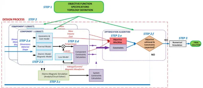
Fig. 5. Optimization algorithm process.

5. Final validation

Once the optimal solution has been found, a validation still needs to be performed. The validity of the analytic model in the whole exploration area is not guaranteed and therefore a numerical simulation must be done at the end. If the error is below a certain threshold, the solution is accepted and if not, the model needs to be modified to increase its accuracy in this particular region. Numerical simulations are the most accurate calculations that can be performed before experimentation, thus reducing the risk of non-compliance in the final prototype.

The whole design process is described in Fig. 5 which is a schematic of what was previously explained and involves the following steps:

• step 1 corresponds to the description of the problem: function to optimize, specifications or constraints of the problem and the circuit topology,

• step 2 describes the whole design process,

◦ steps 2.a-d show the interaction between the solver and the different components (Section 3) ◦ steps 2.e-f describe briefly the use of the optimization algorithm (Section 4),

• step 3 the numerical simulation is performed to accept the solution.

The whole environment has been deployed using Matlab⃝R _{software. There are only two steps where other} softwares might be used: solver and final validation. However, in those cases the launch will be sent from Matlab⃝R . This is not a drawback since a large part of the candidate software already provides routines to interface with Matlab⃝R _{(e.g. Comsol}⃝R _{, Plecs}⃝R _{, Femm}TM_{, etc.).}

6. Sweep tool

The framework provides as well a sweep tool to evaluate the influence of different inputs (e.g. to test the reduction of thermal resistance when adding another fin in a heatsink) and find the best values in terms of mass,

(7)

efficiency, etc. or find the feasible components under certain conditions. This is particularly useful when some environmental conditions (such as thermal conditions) are uncertain. The user may want to look what will be the impact of the uncertainty about a parameter in the final solution.

The sweeping tool has been developed under Matlab⃝R _{and is a layer that provides shortcuts to evaluate models} in different points and plotting functions. The sweeping tool can also be used in the optimization process to assess the impact of some parameters (e.g. filter mass sensibility with switching frequency) as will be shown in the design example.

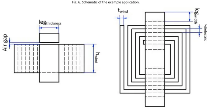
Fig. 6. Schematic of the example application.

Fig. 7. Dimensions of the inductor.

7. Design example

To illustrate the use of this framework, let us consider the design of the output inductance of a buck converter as shown in Fig. 6.

7.1. Description of an inductor

In the example, the inductor is composed by the association of an E-I core and a foil winding. The materials are

Ferrite N87 for the core and copper for the winding and are set at the beginning of the optimization process. The

inductor is defined by inputs/dimensions shown in Fig. 7 that are as well the optimization variables of the problem. These inputs are:

• leg width, • leg thickness, • height winding,

(8)

• thickness winding,

• number of turns, • thickness dielectric, • air gap.

In this case the objective function is to minimize the mass of the inductor which is directly calculated from the volumes

(calculated from the dimensions Volcore,Volwinding) and the materials densities (ρcore, ρwinding)

min (Volcore · ρcore + Volwinding · ρwinding) (1)

7.2. Electrical excitations 7.2.1. Electromagnetic model

As all the components in the framework, the inductor has an equivalent electrical simulation model to extract the different waveforms. This equivalent model will be used in this case with the OOTEE solver as presented in Section 3.2 to extract the current of the inductor. In our case, an equivalent lumped model using the inductor permeance representation [2,4] is used (see Fig. 8). In this representation, the magnetomotive force (mmf) is an image of the current I and the magnetic flux derivate φ˙ is an image of the voltage V.

V

φ˙ = (2)

N

mmf = N · I (3)

The magneto-electric coupling is simulated by an equivalent transformer model [2,4]. Moreover, the relationship between these two magnitudes is associated to an inductor whose permeance value P is equivalent to:

µ0µr Ae

P = (4) l

With µ0 the air permeability, µr the relative permeability, Ae the magnetic cross-section area and l the magnetic path

length of the permeance section.

The inductor value L is calculated by the sum of all the permeance values.

N2µ0Ae

L = (5)

∑ P−1

With N the number of turns. The magnetic field B is extracted from the excitations. The maximum of this magnetic field must be below the saturation field of the magnetic material Bsat. The design limitation is considered as a

(9)

constraint in the optimization problem. A margin of 0.95 is applied to ensure operation in the linear magnetic part of the material B-H curve.

g(x) = B − 0.95 · Bsat ≤ 0 (6)

7.2.2. Core losses

From the magnetic field waveform B, the core losses are calculated using the iGSE model [20], which is a fair core loss calculation for any type of waveform.

Pc = Vol · i

⏐ ⏐ dt(7)

k

ki (8)

With Pc the core losses, Vol the volume of the magnetic core, T the period and k, α, β the Steinmetz coefficients. The

Steinmetz coefficients are directly obtained from the material datasheet which is an advantage for the design

Fig. 9. Comparison of optimal results with classical product area versus current ripple [15].

framework as any user can easily include the materials he may particularly be interested in. On the other hand, this method has the limitation of not including the relaxation or DC bias effects in the loss calculation [16,18].

7.2.3. Winding losses

The Joule losses are calculated using the RMS current value Irms obtained from the simulations.

Pj = (F + G) · RDC · Irms2 (9)

With RDC the DC resistance of the inductor and F, G correction coefficients to take into account the skin and proximity

effects respectively. These coefficients are usually calculated with analytic expressions, mostly based on the “Dowell” formula [7]. However, these expressions have usually a restrained acceptable validity region, especially for the proximity effect, where the magnetic field in the window of the inductor needs to be determined [9,21].

To solve these limitations, in this model, a large number of 2-D numerical simulations have been performed and for each simulation F (skin effect) and G (proximity effect) correction coefficients have been extracted [3,15]. The simulations include all the variables influencing the two frequency effects. For example, for the skin effect these variables are:

(10)

• frequency, • height of the foil, • width of the foil,

• resistivity of the material.

From the data set of simulations, the missing regions are extracted by linear interpolation. The data is disposed in a grid form to reduce the interpolation computation time, thus all the combinations between the different variable values are calculated. Calculating all the combinations becomes a serious drawback when a lot of variables are involved and it is a point to be improved in future developments of this model.

The interpolation method (x) is compared to the classical Dowell formula (o) and Finite-Element Method (FEM) simulations with FEMMTM _{in two different geometries (see}_{Fig. 9}_{). For these two examples, the worst-case relative} error of the interpolation error is found at 26% while Dowell formula gives a maximal relative error above 1000% (for cases where a large airgap is close to the winding). Furthermore, what it is important is that both curves follow the same pattern meaning that sensitivity analysis will be representative of the real physics.

7.3. Thermal calculation

Calculation of temperatures in magnetic elements is a key factor in the design as they must be kept below certain material temperature limits. However, evaluation of the thermal performance of an inductor is a complex task. First,

Fig. 10. Inductor thermal model representation.

the geometry is complex and semiempirical formulations cannot be applied to estimate external convection exchange coefficients. Secondly, the thermal characteristics of the different materials are dissimilar. The winding behaves as a thermal conductor while the magnetic core and the dielectric behave as thermal insulators.

In our case the thermal behaviour of the inductor is modelled using 21 nodes as shown in Fig. 10. The three heat transfer mechanisms are considered: conduction, convection and radiation.

For the conduction, the classical formulation is used for the resistance between two nodes i and j:

(11)

With d the distance between nodes, k the thermal conductivity and At the distance between nodes. For the thermal

convection resistance between two nodes:

(Rthconv)ij = h · 1Aext (11)

where Aext is the external surface of the node and h the equivalent convection heat exchange coefficient. In our case,

a constant factor of 10 W/(m2_{K) is considered as a representative order of magnitude for natural convection. Yet, to} overcome this choice as well as the simplicity and inaccuracy of the thermal model, the optimization will be calculated varying this factor h of +−20% (i.e. 8 and 12 W/(m2_{K)). For the radiation thermal resistance the following} approximation is used:

≈ ε · σ · Aext

(Rthrad )ij

1 Text) (12)

With ε the material emissivity, σ the Boltzmann constant, Text the external temperature and Ts the surface

temperature. As presented, the thermal resistance depends on the surface temperature which is unknown. An iterative algorithm is employed where the radiation equivalent thermal resistance is reconsidered at each iteration. Another hypothesis of our thermal model is that loss density is constant at each part. The losses that must be evacuated at each node are:

Q = q˙ · Vol (13)

With Q the power losses, q˙ the loss density of the core or the winding and Vol the volume of the node. Once all the thermal resistances and power sources values are determined, a linear system of equations is obtained:

[1_/_R

th][T] = [Q] (14)

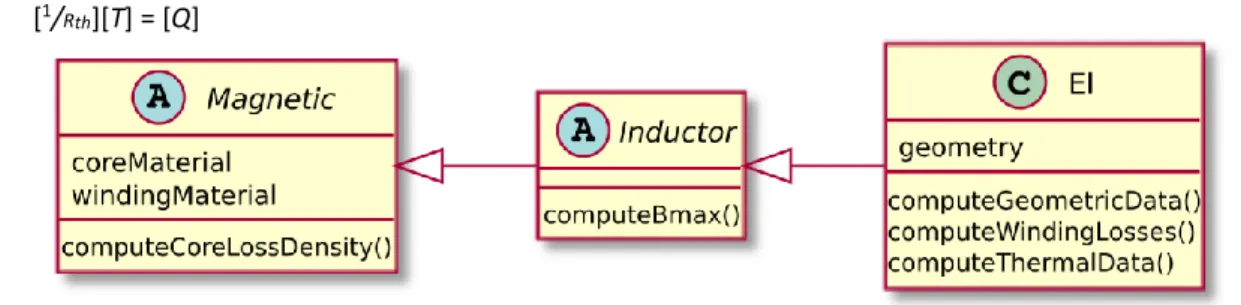
Fig. 11. UML non-exhaustive representation of the EI inductor implementation.

where T is the vector of the unknown temperatures to be determined. This system is solved with an external temperature Text (fixed at 25 ◦C) and the maximal temperature of the inductor is estimated. It must be kept below a

certain limit Tlimit (100 ◦C in our case) and is specified as a constraint in our optimization problem.

g(x) = max([T]) − Tlimit ≤ 0 (15)

7.4. Implementation

The implementation is done profiting from the architecture of the tree class presented in Section 2. The calculations that can be mutualized are included in top class. For example, the iGSE method can potentially be used by other magnetic components (e.g. Transformers) and therefore is included in the Magnetic class. The calculation of the total mass depends on the geometry and is therefore only implemented in the EI class. A non-exhaustive representation of the tree class and the implementations of the equations discussed earlier is presented in Fig. 11.

(12)

7.5. Optimization

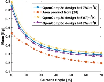
The optimization is performed using the gradient-type interior-point algorithm of Matlab⃝R _{because of its lower} memory usage [12]. For the initial points, 50 points are chosen with the Multi-Start algorithm. A sensitivity study using the sweeping tool (Section 6) is also performed to assess the mass of the inductor when ranging from 10% to 70% ripple of the load current. The following constraint is added to the optimization problem:

g(x) = ∆I − ∆Imax ≤ 0 (16)

To estimate the gain of the proposed approach, the results are compared to an analytical approach described in [13]. This approach first uses an area product (AwAc) calculation which takes into account frequency effects on

copper losses and a limitation of the alternative induction Bac to limit core losses and then determines a shape and

its dimensions to minimize the weight of the inductor. This direct calculation only uses loss densities and does not directly perform any calculations of the temperatures.

L · Iˆ · Irms

Ac · Aw = (17) kw · Jrms · Bac

With L the inductance value, Iˆ and Irms the maximal and RMS values of the current, kw the winding filling factor and

Jrms the current density in the winding.

The results are shown in Fig. 12. They show how using a more realistic thermal model changes the solution compared to an analytic approach. In addition, the variations on the thermal exchange coefficient bind the final mass between −5% and 6.3%. Therefore, the uncertainty of the thermal exchange coefficient can be easily compensated by a slight increase of the thermal exchange surface and consequently the mass.

7.6. Validation

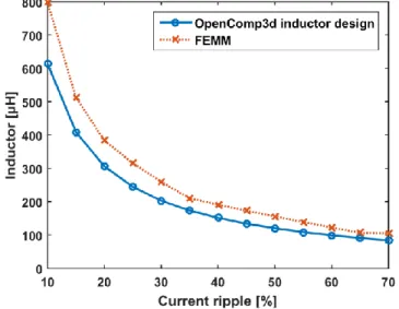
The optimal solutions are compared to 2D-numerical simulations with FEMMTM _{software to show validity of the} analytic formulas at the optimal points. In this case, the inductance value and the winding losses are compared (see

Figs. 13 and 14).

(13)

Fig. 13. Comparison between the analytical model and FEMM calculations for the inductance value.

For the inductance value, the analytic model underestimates the inductance because it does not consider the leakage inductance, therefore a margin is still exploitable to reduce the mass.

In the case of the winding losses, the results show a good accuracy of the losses (average error about 6%) and a light over-estimation meaning the solution is feasible and a certain mass margin is still exploitable. Further developments should include the thermal validation of the model as it has a direct impact on the final mass.

8. Conclusions

In this work, the methods and principles of a power converter design framework have been described. In this framework an innovative formalism is defined. The objective of this formalism is to provide an environment where several users:

• plug and share their models to avoid work repetition,

• choose different complexity levels of their models depending on what they need to focus on.

(14)

The framework can also be coupled with a fast-computation solver to get steady-state waveforms and with a library of optimization algorithms. Parametric or sensibility study methods are also implemented and allow the users to study the influence of variable external conditions (such as ambient temperature) or other robustness problems. At the end of this paper, an example of optimized design of the output inductor in a buck converter shows the customization potential of this new tool compared to classical approaches.

9. Perspectives

The perspectives of this work are infinite. For now, only the basis of a new design environment have been set. Our aim is to provide this open-source framework to a large community of users to enlarge the number of models, optimization algorithms. etc. This framework will serve as a common language for the different specialists of the power converter design and thus improving the design of power converters.

References

[1] J. Biela, U. Badstuebner, J.W. Kolar, Impact of power density maximization on efficiency of DC-DC converter systems, IEEE Trans. Power Electron. 24 (1) (2009) 288–300.

[2] J.C. Brandelero, Conception et Réalisation d’un Converteur Multicellulaire DC/DC Isolé pour Application Aéronautique (Diss.), INP Toulouse, 2015.

[3] R.M. Burkart, H. Uemura, J.W. Kolar, Optimal inductor design for 3-phase voltage-source PWM converters considering different magnetic materials and a wide switching frequency range, in: Power Electronics Conference (IPEC-Hiroshima 2014-ECCE-ASIA), 2014 International, 2014, pp. 891–898.

[4] E.C. Cherry, The duality between interlinked electric and magnetic circuits and the formation of transformer equivalent circuits, Proc. Phys. Soc. Sect B 62 (12) (1949) 101–111.

[5] B. Delinchant, D. Duret, L. Estrabaut, L. Gerbaud, H. Nguyen Huu, B. Du Peloux, H.L. Rakotoarison, F. Verdiere, F. Wurtz, An optimizer using the software component paradigm for the optimization of engineering systems, COMPEL - Int. J. Comput. Math. Electr. Electron. Eng. 26 (2) (2007) 368–379.

[6] Dépôt à l’Agence de Protections des Programmes: IDDN.FR.001.360033.000.S.P.205.000.20600.

[7] P. Dowell, Effects of eddy currents in transformer windings, Proc. Inst Electr. Eng. 8 (1113) (1966) 1387, 1394.

[8] U. Drofenik, D. Cottet, A. Müsing, J.W. Kolar, Design tools for power electronics: trends and innovations, Ingenieurs l’automobile 791 (2007) 55–62.

[9] J.A. Ferreira, Improved analytical modeling of conductive losses in magnetic components, IEEE Trans. Power Electron. 9 (1) (1994) 127–131. [10] Gecko-Simulations software. http://gecko-simulations.com/.

[11] J.W. Kolar, What are the “Big CHALLENGES” in Power Electronics?. (2014). [12] MATLAB Documentation https://fr.mathworks.com/help/matlab/.

[13] T. Meynard, Analysis and Design of Multicell DCDC Converters using Vectorized Models, John Wiley & Sons, 2015. [14] Modelica. https://www.modelica.org/.

[15] A. Morentin, Methods and Tools for the Optimization of Modular Electrical Power Distribution Cabinets in Aeronautical Applications (Diss.), INP Toulouse, 2017.

[16] J. Mühlethaler, Modeling and Multi-Objective Optimization of Inductive Power Components (Diss.), ETH Zurich, 2012. [17] PowerForge software. https://powerdesign.tech/powerforge/.

[18] M.S. Rylko, Magnetic materials and soft-switched topologies for high-current DC-DC converters. (2011). [19] SysML. http://www.omgsysml.org/.

[20] K. Venkatachalam, C.R. Sullivan, T. Abdallah, H. Tacca, Accurate prediction of ferrite core loss with non-sinusoidal waveforms using only Steinmetz parameters, in: Computers in Power Electronics, 2002. Proceedings. 2002 IEEE Workshop on, 2002, pp. 36–41.

[21] P. Wallmeier, N. Frohleke, H. Grotstollen, Automated optimization of high frequency inductors, in: Industrial Electronics Society, 1998. IECON’98, Proceedings of the 24th Annual Conference of the IEEE. Vol. 1, 1998, pp. 342–347.