HAL Id: hal-00452243
https://hal.archives-ouvertes.fr/hal-00452243
Submitted on 1 Feb 2010HAL is a multi-disciplinary open access archive for the deposit and dissemination of sci-entific research documents, whether they are pub-lished or not. The documents may come from teaching and research institutions in France or abroad, or from public or private research centers.
L’archive ouverte pluridisciplinaire HAL, est destinée au dépôt et à la diffusion de documents scientifiques de niveau recherche, publiés ou non, émanant des établissements d’enseignement et de recherche français ou étrangers, des laboratoires publics ou privés.
River model calibration, from guidelines to operational
support tools
Jean-Philippe Vidal, Sabine Moisan, J.B. Faure, Denis Dartus
To cite this version:
Jean-Philippe Vidal, Sabine Moisan, J.B. Faure, Denis Dartus. River model calibration, from guide-lines to operational support tools. Environmental Modelling and Software, Elsevier, 2007, 22 (11), p. 1628 - p. 1640. �10.1016/j.envsoft.2006.12.003�. �hal-00452243�
Author-produced version of the article published in Environmental Modelling and
Software, 2007, 22 (11), 1628-1640.
The original publication is available at http://www.sciencedirect.com/
doi : 10.1016/j.envsoft.2006.12.003
River model calibration, from guidelines to operational support tools
Jean-Philippe Vidal*
Cemagref, Hydrology-Hydraulics Research Unit, 3 bis quai Chauveau, CP 220, 69336 Lyon Cedex 09, France. Now at HR Wallingford, Water Resources Department, Howbery Park, Wallingford, OX10 8BA, United Kingdom
Sabine Moisan
INRIA, Orion Project, 2004 route des Lucioles, BP 93, 06902 Sophia-Antipolis, France
Jean-Baptiste Faure
Cemagref, Hydrology-Hydraulics Research Unit, 3 bis quai Chauveau, CP 220, 69336 Lyon Cedex 09, France
Denis Dartus
IMFT, Hydre Group, Allée du professeur Camille Soula, 31 400 Toulouse, France
* Corresponding author. Tel: +44 1491822338; fax: +44 149183635; E-mail address: [email protected]
Abstract
Numerical modelling is now used routinely to make predictions about the behaviour of environmental systems. Model calibration remains a critical step in the modelling process and different approaches have been taken to develop guidelines to support engineers and scientists in this task. This article reviews currently available guidelines for a river hydraulics modeller by dividing them into three types: on the calibration process, on hydraulic parameters, and on the use of hydraulic simulation codes. The article then presents an integration of selected guidelines within a knowledge-based calibration support system. A prototype called CaRMA-1 (Calibration of River Model Assistant) has been developed for supporting the calibration of models based on a specific 1D code. Two case studies illustrate the ability of the prototype to face operational situations in river hydraulics engineering, for which both data quality and quantity are not sufficient for an optimal calibration. Using CaRMA-1 allows the modeller to achieve the calibration task in accordance with good calibration practice implemented in the knowledge base. Relevant reasoning rules can easily be added to the knowledge base to extend the prototype range of applications. This study thus provides a framework for building operational support tools from various types of existing engineering guidelines.
Keywords
1. Introduction
Engineering studies in river hydraulics make extensive use of numerical modelling for various purposes, from environmental applications to flood applications, like flood risk assessment or flood forecasting. But after many years of computational hydraulic practice, model calibration remains a critical and time-consuming task in the commonly defined modelling process. In engineering studies, this process is composed of four main steps: model set-up, model
calibration, model validation, and exploitation (Cunge, 2003). This well-established paradigm has recently faced critics, when physically-based models like river hydraulics models or distributed hydrological models are concerned (Guinot and Gourbesville, 2003). Critics focus particularly on the way calibration task is commonly undertaken, that is by looking for the most accurate agreement between model outputs and some measured data, often without any – or with few – physical considerations.
In order to define more precisely the position of the calibration task in the modelling process, the present study relies on a framework for terminology in modelling developed by the Society for Computer Simulation (SCS) Technical Committee on Model Credibility (Schlesinger et al., 1979), and recently extended by Refsgaard and Henriksen (2004) for water-related domains. This framework was modified in order to include the data used during the modelling process and is shown in Figure 1.
The modified framework is applied to 1-D river hydraulics, where the physical system is a river reach, and the corresponding conceptual model is the Saint-Venant unsteady flow equations. Figure 1 shows that model calibration is only one part of an overall model assessment (Bates and Anderson, 2001). Refsgaard and Henriksen (2004) define the
calibration task as “the procedure of adjustment of parameter values of a model to reproduce the response of reality within the range of accuracy specified in the performance criteria”, where the performance criteria is the “level of acceptable agreement between model and reality”. The first objective of this paper is to clarify this definition in 1D river hydraulics on the basis of heuristic knowledge gained through modelling experience.
Throughout four generations, hydraulic modelling tools changed from basic calculators to powerful, efficient, and versatile tools. With the advent of the third generation, the modelling systems became “tools for building tools” (Abbott, 1991). In other words, the user was provided with a simulation code and thus only had to perform the model set-up (or model instantiation) and the predictive simulations, together with the corresponding evaluation tasks: model calibration and model validation. But what was pointed out as a “Copernican
revolution” in hydraulics by Abbott (1994) was the development and the spread of user-friendly tools with graphical interfaces (Yang et al., 2002). With the help of the information technology and object-oriented techniques, these hydroinformatics tools allowed more and more engineers to build up their own numerical models. Unfortunately, even modelling packages promoting good modelling practice do not provide significant features to assist users during manual calibration (Dhondia, 2004). The result is an increasing number of
miscalibrated and thus non-predictive models (for illustrative examples, see Cunge et al. (1980); Abbott et al. (2003)).
This situation, along with an increasing demand on an assessment of the credibility of any model, leads to an actual need for calibration support amongst the constantly growing community of hydraulic modellers. This paper presents a framework to transform existing
guidelines into an operational support tool, through the development of a knowledge-based calibration support system.
The following section describes the different types of guidelines available to hydraulic modellers and the way they are currently disseminated. Section 3 proposes a synthesis of these guidelines in the form of a knowledge base for calibration in 1D river hydraulics, which serves as the core of a prototype calibration support system described in Section 4. Two applications of the prototype are then presented and discussed in Section 5.
2. Review of existing guidelines
We distinguished three different types of calibration guidelines detailed below: (1) guidelines on the way to perform the calibration process, (2) guidelines on the way to manage hydraulic parameters, and (3) guidelines on the use of the simulation code during model calibration.
2.1. On the calibration process
Anderson and Woessner (1992) first proposed a modelling protocol including a calibration step. This protocol, adapted later by Refsgaard (1996) to the terminology of Figure 1, did not include a description of the internal structure of the model calibration task. Such a structure was first proposed by van Waveren et al. (1999) in their Good Modelling Practice Handbook, as part of a wider modelling process framework designed for water-related domains.
Refsgaard et al. (2005) then detailed this framework in the context of the HarmoniQUA European project and identified 13 primary tasks for the “Calibration and Validation”
modelling step within a hydrodynamics study, among them 7 concern purely model
calibration as defined in Section 1. A subdivision of each of these tasks in primary activities was provided, along with suitable methods to achieve them, sensitivities to take into account, pitfalls to avoid, and technical references to consult. All these guidelines have been
implemented in a Modelling Support Toolbox (MoST).
Some attempts have been made to provide modellers with general guidelines and advices on practical ways to perform a calibration, but they remain very scarce and often have to be induced from guidelines from specific domains, as groundwater (Hill, 1998) or hydrology (Klemeš, 1986). However, it has to be noticed that relevant guidance on model calibration in river hydraulics have been provided through some early research conducted in the UK on the subject of quality assurance in river modelling (Seed et al., 1993).
2.2. On hydraulic parameters
Flow resistance coefficients are the main parameters of 1-D river hydraulics models. Discharge coefficients of weirs or other structures may also be considered in model
calibration, but very few guidelines on the way to provide estimates of these parameters are available in the literature, with the exception of theoretical values corresponding to structures with perfectly known shapes and dimensions (see for example Chow (1959)). It has to be emphasized that the approach undertaken in this study does not consider the river geometry as a parameter, but on the contrary as given information about the system under study. The following paragraphs thus focus on flow resistance coefficients, expressed as Manning's n (Manning, 1891). Manning's coefficient was chosen in this study because an extensive literature has discussed the subject of evaluating its values.
Parameter values in general are handled by three different approaches detailed below: measurement, estimation or adjustment.
2.2.1. Measurements
A method for measuring Manning's n – via the measure of channel reach energy loss – has been developed by the United States Geological Survey (USGS) (Dalrymple and Benson, 1967) and used in many subsequent reports presenting values measured on different sites and for various hydraulic conditions (see for example Barnes (1967), Hicks and Mason (1998)). Jarrett and Petsch (1985) implemented this method within a dedicated computer program called NCalc.
2.2.2. Parameter values estimation
In order to provide an alternative to time-consuming and expensive field surveys needed by the method mentioned above, procedures have been developed to provide estimates of Manning's n values. We distinguish the following four different kinds of methods commonly used and referenced by textbooks (Chow, 1959; French, 1994): analysis of flow resistance components, visual comparison with reference reaches, use of tabulated values, and application of empirical formulas.
Rouse (1965) classified flow resistance into four components: (1) surface friction, (2) form resistance, (3) wave resistance, and (4) effect of flow unsteadiness. Regarding Rouse own
comments, the dimensionless function F expressing flow resistance and quoted by Yen (2002) can be reduced to the following formula for natural rivers:
(
K C N)
F
n= , , (1)
where K relative roughness, usually expressed as
R kS
, where k is the equivalent wall surface S roughness and R the hydraulic radius; C cross-sectional geometric shape; and N
nonuniformity of the channel in both profile and plan. For practical applications, the F function from Equation (1) has been identified through several empirical formulas. The most commonly used was proposed by Cowan (1956):
(
n n n n n)
mn= b+ 1+ 2+ 3+ 4 (2)
where n base value for a straight, uniform channel in natural materials; b n correction factor 1
for irregularities; n value for variations in shape and size of the channel cross-section; 2 n 3
value for obstructions; n value for vegetation and flow conditions; and 4 m correction factor
for meandering of the channel. This formula led to a comprehensive method to estimate Manning's n values for natural channels on the basis of a description of different channel features. It was further documented and extended to floodplains by Arcement and Schneider (1984), and appears to be well-suited for being implemented in a knowledge-based system.
More recently, within the UK project Reducing Uncertainty on River Flood Conveyance, another approach considered flow resistance combined by the square root of the sum of the squares of the unit roughness values (roughness for a 1m depth channel) corresponding to vegetation, surface material and irregularity (Fisher and Dawson, 2003). The main output of this project was a Conveyance Estimation System (CES) including a “roughness advisor”
based on this new formula and on pictorials from different literature sources (McGahey and Samuels, 2004).
Indeed, a number of reports or handbooks have been dedicated to the presentation of reference reaches with measured values of Manning's n for one or several hydraulic conditions (e.g., Hicks and Mason, 1998). Moreover, some websites propose pictorials extracted from different sources2, and different projects currently aim at developing and making available online
pictorials and databases3. The pictorial approach, although being very useful in practice, requires the management of an extensive picture database and has not been selected to be part of our first prototype support system.
The third approach for estimating Manning's n refers to tabulated values. Almost every hydraulics textbook include tables relating a description of the channel, considering its nature and its characteristics, to a range of values for Manning's n. The most complete table has been compiled by Chow (1959) and was thus chosen to be implemented in our prototype.
Finally, many formulas have been derived to provide estimates of roughness on the basis of different kinds of field measurements. It has to be noted that formulas based on hydraulic measurements, like hydraulic radius or slope of the water surface, obviously can not be used in an operational calibration context. Therefore, a modeller can only apply formulas based on the diameter of the sediments, in the form
a d n x
6 1
= , where dxis the diameter for which x % of the sediments are thinner, and a is a constant. Such formulas systematically underestimate
2 “Manning's n pictorial”: http://manningsn.sdsu.edu/ and “Manning's n pictorial for natural channels and flood
plains”: http://manningsn2.sdsu.edu/
3 See for example “Mannings's roughness coefficients for Illinois streams”: http://il.water.usgs.gov/proj/nvalues/
the flow resistance because they only take into account friction resistance in terms of bed roughness (Yen, 1999), and were not adopted for this study. It has to be noted that online computational tools now allow to interactively compute resistance coefficients based on these equations and many others (Marsh et al., 2004).
2.2.3. Parameter values fitting
In order to reduce model error, flow resistance coefficient estimates may then be refined by comparing outputs from the model – run with these estimates – with some measured reference data, like recorded water levels (Moore and Doherty, 2005). Two main approaches may be considered by an end-user of a simulation code: either performing a manual calibration, often called “trial-and-error” method, or relying on an optimisation code.
The subjective trial-and-error method is based on visual comparison of computed results and observed data, followed by manual adjustment of parameter values. Most engineering studies actually rely on this particular type of fitting which obviously depends on the level of
expertise of the modeller and his/her knowledge about the site under study. This kind of heuristic knowledge is thus particularly well suited for encapsulation and integration in a knowledge-based system.
The trial-and-error method not only requires a suitable level of expertise, but it is also relatively time-consuming. Therefore, numerical optimisation methods may be applied to overcome these problems. They rely on three main elements: an objective function that measures the discrepancy between observations and numerical results, an optimisation algorithm that adjusts parameters to reduce the value of the function, and a convergence
criterion that tests its current value. Such a parameter values fitting method has been widely used for research purposes in river hydraulics over the last 30 years (see for example Anastasiadou-Partheniou and Samuels, 1998; Ding et al., 2004). The major drawback of single-objective optimisation stands in the equifinality problem which predicts that the same result might be achieved by different parameter sets (Beven and Binley, 1992; Spear, 1997). Thus, local minima of the objective function might not be identified as such by the algorithm and lead to unrealistic parameter values, and consequently to models with poor predictive capacities. Multi-objective optimisation techniques have thus been developed (see for example Madsen, 2003) and have only recently been included in river modelling softwares (e.g., MIKE11 package with the Autocal module).
Other approaches like the GLUE (Generalized Likelihood for Uncertainty Estimation) methodology (Romanowicz and Beven, 2003) or code differentiation (Castaings et al., 2005) have yet to be implemented in widely used hydraulic modelling software.
The knowledge-based system described in section 4 proposes an alternative for the two main methods, by automating the trial-and-error approach, and thus gathering their main respective advantages, namely reliability and reproducibility.
2.3. On the use of the hydraulic simulation code
As any numerical model is based on a specific simulation code, the modeller in charge of the calibration needs to know how to run this piece of software. Indeed, the implementation of the conceptual model defined in Figure 1, and especially the computation of conveyance, differs from one modelling software to another (Defra/EnvironmentAgency, 2003). Model parameter
management may thus depend significantly on the simulation code. Choosing the most suitable mathematical formulation and implementation for a given study is a distinct issue addressed by Chau (2003).
Extending the Methodology for Knowledge Systems Management (MKSM) (Ermine et al., 1996) to software management, Picard et al. (1999) provided a new kind of scientific software documentation based on software designers and users interviews. These “knowledge books” include the way to perform different tasks involving the simulation code. Unfortunately, first research attempts and case studies did not reach the level of the particular issue of model calibration. They provide nevertheless a good example of an integration of existing guidelines as attempted in our building of a knowledge-based support system.
Besides, some – but unfortunately not all –river simulation software include basic
recommendations on the way to perform a model calibration within their user manual: steps to follow, data analysis, effects of different parameter adjustments, along with general advices (see for example Hec-Ras (Brunner, 2002, p. 8.33-8.46)).
The above review shows that calibration guidelines are very diverse and are disseminated through quite different ways, which make them uneasy to follow for an inexperienced modeller. Therefore, we propose in the next section an integration of the three types of guidelines: on the calibration process, on hydraulic parameters management, and on the use of the hydraulic simulation code.
3.1. Presentation of the approach
We compiled the selected guidelines to provide the users with a consistent approach of model calibration. These guidelines form a knowledge base organized in three knowledge types and four knowledge levels.
On one hand, following Chau et al. (2002) and McIntosh (2003), we identified three types of knowledge: descriptive knowledge makes reference to items used or produced during the calibration task, like a simulation code or a discharge hydrograph; procedural knowledge deals with the linking of subtasks performed during the model calibration process. These subtasks include generic procedures like “running a simulation”, or domain-specific ones like “initializing flow resistance coefficients”; finally, reasoning knowledge represents heuristic rules about the way to perform each subtask.
On the other hand, we distinguished four knowledge levels on the basis of their genericity. Figure 2 presents a synthetic view of these levels. The first three levels correspond to the three different types of guidelines identified in sections 2.1 to 2.3. The fourth level refers to
knowledge about the specific river reach under study and about the corresponding numerical model under development.
The knowledge base was built up with the help of UML (Unified Modeling Language) (OMG, 2003). The use of the object-oriented paradigm provides a clear and consistent approach of the representation of the identified knowledge, through the combined use of UML class and activity diagrams, respectively for descriptive and procedural/reasoning knowledge. Furthermore, UML provides a common means of communication between
knowledge engineers and domain experts (Muzy et al., 2005). Finally, this formalization provides a template for implementing our knowledge-based system and simplifies the knowledge reuse and modification (Papajorgji and Shatar, 2004).
The following paragraphs present the main aspects of the knowledge base and the approach held for the specifications of a prototype knowledge-based calibration support tool. Further details of the knowledge modelling can be found elsewhere (Vidal et al., 2003).
3.2. Definition of a calibration as a generic task
Defining a generic calibration procedure in a systemic approach requires first to identify its inputs and outputs. Firstly, the definitions by Refsgaard and Henriksen (2004) quoted in section 1 impose having some kind of performance criteria (quantitative or qualitative) as an input of the model calibration task. In river hydraulics, a commonly used performance criterion is the average difference between observed and computed water surface profiles. Secondly, it has to be emphasized that the way to perform calibration, and the performance criterion itself, depend actually on the domain of intended application of the numerical model. Indeed, the previous example of performance criteria is not the most appropriate for
calibrating a flood forecasting model. Finally, and as shown by Figure 1, model set-up – and thus model calibration – relies on data from the system under study. These data, hereafter referred to as event data, characterize events having occurred in the physical system. In river hydraulics these data are often measurement records of flood events, mainly instantaneous or maximum water levels and/or discharge gaugings.
The model calibration task aims at producing a calibrated model, together with a domain of
applicability derived from its ability to reproduce the events considered for the calibration. This last feature allows preventing future operational uses of the model out of its skill range. For example, a model calibrated on within-bank flood events should not be used, at least without warnings, to model out of bank flows.
On the basis of the few guidelines available (see section 2.1), a generic structure of the calibration task organized in two levels was identified. Figure 3 shows the first level of the model calibration process which includes seven steps, described in detail elsewhere (Vidal et al., 2005). The diagram in Figure 3 follows the UML syntax (OMG, 2003) and reads like a workflow, starting from the solid filled circle and ending in the circle surrounding a small solid filled circle. As an example of diagram reading, the overall ModelCalibration task starts with two steps (ParameterDefinition and DataAssignment), which are independent, as
indicated by the thick black synchronisation bar. The ParameterDefinition step uses for example an uncalibrated numerical model to define parameters to be calibrated. This
parameter selection could be possibly influenced later in the process by a comparison with a reference data set. The calibration steps presented in Figure 3 have been further split up into 25 generic subtasks listed in Table 1. For a detailed description of each subtask, the reader is referred to Vidal (2005).
3.3. Formalisation of 1D hydraulic knowledge
Once the generic structure of the calibration task has been defined, a number of interviews with modellers and users of 1D river models were conducted to specify both the subtasks and the items they use and produce in the particular domain of river hydraulics. Identification of
river hydraulics descriptive knowledge aims at defining the different “hydraulic” items related to model calibration, together with their inter-relationships. For example, an Event Input Data
Set defined in Figure 3 is composed in 1D river hydraulics of an upstream boundary condition (discharge hydrograph), a downstream boundary condition (stage hydrograph or rating curve), and possibly lateral boundary conditions (discharge hydrographs) and an initial condition (water surface profile), all characterizing the same flood event. River hydraulics reasoning knowledge corresponds to rules applied by expert hydraulic modellers in order to achieve each calibration subtask from Table 1. Expert reasoning has been represented with production
rules as defined in the artificial intelligence domain by the following general pattern: “If conditions Then actions”. Table 2 presents examples of rules attached with some second-level subtasks from Table 1 and the following paragraphs propose an overview of heuristic
knowledge implemented for each calibration step.
Considering data assignment, heuristic rules were extracted about ways to split data measured during each flood event into an input data set as defined above and a reference data set, but also about ways to discard data irrelevant with reference to the modelling objective.
Resistance coefficients for main channel and flood plains were associated with homogeneous sub-reaches, to be defined on the basis of the knowledge about the specific stream under study. Two ways of providing estimates of Manning's n values were formalized: application of Cowan formula (Equation (2)) and use of Chow stream typology. These methods also include corresponding physical ranges which constrain parameter adjustment, following comments by Abbott et al. (2003). Interviews of experts led to rules about the way to select predictions corresponding to each item of the reference data set, and to detect different types of discrepancies, namely localized, systematic or alternate on water levels, and systematic in time on hydrographs. Parameter adjustment rules depend on the identified discrepancy and
refer locally or globally to Manning’s n resistance coefficients, or to a specific discharge coefficient. Further examples of hydraulic reasoning implemented will be presented through the case studies in Section 5.
In addition, expert rules about the use of MAGE, a simulation code developed at Cemagref, were formalized. This code solves one-dimensional Saint-Venant equations for unsteady flow in looped network and has been previously used for various hydraulic applications (Giraud et al., 1997). Rule extraction was done on the basis of interviews with the developer and with many end-users of this particular code.
All of these rules, together with the definition of objects manipulated during model calibration and with the structure of the overall task, constitute a knowledge base for calibration of 1D river models based on MAGE. It represents a capitalization of expert knowledge on three complementary topics: domain-independent model calibration, 1D river model calibration, and use of MAGE simulation code. Knowledge-based approaches are perfectly adapted to the context of environmental modelling where expert heuristic reasoning is commonly used (Dai et al., 2004). Capitalization of expertise thus represents the first step towards the “good calibration practice” recommended by Guinot and Gourbesville (2003). The second step is the implementation of the knowledge base as the core of a decision support system.
4. The CaRMA-1 prototype
We have designed a prototype knowledge-based system called CaRMA-1 (Calibration of
River Model Assistant, version 1) using existing artificial intelligence tools. A knowledge-based system is usually composed of three main elements: the knowledge base and the fact
base (corresponding to the fourth level of Figure 2) are written in a language which could be both readable by an expert and processed by an inference engine in an operational way. The YAKL knowledge description language and PEGASE+ inference engine, both developed at INRIA (Moisan, 2002), particularly suited the aim of this study, since they were designed for the formalisation and automation of knowledge about skilled use and planning of computer programs. These tools have been previously applied to image processing programs (Thonnat et al., 1999) and were slightly adapted for simulation codes (Vidal et al., 2003).
As YAKL supports both object- and rule-based descriptions, all knowledge types described in the previous sections were easily translated into this particular language. Considering
procedural knowledge, each subtask or group of subtasks was represented with an operator with attached rules implementing corresponding reasoning knowledge. An operator
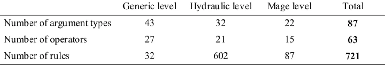
corresponds to an action to be executed by the engine. Operator input/output arguments may have expert-defined types representing elements of descriptive knowledge. Table 3 presents some figures about the current extent of CaRMA-1 knowledge base. Moreover, specific knowledge about two case studies was also implemented in YAKL to form the fact base. It includes descriptions of: (1) the model to be calibrated, namely river topography, geometry of hydraulic structures, and simulation code to be used; (2) events available for calibration, and corresponding measured data; and (3) the modelling objective, namely domain of intended application and performance criteria.
CaRMA-1 architecture, sketched in Figure 4 with UML formalism, includes: the knowledge
base, composed of three levels detailed in Section 3.1; the fact base, with data about the two case studies; and PEGASE+ inference engine, which manipulates objects, plans the calibration subtasks and performs them automatically or interactively by executing rules from the
knowledge base conditioned by information from the fact base. The knowledge level about the use of the MAGE simulation code includes calls to external programs, namely MAGE itself and its pre- and post-processors, to automate every subtask related to numerical simulations: creation of input files from available data, simulation runs, extraction and processing of relevant outputs. Through the user interface and series of prompted closed questions, the user may be requested to provide graphical assessments or supplementary facts during a
calibration session. Moreover, each reasoning step is displayed to make the process completely transparent and to allow the user to assess the consistency of the implemented expert knowledge.
5. Applications
The capability of CaRMA-1 prototype to cope with real-life calibration problems has been verified through its application to two case studies differing from the point of view of the modelling objective, and of the data available to achieve model calibration. Moreover, these cases have been chosen to represent actual common situations in engineering studies where calibration data are often scarce and where the modeller nevertheless has to produce an operational model with the best possible predictive capabilities. The case studies thus illustrate situations where hydraulic expertise is needed to take the best – or the least worst – decisions in the way to perform the calibration according to currently accepted good
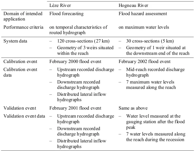
calibration practice. The aim of these case studies is to present how CaRMA-1 can cope with such situations by bringing the user the assistance needed to achieve the calibration task. Characteristics of the case studies, summarized in Table 4, form the fact base of the prototype, from which relevant information is automatically extracted throughout the calibration process. These case studies have also been chosen because of the relatively good representation of the
geometry of the river reaches in terms of the number of cross-sections available.
Unfortunately, the relatively poor number of points in the Hogneau River cross-sections may lead to substantial uncertainties, especially in low water surface profiles.
5.1. River Lèze
The first case study is related to a 25 km reach of the River Lèze, South-West France, between the gauging stations at Lézat (catchment area: 237 km2) and at Labarthe-sur-Lèze (catchment area: 351 km2). The flood selected for calibration is a 5 years return period event for which both recorded hydrographs but also rainfall data were available. The physically-based distributed hydrological code MARINE (Estupina-Borrell et al., 2005) has been used before the calibration study to compute lateral inflows from the intermediate catchment. The following paragraph highlights the main calibration steps of River Lèze model, as supported by CaRMA-1, and specifies the role of the user during each of them.
Data assignment is a completely transparent step: the system picks up the upstream
hydrograph as upstream boundary condition and the rating curve as the downstream boundary condition, and also takes into account the availability of distributed hydrographs for lateral inflows. The remaining data, i.e. discharge downstream hydrograph is selected as a reference. Parameters are then defined interactively: the user has to provide upstream and downstream limits of homogeneous sub-reaches, defined from the point of view of flow resistance. A field visit led to define 8 homogeneous sub-reaches, and thus 8 pairs of resistance coefficients. After choosing between the two methods for initializing resistance parameters (see
Section 3.3), the user is invited to answer a series of questions to describe all sub-reaches. The system can then initialize the parameters thanks to rules like the third one in Table 2, and run
a simulation. MAGE post-processor is then used to display recorded and computed hydrograph at Labarthe. As performance criteria is based on the reproduction of the temporal
characteristics of the routed hydrograph (see Table 4), the system asks the user to describe qualitatively the temporal shift between the two hydrographs. An adjustment step in term of inverse values of Manning's n is then adopted by the system on the basis of answers provided, and applied to adjust all resistance coefficients. The adjustment procedure has been repeated twice for this case study before the temporal adequacy was considered visually satisfactory by the user. Finally, the system asks the user to provide an overall assessment for the calibrated model, which is prompted together with the modelling objective and data used for calibration, in order to summarize model performance derived from the calibration process.
Outputs from the calibrated model are shown in Figure 5 together with calibration data. This representation highlights the fact that no information about the flood is known within the modelled reach and that the calibration can in this case only rely on external data as defined by Bates et al. (1998). Moreover, it is important to note that the only feature which can be assessed in this case is the temporal agreement between the discharge hydrographs, as the reference one is derived from the rating curve used as the downstream boundary condition. The rising part of the recorded downstream hydrograph is well reproduced, which is the most important feature for flood forecasting. On the other hand, the calibrated model overestimates the maximum flood discharge and predicts a double peak hydrograph. These characteristics come from the pattern of lateral inflows simulated by the rainfall-runoff model, and no attempt to reduce these discrepancies has been done – and should be done – during the calibration of the hydraulic model.
Model validation is a complementary task for a global model evaluation (see Figure 1) and is out of the scope of this study. Nevertheless, preliminary tests have been conducted to assess quantitatively the performance of the calibrated model on an independent event. It has been used to simulate a flood recorded in January 2001 which reached a 79 m3/s peak flow. Despite discrepancies in volume due to the hydrological model, the average time shift between the two rising limbs has been found to be +45 minutes for an approximate travel time of 2 hours and 45 minutes. For comparison, the same criterion was equal to -30 minutes for the
calibration event, for a travel time of 4 hours. The model performance thus seems to be roughly adequate for flood forecasting purposes, but could be clearly improved thanks to an iterative or simultaneous calibration with the associated hydrological model.
5.2. River Hogneau
The second case study refers to a 5 km reach of the River Hogneau, located near the border between France and Belgium. A detailed description of this reach can be found elsewhere (Vidal et al., 2004). The return period of the flood selected for this calibration test was estimated to 50 years, which makes this event suitable for a flood hazard assessment study. Moreover, data measured at several locations along the reach make possible to perform a calibration on internal data.
Parameter definition and initialisation are performed as for the River Lèze case study. The Hogneau river reach was divided in 4 homogeneous sub-reaches, and thus led to define 4 pairs of resistance parameters. The system automatically selects measured maximum water levels as reference data, but input data assignment has to be performed interactively due to the lack of obvious boundary conditions. Thus, the system first makes use of data about the
existing weir located at the downstream end of the reach to develop an appropriate critical downstream boundary condition. The system then takes the most upstream recorded hydrograph and uses it as upstream boundary condition to perform some preliminary simulations. The computed and recorded hydrographs at the gauging station are then
displayed and the user is asked to assess the temporal lag. This approach, with all its caveats, is the only solution to model this event on the basis of the available data. The system then shifts the recorded hydrograph back with the given lag to build the final upstream condition, performs a new simulation and displays once again the recorded and computed hydrograph to make the user confirm the agreement. It has been verified that the hydrograph shape is well preserved in this particular case, thanks to the absence of tributaries and to high embankments on both sides of the river (see Vidal et al., 2004). The envelop water surface profile is then displayed together with measured water levels, and questions about possible local
discrepancies within each sub-reach are prompted on the screen. Qualitative answers allow the system to adjust sequentially (in the direction imposed by the subcritical flow), and within their initial physical ranges, the values of the most appropriate parameters: weir discharge coefficient, channel and floodplain resistance coefficients. Once a satisfactory agreement is reached, the system displays the summary of the calibration process.
Outputs from the River Hogneau calibrated model are shown in Figure 6 together with calibration data. The average difference between measured and computed maximum water levels, obtained after a dozen of simulations, was 11.3 cm, which is an acceptable error for flood mapping. For comparison, an optimisation code based on the simulated annealing approach (Kirkpatrick et al., 1983) was run with the same data and found a global optimum parameter set giving an average error of about 9 cm, after several thousands of simulations.
Preliminary validation tests have been performed by comparing the results with independent data from the same event. The average difference between computed and measured water levels during flood recession was found equal to 22.8 cm and the difference between computed and measured water levels at the gauging station just after the flood peak was 12 cm. The discrepancy detected for the low water levels are considered to be resulting from the relatively poor number of points defining each cross-section, but also from changes in the longitudinal bed profile since the available topographical survey. Indeed, the discrepancies are mainly located in a very steep and mobile part of the river reach, located immediately after concrete embankments.
5.3. Discussion
Throughout the successful application to two different case studies, the prototype knowledge-based calibration support system has proved operational and results on these rather extreme cases are encouraging. Further information about the case studies and the detailed calibration sessions with CaRMA-1 can be found elsewhere (Vidal, 2005). CaRMA-1 can deal with several calibration features commonly encountered in actual engineering studies, and provides effective support to any modeller, experienced or not, during the calibration task. It has to be emphasized that no prior specific knowledge about river model calibration or about the use of MAGE is required at all to perform a calibration with CaRMA-1. The expertise required is in fact limited to basic hydraulic knowledge to supply the system with site-specific data and to assess agreements between graphical curves.
Among the 25 generic calibration subtasks identified, 18 are performed automatically on the basis of the hydraulic expert knowledge implemented (see Table 1). Additionally, as
mentioned before, the initialisation of a distributed parameter and the comparison between
reference and prediction require the intervention of the user respectively to describe each homogeneous sub-reach and to assess graphical discrepancies. However, both these subtasks are strictly supervised through the use of closed questions.
Knowledge specific to the hydraulic domain is yet to be implemented for 5 subtasks: first, both case studies chosen to conduct the first tests include only one calibration event, and consequently selection of an event, compilation of comparisons from different events, and
model performance description subtasks are reduced to their simplest expression. Model performance description thus currently simply reflects the reproduction of the single calibration event. As the robustness of calibration parameters can only be assessed through the use of several flood calibration events, corresponding hydraulic knowledge will be needed to face this higher level of situations. Second, selection of a type of distributed parameters is not relevant in 1D river hydraulics – where flow resistance coefficients are the only
distributed parameters –, on the contrary to other water-related domains like distributed hydrological modelling. Finally, definition of homogeneous zones is currently performed entirely in an interactive way and homogeneous sub-reaches are defined by their upstream and downstream limits. Some kind of support might be provided in the future on the basis of an analysis of longitudinal changes in bed topography. More generally, CaRMA-1 features could be incorporated within an existing modelling environment for MAGE, thus allowing the user to perform the computer-aided calibration task with the same interface as other parts of the modelling process.
The knowledge base currently includes mainly generic and hydraulic knowledge for which a consensus has emerged through the last decades of numerical modelling. Any new reasoning
knowledge likely to extend the range of applications of the prototype may easily be added to the knowledge base by adding new concepts (objects) or sub-tasks, or by writing new rules as the ones shown in Table 2. The system could thus help end-users to solve calibration cases requiring different pieces of empirically-derived reasoning knowledge.
Moreover, some prospects of enhancement of CaRMA-1 have been explored to automate currently interactive parts of the calibration process, and thus free the user from intermediate graphical assessments. Preliminary experiments with a symbolic curve evaluation module have for example been conducted to mimic the way an expert visually identifies discrepancies between reference data and a single model prediction (Vidal and Moisan, 2006). This
approach is based on fuzzy qualitative descriptions of segments, peaks, and slope breaks of a computed curve, and of deviations from a set of measured points. Such a module would thus allow the knowledge-based system to simulate multi-objective criteria used by experts during visual assessment.
6. Conclusions
Assessing the credibility of a simulation is a fundamental issue in modern environmental science (Anderson and Bates, 2001). Good practice is thus required at all stages in the development and evaluation of a numerical model (Jakeman et al., 2006), and the predictive ability of a model, assessed through model validation, depends largely on the way the model calibration task is performed. This study focuses on the issue of model calibration in the particular domain of 1D river hydraulics and delineates a prototype knowledge-based system to help a modeller achieving this task in accordance with good calibration practice.
The knowledge base constituting the core of CaRMA-1 has been built upon a review of guidelines extracted from both the literature and interviews with expert modellers. Performing a calibration with the help of this decision support system consequently assures that the process is both reliable and reproducible. It contributes for example to avoid some “bad” practices common in engineering studies: the definition of resistance parameters based on the identification of homogeneous sub-reaches tends to prevent overparametrization of the model (or parameterization dependent on the available calibration data), and the adjustment of parameter values within physical ranges prevents improper and unrealistic forcing of resistance coefficients. Such practice usually compensates for unknown information or poor geometry data on the reach studied, and often stem from the priority given by clients to model accuracy. The approach undertaken in this study clearly favours model effectiveness so that calibration increases the predictive capacity of the model, which is precisely the ultimate purpose of this task. The two case studies illustrate the ability of CaRMA-1 to mimic the way an expert would tackle particular calibration cases, and to get the most reasonable calibrated model considering the data available.
The development of CaRMA-1 opens many prospects for knowledge-based calibration support. Indeed, the architecture of the knowledge base (see Figure 2) has been especially designed for the reuse of its independent levels. Significant parts of the knowledge formalized may thus be reused to build new systems supporting the calibration of models based on different simulation codes, or even models from other domains, like physics-based rainfall-runoff models. Furthermore, the River Lèze case study raised the need for a combined calibration of rainfall-runoff and hydraulic models, which may be undertaken by a similar knowledge-based approach. More generally, knowledge-based decision support systems may
prove well suited in the context of Integrated Assessment and Modelling (IAM) for environmental problems, as described by Parker et al. (2002).
7. Acknowledgements
This work was partially supported by the RIO2 (“Risques InOndations”) program of the French Ministry in charge of the environment (grant n° 01008), and by the ECCO
(“ECosphère COntinentale : processus et modélisation”) program of the French Department in charge of Research. The authors are grateful to Marie-Madeleine Maubourguet for provision of MARINE outputs and would like to thank three anonymous reviewers for helpful comments on earlier versions of this manuscript.
Figure 1. Elements of a modelling terminology, modified after Refsgaard and Henriksen (2004). The outer plain arrows refer to the procedures which evaluate the credibility of the processes described by inner dashed arrows. Dotted arrows show the use of measured data from the physical system considered.
Figure 2. Knowledge levels in model calibration.
Figure 3. A formalisation of model calibration process – UML activity diagram. The seven calibration steps are shown as rounded rectangles, and items used and produced by each calibration step are shown by rectangles with underlined content. Collections of items are represented as two shifted rectangles. Solid and dashed arrows denote object flows, decisions are represented by diamonds, and thick bars show synchronisation states.
Figure 4. Architecture of CaRMA-1 – UML deployment diagram. Arrows represent data flow. See text for details.
Figure 5. Representation of the February 2000 Lèze flood. The shaded 3-D surface corresponds to the outputs of the numerical model, stars are recorded upstream flows, and plus signs are recorded downstream flows.
Figure 6. Representation of the February 2002 Hogneau flood. The shaded 3-D surface corresponds to the outputs of the numerical model, and lines represent measured maximum water levels. Line extents show the temporal uncertainty (here taken as one day) about the maximum level recorded during the flood.
Table 1: List of generic subtasks implemented in CaRMA-1. Fist level subtasks correspond to calibration step showed in Figure 3. Depending on the actual calibration case, the internal structure of each first-level subtask may not include some second-level subtasks and include loops over some others (e.g., Initialisation of a distributed parameter). A black filled circle denotes a fully operational implementation, whereas a white circle denotes a default implementation.
Operating Mode First level Second level
Automatic Interactive
Selection of an event ●
Selection of event input data ●
Data assignment
Selection of event reference data ●
Selection of a structure ●
Definition of a structure parameter ●
Definition of homogeneous zones ○
Selection of an homogeneous zone ●
Parameter definition
Definition of a distributed parameter ● Initialisation of a structure parameter ● Parameter
initialisation
Initialisation of a distributed parameter ●
Preprocessing ●
Execution of the simulation code ●
Simulation run
Postprocessing ●
Selection of reference data ●
Selection of a prediction ●
Comparison between reference and prediction ●
Output comparison
Compilation of comparisons from different events ○
Selection of a structure parameter ●
Adjustment of structure parameter ●
Selection of a distributed parameter ●
Adjustment of a distributed parameter ● Selection of a class of distributed parameters ○
Parameter adjustment
Adjustment of a class of distributed parameters ● Model
performance description
Table 2. Example of semi-formalized hydraulic rules attached to different second-level subtasks. The “.” notation is for using attributes of a class, as in standard object-oriented languages.
Subtask Rule example
Selection of input data If DischargeHydrograph.location = Reach.upstreamEnd Then DischargeHydrograph.useForUpstreamBoudaryCondition = ‘yes’ Definition of a
structure parameter
If Weir.shape ≠ ‘ideal’ Then DischargeCoefficient.isParameter = ‘yes’
Initialisation of a distributed parameter
If Reach.nature = ‘natural’ and Reach.size = ‘minorStream’ and Reach.location = ‘on plain’ and Reach.description = ‘clean, straight, full stage, no rifts or deep pools’ Then n.min = 0.025 and n.mean = 0.030 and n.max = 0.033
Selection of a prediction
If EventReferenceData.type = ‘floodmarks’ and EventPrediction.type = ‘EnvelopWaterProfile’ Then EventPrediction.useForComparison = ‘yes’
Adjustment of a distributed parameter
If EventReferenceData.type = ‘WaterLevel’ and EventPrediction.discrepancy = ‘tooHigh’ Then ResistanceCoefficient.adjustment = ‘increase’
Table 3. Figures about the current state of CaRMA-1 knowledge base.
Generic level Hydraulic level Mage level Total
Number of argument types 43 32 22 87
Number of operators 27 21 15 63
Table 4. Characteristics of the case studies.
Lèze River Hogneau River
Domain of intended
application Flood forecasting Flood hazard assessment
Performance criteria on temporal characteristics of
routed hydrograph on maximum water levels System data – 120 cross-sections (27 km)
– Geometry of 3 weirs situated within the reach
– 30 cross-sections (5 km) – Geometry of 1 weir situated at
the downstream end of the reach Calibration event February 2000 flood event February 2002 flood event
Calibration event data
– Upstream recorded discharge hydrograph
– Downstream recorded discharge hydrograph – Distributed lateral inflow
hydrographs
– Mid-reach recorded discharge hydrograph
– 7 maximum water levels measured along the reach
Validation event February 2001 flood event Same as above Validation event data – Upstream recorded discharge
hydrograph
– Downstream recorded discharge hydrograph – Distributed lateral inflow
hydrographs
– Water level measured at the gauging station after the flood peak
– 7 water levels measured along the reach during the recession
8. References
Abbott, M.B., 1991. Hydroinformatics – Information Technology and the Aquatic Environment. Avebury Technical: Alderschot, U.K.
Abbott, M.B., 1994. Hydroinformatics: a Copernican revolution in hydraulics. Journal of Hydraulic Research 32 (extra issue) 3-14.
Abbott, M.B., Babovic, V.M., Cunge, J.A., 2003. Reply to comments on "Towards the hydraulics of the hydroinformatics era". Journal of Hydraulic Research 41 (3) 333-336.
Anastasiadou-Partheniou, L., Samuels, P.G., 1998. Automatic calibration of computational river models. Proceedings of the Institution of Civil Engineers-Water Maritime and Energy 130 (3) 154-162.
Anderson, M.G., Bates, P.D., 2001. Model Validation: Perspectives in Hydrological Science. Wiley: Chichester, U.K.
Anderson, M.P., Woessner, W.W., 1992. The role of the postaudit in model validation. Advances in Water Resources 15 (3) 167-173.
Arcement, G.J., Schneider, V.R., 1984. Guide for selecting Manning's roughness coefficients for natural channels and flood plains. Final Report FHWA-TS-84-204. Federal Highway Administration.
Barnes, H.H., 1967. Roughness characteristics of natural channels. Water Supply Report 1849. US Geological Survey.
Bates, P.D., Anderson, M.G., 2001. Validation of hydraulic models. In: Anderson, M.G., Bates, P.D., (Eds.), Model Validation: Perspectives in Hydrological Science. Wiley: Chichester, U.K.
Bates, P.D., Stewart, M.D., Siggers, G.B., Smith, C.N., Hervouet, J.-M., Sellin, R.H.J., 1998. Internal and external validation of a two-dimensional finite element code for river flood simulations. Proceedings of the Institution of Civil Engineers-Water Maritime and Energy 130 (3) 127-141.
Beven, K.J., Binley, A.M., 1992. The future of distributed models – Model calibration and uncertainty Prediction. Hydrological Processes 6 (3) 279-298.
Brunner, G.W., 2002. Hec-Ras, River Analysis System – User's manual. Computer Program Documentation CPD-68. US Army Corps of Engineers, Institute for Water Resources, Hydrologic Engineering Center.
Castaings, W., Dartus, D., Honnorat, M., Loukili, Y., Le Dimet, F.-X., Monnier, J., 2005. Automatic differentiation: a tool for variational data assimilation and adjoint sensitivity analysis for flood modeling. In: Bücker, H.M., Corliss, G., Hovland, P., Naumann, U., Norris, B., (Eds.), Automatic Differentiation: Applications, Theory, and Tools. Springer: Chicago, Illinois.
Chau, K.W., 2003. Manipulation of numerical coastal flow and water quality models. Environmental Modelling & Software 18 (2) 99-108.
Chau, K.W., Chuntian, C., Li, C.W., 2002. Knowledge management system on flow and water quality modeling. Expert Systems with Applications 22 (4) 321-330. Chow, V.T., 1959. Open-Channel Hydraulics. McGraw-Hill: New York, USA.
Cowan, W.L., 1956. Estimating hydraulic roughness coefficients. Agricultural Engineering 37 (7) 473-475.
Cunge, J.A., 2003. Of data and models. Journal of Hydroinformatics 5 (2) 75-98. Cunge, J.A., Holly , F.M.J., Verwey, A., 1980. Practical aspects of computational river
hydraulics. Pitman: London, U.K.
Dai, J.J., Lorenzato, S., Rocke, D.M., 2004. A knowledge-based model of watershed assessment for sediment. Environmental Modelling & Software 19 (4) 423-433. Dalrymple, T., Benson, M.A., 1967. Measurement of peak discharge by the slope-area
method. Techniques of Water-Resources Investigations Report, Chapter A2. US Government Printing Office.
Defra/EnvironmentAgency, 2003. Reducing uncertainty in river flood conveyance -- Review of methods for estimating conveyance. Interim Report 2 W5A – 057.
Defra/Environment Agency.
Dhondia, J.F., 2004. Good modelling practice using Sobek - An integrated hydraulics
modelling package. In: Liong, S.Y., Phoon, K.-K., Babovic, V.M., (Eds.), Proceedings of the Sixth International Conference on Hydroinformatics. World Scientific
Publishing Company: Singapore.
Ding, Y., Jia, Y., Wang, S.S.Y., 2004. Identification of Manning's roughness coefficients in shallow water flows. Journal of Hydraulic Engineering 130 (6) 501-510.
Ermine, J.-L., Chaillot, M., Bigeon, P., Charreton, B., Malavielle, D., 1996. MKSM, a method for knowledge management. In: Schreinemakers, J.F., (Eds.), Knowledge
Management: Organization, Competence and Methodology – Proceedings of the fourth International ISMICK Symposium. Ergon Verlag: Rotterdam, The Netherlands. Estupina-Borrell, V., Chorda, J., Dartus, D., 2005. Flash-flood anticipation. Comptes-rendus
Géosciences 337 (13) 1109-1119.
Fisher, K.R., Dawson, H., 2003. Reducing uncertainty in river flood conveyance - Roughness review. DEFRA / Environment Agency, Project W5A – 57.
French, R.H., 1994. Open-Channel Hydraulics. Mc Graw-Hill International Editions. Giraud, F., Faure, J.-B., Zimmer, D., Lefeuvre, J.C., Skaggs, R.W., 1997. Hydrologic
modeling of a complex wetland. Journal of Irrigation and Drainage Engineering 123 (5) 344-353.
Guinot, V., Gourbesville, P., 2003. Calibration of physically based models: back to basics? Journal of Hydroinformatics 5 (4) 233-244.
Hicks, D.M., Mason, P.D., 1998. Roughness Characteristics of New Zealand Rivers. National Institute of Water and Atmospheric Research – Water Resources Publications, LLC: Englewood, Colorado.
Hill, M.C., 1998. Methods and guidelines for effective model calibration. Water Resources Investigations Report 98-405. US Geological Survey.
Jakeman, A.J., Letcher, R.A., Norton, J.P., 2006. Ten iterative steps in development and evaluation of environmental models. Environmental Modelling & Software 21 (5) 602-614.
Jarrett, R.D., Petsch, H.E., 1985. Computer program Ncalc user's manual - Verification of Manning's roughness coefficient in channels, US Geological Survey: 27.
Kirkpatrick, S., Gelatt, C.D.Jr., Vecchi, M.P., 1983. Optimization by simulated annealing. Science 220 (4598) 671-683.
Klemeš, V., 1986. Operational testing of hydrological simulation models. Hydrological Sciences Journal 31 (1) 13-24.
Madsen, H., 2003. Parameter Estimation in Distributed Hydrological Catchment Modelling Using Automatic Calibration with Multiple Objectives. Advances in Water Resources 26 (2) 205-216.
Manning, R., 1891. On the flow of water in open channels and pipes. Transactions of the Institution of Civil Engineers of Ireland 20 161-207.
Marsh, S.B., Johnson, G.P., Holmes, R.H., 2004. Data base and computational tools to aid in determination of roughness coefficients of streams. Water Resources Investigation Report, in Progress US Geological Survey.
McGahey, C., Samuels, P.G., 2004. River roughness - The integration of diverse knowledge. In: Greco, M., Carravetta, A., Della Morte, R., (Eds.), River Flow 2004 – Proceedings of the Second International Conference on Fluvial Hydraulics. Balkema: Napoli, Italy. McIntosh, B.S., 2003. Qualitative modelling with imprecise ecological knowledge: a
framework for simulation. Environmental Modelling & Software 18 (4) 295-307. Moisan, S., 2002. Knowledge representation for program reuse. In: van Harmelen, F., (Eds.),
Proceedings of the 15th European Conference on Artificial Intelligence, ECAI-2002. IOS Press: Lyon, France.
Moore, C., Doherty, J., 2005. Role of the calibration process in reducing model predictive error. Water Resources Research 41 (W05020).
Muzy, A., Innocenti, E., Aïello, A., Santucci, J.-F., Santoni, P.-A., Hill, D.R.C., 2005. Modelling and simulation of ecological propagation processes: application to fire spread. Environmental Modelling & Software 20 (7) 827-842.
OMG, 2003. Unified Modeling Language (UML) specification – Version 1.5. Group, O.M. Needham, Massachussetts.
Papajorgji, P., Shatar, T.M., 2004. Using the Unified Modeling Language to develop soil water-balance and irrigation-scheduling models. Environmental Modelling & Software 19 (5) 451-459.
Parker, P., Letcher, R., Jakeman, A., Beck, M.B., Harris, G., Argent, R.M., Hare, M., Pahl-Wostl, C., Voinov, A., Janssen, M., 2002. Progress in integrated assessment and modelling. Environmental Modelling & Software 17 (3) 209-217.
Picard, S., Ermine, J.-L., Scheurer, B., 1999. Knowledge management for large scientific software. (Eds.), Proceedings of the second International Conference on the Practical Application of Knowledge Management – PAKeM'99. The Practical Application Company: London, U.K.
Refsgaard, J.C., 1996. Terminology, modelling protocol and classification of hydrological model codes. In: Abbott, M.B., Refsgaard, J.C., (Eds.), Distributed Hydrological Modelling. Kluwer: Dordrecht, The Netherlands.
Refsgaard, J.C., Henriksen, H.J., 2004. Modelling guidelines - Terminology and guiding principles. Advances in Water Resources 27 (1) 71-82.
Refsgaard, J.C., Henriksen, H.J., Harrar, W.G., Scholten, H., Kassahun, A., 2005. Quality Assurance in model based water management – Review of existing practice and outline of new approaches. Environmental Modelling & Software 20 (10) 1201-1215. Romanowicz, R.J., Beven, K.J., 2003. Estimation of flood inundation probabilities as
conditioned on event inundation maps. Water Resources Research 39 (3) 1073. Rouse, H., 1965. Critical analysis of open-channel resistance. Journal of the Hydraulics
Division 91 (4) 1-25.
Schlesinger, S., Crosbie, R.E., Gagné, R.E., Innis, G.S., Lalwani, C.S., Loch, J., Sylvester, R.J., Wright, R.D., Kheir, N., Bartos, D., 1979. Terminology for model credibility. Simulation 32 (3) 103-104.
Seed, D.J., Samuels, P.G., Ramsbottom, D.M., 1993. Quality Assurance in computational river modelling. First Interim Report SR374. HR Wallingford.
Spear, R.C., 1997. Large simulation models: calibration, uniqueness and goodness of fit. Environmental Modelling & Software 12 (2-3) 219-228.
Thonnat, M., Moisan, S., Crubézy, M., 1999. Experience in integrating image processing programs. In: Christensen, H.I., (Eds.), Computer Vision Systems - Proceedings of the first International conference, ICVS'99. Springer: Las Palmas, Spain.
van Waveren, R.H., Groot, S., Scholten, H., van Geer, F.C., Wösten, J.H.M., Koeze, R.D., Noort, J.J., 1999. Good modelling practice handbook. STOWA Report 99-05. RWS-RIZA.
Vidal, J.-P., 2005. Assistance au calage de modèles numériques en hydraulique fluviale – Apports de l'intelligence artificielle (Computer-aided model calibration in river hydraulics – Contributions from artificial intelligence, in French). PhD thesis: Institut National Polytechnique de Toulouse (available from
http://www.lyon.cemagref.fr/doc/these/vidal/).
Vidal, J.-P., Faure, J.-B., Moisan, S., Dartus, D., 2004. Decision support system for
calibration of 1-D river models. In: Liong, S.Y., Phoon, K.-K., Babovic, V.M., (Eds.), Proceedings of the 6th International Conference on Hydroinformatics. World
Scientific Publishing: Singapore.
Vidal, J.-P., Moisan, S., 2006. Fuzzy knowledge-based curve evaluation for 1-D river model calibration. In: Gourbesville, P., Cunge, J.A., Guinot, V., Liong, S.-Y., (Eds.), Hydroinformatics 2006 – Proceedings of the 7th International Conference on Hydroinformatics. Research Publishing: Chennai, India.
Vidal, J.-P., Moisan, S., Faure, J.-B., 2003. Knowledge-based hydraulic model calibration. Lecture Notes in Computer Science 2773 676-683.
Vidal, J.-P., Moisan, S., Faure, J.-B., Dartus, D., 2005. Towards a reasoned 1-D river model calibration. Journal of Hydroinformatics 7 (2) 91-104.
Yang, L., Lin, B., Kashefipour, S.M., Falconer, R.A., 2002. Integration of a 1-D river model with object-oriented methodology. Environmental Modelling & Software 17 (8) 693-701.
Yen, B.C., 1999. Discussion about “Identification problem of open-channel friction parameters”. Journal of Hydraulic Engineering 125 (5) 552-553.
Yen, B.C., 2002. Open channel flow resistance. Journal of Hydraulic Engineering 128 (1) 20-39.
Physical
System
Conceptual
Model
Numerical
Model
Model
Validation
Predictive
Simulation
Analysis
Programming
Theory
Confirmation
Code
Verification
Simulation
Code
Model
Set-up
Model
Calibration
Data
Measurements
Physical
System
Conceptual
Model
Numerical
Model
Model
Validation
Predictive
Simulation
Analysis
Programming
Theory
Confirmation
Code
Verification
Simulation
Code
Model
Set-up
Model
Calibration
Data
Measurements
Figure 1ModelCalibration SimulationRun OutputComparison ModelPerformanceDescription :EventInputDataSet :EventPrediction
[best possible agreement] :EventReferenceDataSet :EventPrediction :EventData [calibrated] :NumericalModel :EventData :DomainOfIntendedApplication ParameterDefinition [uncalibrated] :NumericalModel :EventReferenceData :EventReferenceData DataAssignment :PerformanceCriteria ParameterAdjustment ParameterInitialisation
[with defined parameters] :NumericalModel
[with attributed parameter values] :NumericalModel [perfectible agreement] :EventReferenceDataSet [perfectible agreement] :EventReferenceDataSet [tested] :NumericalModel :DomainOfApplicability [else] [perfectible agreement]
[parameter definition ok]
[else]
Knowledge about the system studied
and its numerical model
Knowledge about
the use of the simulation code
Domain knowledge
Generic knowledge about model calibration
MAGE CaRMA-1 MagePreprocessors MagePostprocessors UserInterface KnowledgeBase FactBase PEGASE+ GenericKnowledge HydraulicKnowledge MageKnowledge LèzeFacts HogneauFacts Figure 4