An analysis of Atlantic water in the Arctic Ocean using the Arctic Subpolar gyre state estimate and observations

(1)

An Analysis of Atlantic Water in the Arctic Ocean Using the

Arctic Subpolar Gyre State Estimate and Observations

by

Lieutenant Commander Jeffrey Scott Grabon, United States Navy

B.S., The Pennsylvania State University (2007)

M.S., The Pennsylvania State University (2009)

Submitted to the Department of Earth, Atmospheric and Planetary Sciences in partial fulfillment of the requirements for the degree of

Master of Science in Physical Oceanography at the

MASSACHUSETTS INSTITUTE OF TECHNOLOGY and the

WOODS HOLE OCEANOGRAPHIC INSTITUTION September 2020

c

The author hereby grants to MIT and WHOI permission to reproduce and to distribute publicly paper and electronic copies of this thesis document in whole or in

part in any medium now known or hereafter created.

Author . . . . Department of Earth, Atmospheric and Planetary Sciences

Massachusetts Institute of Technology & Woods Hole Oceanographic Institution August 7, 2020 Certified by. . . . John Toole Senior Scientist Woods Hole Oceanographic Institution Thesis Supervisor Accepted by . . . .

Glenn R. Flierl Chairman, Joint Committee for Physical Oceanography Massachusetts Institute of Technology

(2)

(3)

An Analysis of Atlantic Water in the Arctic Ocean Using the Arctic Subpolar Gyre State Estimate and Observations

by

Lieutenant Commander Jeffrey Scott Grabon, United States Navy

Submitted to the Department of Earth, Atmospheric and Planetary Sciences Massachusetts Institute of Technology

& Woods Hole Oceanographic Institution on August 7, 2020, in partial fulfillment of the

requirements for the degree of

Master of Science in Physical Oceanography

Abstract

The Atlantic Water (AW) Layer in the Arctic Subpolar gyre sTate Estimate (ASTE), a re-gional, medium-resolution coupled ocean-sea ice state estimate, is analyzed for the first time using bounding isopycnals. A surge of AW, marked by rapid increases in mean AW Layer potential temperature and AW Layer thickness, begins two years into the state estimate (2004) and traverses the Arctic Ocean along boundary current pathways at approximately 2 cm/s. The surge also alters AW flow direction and speed including a significant reversal in flow direction along the Lomonosov Ridge. The surge results in a new quasi-steady AW flow from 2010 through the end of the state estimate period in 2017. The time-mean AW circulation during this time period indicates a significant amount of AW spreads over the Lomonosov Ridge rather than directly returning along the ridge to Fram Strait. A three-layer depiction of ASTE’s overturning circulation within the AO indicates AW is converted to colder, fresher Surface Layer water at a faster rate than is transformed to Bottom Water (1.2 Sv vs. 0.4 Sv). Observed AW properties compared to ASTE output indicate increas-ing misfit durincreas-ing the simulated period with ASTE’s AW Layer generally beincreas-ing warmer and thicker than in observations.

Thesis Supervisor: John Toole Title: Senior Scientist

(4)

(5)

Acknowledgments

This research was funded via the United States Navy’s Civilian Institution Program with the MIT/WHOI Joint Program (JP).

The thesis supervisor’s participation in this project was supported by National Science Foundation-Grant #PLR-1603660 and by Office of Naval Research-Grant #N000141612381. This project, specifically ASTE developed by Dr. An T. Nguyen, is also supported by National Science Foundation-Grant #PLR-1603903.

The Ice-Tethered Profiler data were collected and made available by the Ice-Tethered Profiler Program (Toole et al., 2011; Krishfield et al., 2008) based at the Woods Hole Oceanographic Institution (http://www.whoi.edu/itp).

Some CTDs used in this research were collected and made available by the Beaufort Gyre Exploration Program based at the Woods Hole Oceanographic Institution (https:// www.whoi.edu/beaufortgyre) in collaboration with researchers from Fisheries and Oceans Canada at the Institute of Ocean Sciences.

Thank you Dr. An T. Nguyen, Oden Institute for Computational Engineering and Sciences, University of Texas, for providing the ASTE output for this project as well as quick, thorough responses to my inquiries.

Thank you Dr. Christopher Piecuch, Assistant Scientist at the Woods Hole Oceano-graphic Institution, for his guidance explaining the contents of various ASTE files and step-ping through how to apply them to the problem at hand. His in-depth discussions provided a framework to tackle several tasks.

Thank you Richard A. Krishfield, Senior Research Specialist at Woods Holde Oceano-graphic Institution, for his help obtaining observations to conduct this analysis.

I especially want to express my gratitude to my advisor, Dr. John Toole, for providing his support and guidance over the last two years. When I arrived at WHOI, I searched for a faculty member with a project related to the Arctic Ocean. He proposed an analysis of the Atlantic Water Layer in ASTE. Not really knowing what I was agreeing to, I decided this would be a terrific opportunity. In retrospect, it truly was! I was handed an external hard drive full of output and off I went. Ten years removed from academia and eight years into my naval career, my computer programming skills were quite rusty and severely lacking. I had no idea what an isopycnal was and an environment stratified by salinity was especially

(6)

foreign. Clearly, I needed an advisor with patience who was willing to build an oceanographer from the bottom up. Perhaps he had no idea what he was getting himself into either! He provided the right amount of direction without micromanaging and was understanding when I needed more time to accomplish a task. I think it is an especially noteworthy achievement that we were able to complete this project with only virtual meetings during the final six months as a result of the pandemic (COVID-19).

This thesis is only a portion of the academic work required for graduation. My classmates and friends were an integral part of the experience as we commiserated through coursework together. Thank you Stephan Gallagher, Praneeth Gurumurthy, Hanyuan Liu, Martin Velez Pardo, and Casey Densmore who were my office mates on the sixteenth floor of MIT’s Green Building. I especially want to express my appreciation to Casey who was many times my one-stop resource for MATLAB and coursework help. I would also like to thank fellow shipmates Brendan O’Neill, Chris Dolan, Mike Humara, John Li, and Kyle Kausch. My student mentor, Astrid Pacini, was also a helpful resource for navigating this program.

Finally, I’d like to thank my family. As a native New Englander, I was able to spend time with family I used to only have the opportunity to see a couple weeks a year. I especially want to thank my wife, Lindsey Grabon, and daughter, Norah Grabon, for their love and support during this tour. This adventure began between deployments when Lindsey and I flew to Osaka and Tokyo so I could take the GRE. It was not administered electronically on Okinawa and was required for the MIT/WHOI JP application. After being accepted, we arrived in Massachusetts with Lindsey eight months pregnant. There was a quick turn around to establish a home but we were fully prepared to welcome Norah to the world. This tour ended with all three of us at home together for the final six months due to the COVID-19 pandemic. While it introduced many new challenges, it provided memories I’ll cherish for a lifetime.

(7)

List of Figures

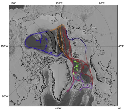
1-1 A simplified, time-mean depiction of the AW circulation in the Nordic Seas and Arctic Ocean inferred from sparse hydrographic observations. AW enters the AO through Fram Strait and the Barents Sea. The two branches meet in the St. Anna Trench as they circulate cyclonically in the AO. Bifurcations of the AW circumpolar boundary current occur at each ridge. Image from Mauritzen et al., 2013 [1] which was adapted from Rudels et al., 2012 [2]. . . 21

2-1 Major geographic and bathymetric features in the AO, Nordic Seas and North Atlantic. Image is from Mauritzen et al., 2013 [1] which was adapted from Rudels et al., 2012 [2]. . . 29

(10)

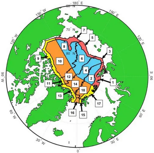
2-2 The AO partitioning scheme developed to examine AW properties. On the Eurasian side of each basin, circumpolar subbasins are colored red and mid subbasins are blue. On the North American side, circumpolar subbasins are colored yellow and mid subbasin are orange. Numbered subbasins are as follows: 1. Eurasian Circumpolar Nansen Basin (ECNB), 2. Eurasian Mid Nansen Basin (EMNB), 3. Eurasian Circumpolar Amundsen Basin (ECAB), 4. Eurasian Mid Amundsen Basin (EMAB), 5. Eurasian Circum-polar Makarov Basin (ECMB), 6. Eurasian Mid Makarav Basin (EMMB), 7. Eurasian Circumpolar Canada Basin (ECCB), 8. Eurasian Mid Canada Basin (EMCB), 9. North American Circumpolar Canada Basin (NCCB), 10. North American Mid Canada Basin (NMCB), 11. North American Circumpolar Makarov Basin (NCMB), 12. North American Mid Makarov Basin (NMMB), 13. North American Greenland Circumpolar Amundsen Basin (NGCAB), 14. North American Poleward Mid Amundsen Basin (NPMAB), 15. North American Svalbard Circumpolar Amundsen Basin Svalbard (NSCAB), 16. North American Fram Mid Amundsen Basin (NFMAB), 17. North American Circumpolar Nansen Basin (NCNB), 18. North American Mid Nansen Basin (NMNB). . . 31 2-3 The Lomonosov Boundary Current contour is depicted in red. The contour

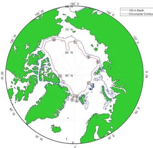
is produced using the circumpolar and mid subbasin boundaries depicted in Figure 2-2 and a 100 km buffer region along the Lomonosov Ridge. Letters mark the beginning and end of the contour as well as subbasin transitions. The blue contour is the 100 m isobath. . . 32 2-4 The Circumpolar Boundary Current contour is depicted in red which follows

the subbasin boundaries depicted in Figure 2-2. Letters mark the beginning and end of the contour as well as subbasin transitions. The blue contour is the 100 m isobath. . . 33 2-5 The AW Layer bounding isopycnals for this study plotted on mean potential

density referenced to 200 dbar versus mean potential temperature referenced to the 0 dbar profiles for the EMNB (green) and NMCB (blue) subbasins with one standard deviation about the mean shaded. Subbasin depictions and acronyms are provided in Figure 2-2. . . 35

(11)

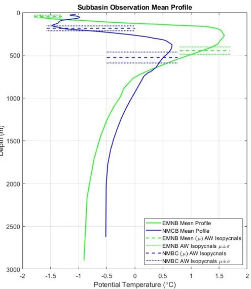
2-6 The mean depth versus potential temperature profiles for the EMNB (green) and NMCB (blue) subbasins. The mean depths (dashed) and standard devi-ation (dotted) of the bounding AW isopycnals are plotted in the same color as their associated subbasin profile with the 1028.2 kg/m3 _{isopycnal located}

higher in the water column than 1028.9 kg/m3_{. . . 36}

2-7 The AW Layer bounding isopycnals for this study plotted against mean pres-sure versus potential density profiles for the EMNB (green) and NMCB (blue) subbasins with one standard deviation about the mean shaded. . . 37 2-8 The ASTE grid x- and y-coordinates relative to major geographic features

overlaid on bathymetry. Latitude lines are drawn every 5∘ _{and longitude}

every 15∘_{. . . 39}

3-1 Mean AW Layer (1028.2 kg/m3 _{- 1028.9 kg/m}3_{) potential temperature, Θ} 𝑎𝑣,

from January 2010 through December 2017 in ASTE. Values are displayed only for those grid cells where both upper and lower bounding isopycnals existed in each monthly mean profile. . . 44 3-2 Mean AW Layer (1028.2 kg/m3 _{- 1028.9 kg/m}3_{) thickness from January 2010}

through December 2017 in ASTE. Values are displayed only for those grid cells where both upper and lower bounding isopycnals existed in each monthly mean profile. . . 45 3-3 Mean 1028.2 kg/m3 _{isopycnal depth from January 2010 through December}

2017 in ASTE. Only grid cells where both top and bottom AW bounding isopycnals exist in every monthly mean file are displayed. . . 47 3-4 Mean 1028.9 kg/m3 _{isopycnal depth from January 2010 through December}

2017 in ASTE. Values are displayed only for those grid cells where both upper and lower bounding isopycnals existed in each monthly mean profile. . . 48 3-5 The full (divergent and non-divergent) transport streamfunction for the mean

AW Layer (1028.2 kg/m3_{- 1028.9 kg/m}3_{) from January 2010 through}

Decem-ber 2017 in ASTE output. The contour interval is 0.25 Sv. Bathymetry is indicated with color. . . 50

(12)

3-6 The non-divergent Transport Streamfunction for the mean AW Layer (1028.2 kg/m3_{) - 1028.9 kg/m}3_{) from January 2010 through December 2017 of monthly}

mean ASTE output. The contour interval is 0.25 Sv. . . 51 3-7 Streamlines for the mean AW Layer velocity from January 2010 through

De-cember 2017. . . 52 3-8 The mean overturning circulation for the Surface Layer, AW Layer, and

Bot-tom Layer from January 2010 through December 2017 in ASTE. . . 54 3-9 The average seasonal cycle of volume transport for the AW inflow through

Fram Strait (red, dash-dot), AW outflow through Fram Strait (blue, solid), and AW inflow through the Barents Sea (red, dashed) for each month from January 2010 through December 2017. The locations used to calculate the volume transport are depicted in Figures 3-5 and 3-6. The location used for the Barents Sea inflow is off the coast of Novaya Zemlya. . . 55 3-10 The average speed of the AW Layer for each month along the Lomonosov

Boundary Current contour from 2010-2017. . . 56 3-11 The average AW Layer speed for each month along the Circumpolar Boundary

Current contour from 2010-2017. . . 57 3-12 The average volume transport for the AW inflow through Fram Strait (red,

dash-dot), AW outflow through Fram Strait (blue, solid), and AW inflow through the Barents Sea (red, dashed) for each month of ASTE output. The locations used to calculate the volume transport are depicted in Figures 3-5 and 3-6 with the Barents Sea inflow based on the coordinates off the coast of Novaya Zemlya. . . 58 3-13 The average AW speed along the Lomonosov Boundary Current contour for

each month of ASTE output. . . 59 3-14 The average AW speed along the Circumpolar Boundary Current contour for

each month of ASTE output. . . 60 3-15 Monthly mean AW Layer (1028.2 kg/m3_{) - 1028.9 kg/m}3_{) velocity at four}

year intervals beginning in January 2002 for grid locations where both AW bounding isopycnals exist. Color shading identifies the AW speed while direc-tion is indicated with streamlines. The 500 m bathymetry contour is indicated in blue. . . 62

(13)

3-16 Top: The grid-relative AW Layer velocity angle along the Lomonosov Bound-ary Current contour as a function of time (y-axis) and space (x-axis). The angle definitions are as follows: 0∘ _{is grid-relative East, 90}∘ _{is grid-relative}

North, 180∘ _{or -180}∘ _{is grid-relative West, and -90}∘ _{is grid-relative South.}

Vertical dashed lines show subbasin transitions along the contour with labels on the top x-axis corresponding to the locations on the contour identified in Figure 2-3. Bottom: The AW speed along the contour as a function of time and space. . . 64 3-17 Monthly mean AW Layer potential temperature, Θ𝑎𝑣, at four year intervals

for the duration of the ASTE output. Only ASTE grid locations with both upper and lower AW bounding isopycnals are plotted. . . 66 3-18 Monthly mean AW Layer thickness at four year intervals for the duration of

the ASTE output. Only ASTE grid locations where both upper and lower isopycnals exist are plotted. . . 67 3-19 Monthly mean 1028.2 kg/m3 _{isopycnal depth at four year intervals for the}

duration of the ASTE output. Only ASTE grid locations where both upper and lower isopycnals exist are plotted. . . 69 3-20 Monthly mean 1028.9 kg/m3 _{isopycnal depth at four year intervals for the}

duration of the ASTE output. Only ASTE grid locations where both upper and lower isopycnals exist are plotted. . . 70 3-21 Top: Time versus distance along the Lomonosov Boundary Current contour of

AW Layer potential temperature, Θ𝑎𝑣. Bottom: Time versus distance along

the Circumpolar Boundary Current contour of AW llyer potential tempera-ture, Θ𝑎𝑣. Vertical dashed lines indicate subbasin transition locations with

letters on the top axis corresponding to locations identified in Figures 2-3 and 2-4. The distance along each contour is identified on the bottom axis. . . 72 3-22 Top: Time versus distance along the Lomonosov Boundary Current contour

of AW Layer thickness. Bottom: Time versus distance along the Circumpolar Boundary Current contour of AW Layer thickness. Vertical dashed lines indi-cate subbasin transition locations with letters on the top axis corresponding to locations identified in Figures 2-3 and 2-4. The distance along each contour is identified on the bottom axis. . . 73

(14)

3-23 Top: Time versus distance along the Lomonosov Boundary Current contour of the AW upper boundary, 1028.2 kg/m3_{, depth. Bottom: Time versus distance}

along the Circumpolar Boundary Current contour of the AW upper bound-ary, 1028.2 kg/m3_{, depth. Vertical dashed lines indicate subbasin transition}

locations with letters on the top axis corresponding to locations identified in Figures 2-3 and 2-4. The distance along each contour is identified on the bottom axis. . . 74

3-24 Top: Time versus distance along the Lomonosov Boundary Current contour of the AW lower boundary, 1028.9 kg/m3_{, depth. Bottom: Time versus distance}

along the Circumpolar Boundary Current contour of the AW lower bound-ary, 1028.9 kg/m3_{, depth. Vertical dashed lines indicate subbasin transition}

locations with letters on the top axis corresponding to locations identified in Figures 2-3 and 2-4. The distance along each contour is identified on the bottom axis. . . 75

3-25 Top Left: The difference between the observed (CTD or ITP) AW Θ𝑎𝑣 and

the ASTE AW Θ𝑎𝑣 for the closest grid location to the observation at the

time of each observation in the EMNB subbasin. A 36 month running mean of the differences is plotted in a black dashed line. Top Right: The ASTE AW Θ𝑎𝑣 for the closest grid location to the observation during the month of

the observation. The black dashed line is a 36 month running mean of the ASTE AW Θ𝑎𝑣 values at the nearest grid location to the observation. The

red line is the overall subbasin mean ASTE AW Θ𝑎𝑣 value. Bottom Left: The

observed AW Θ𝑎𝑣 for CTDs (squares) and ITP (circles). The red line is the

overall subbasin mean ASTE AW Θ𝑎𝑣 value. Bottom Right: The number of

(15)

3-26 Top Left: The difference between the observed (CTD or ITP) AW thickness and the ASTE AW thickness for the closest grid location to the observation at the time of each observation in the EMNB subbasin. A 36 month running mean of the differences is plotted in a black dashed line. Top Right: The ASTE AW thickness for the closest grid location to the observation during the month of the observation. The black dashed line is a 36 month running mean of the ASTE AW thickness values at the nearest grid location to the observation. The red line is the overall subbasin mean ASTE AW thickness value. Bottom Left: The observed AW thickness for CTDs (squares) and ITP (circles). The red line is the overall subbasin mean ASTE AW thickness value. Bottom Right: The number of observations in the EMNB subbasin for each month of ASTE output. . . 78

3-27 Top Left: The difference between the observed (CTD or ITP) 1028.2 kg/m3

depth and the ASTE 1028.2 kg/m3 _{depth for the closest grid location to the}

observation at the time of each observation in the EMNB subbasin. A 36 month running mean of the differences is plotted in a black dashed line. Top Right: The ASTE 1028.2 kg/m3 _{depth for the closest grid location to the}

observation during the month of the observation. The black dashed line is a 36 month running mean of the ASTE 1028.2 kg/m3 _{depth values at the}

nearest grid location to the observation. The red line is the overall subbasin mean ASTE 1028.2 kg/m3 _{depth value. Bottom Left: The observed 1028.2}

kg/m3 _{depth for CTDs (squares) and ITP (circles). The red line is the overall}

subbasin mean ASTE 1028.2 kg/m3_{depth value. Bottom Right: The number}

(16)

observation at the time of each observation in the EMNB subbasin. A 36 month running mean of the differences is plotted in a black dashed line. Top Right: The ASTE 1028.9 kg/m3 _{depth for the closest grid location to the}

of observations in the EMNB subbasin for each month of ASTE output. . . . 80

3-29 Top Left: The difference between the observed (CTD or ITP) AW Θ𝑎𝑣 and

the ASTE AW Θ𝑎𝑣 for the closest grid location to the observation at the

time of each observation in the NMCB subbasin. A 36 month running mean of the differences is plotted in a black dashed line. Top Right: The ASTE AW Θ𝑎𝑣 for the closest grid location to the observation during the month of

the observation. The black dashed line is a 36 month running mean of the ASTE AW Θ𝑎𝑣 values at the nearest grid location to the observation. The

red line is the overall subbasin mean ASTE AW Θ𝑎𝑣 value. Bottom Left: The

observed AW Θ𝑎𝑣 for CTDs (squares) and ITP (circles). The red line is the

overall subbasin mean ASTE AW Θ𝑎𝑣 value. Bottom Right: The number of

(17)

3-30 Top Left: The difference between the observed (CTD or ITP) AW thickness and the ASTE AW thickness for the closest grid location to the observation at the time of each observation in the NMCB subbasin. A 36 month running mean of the differences is plotted in a black dashed line. Top Right: The ASTE AW thickness for the closest grid location to the observation during the month of the observation. The black dashed line is a 36 month running mean of the ASTE AW thickness values at the nearest grid location to the observation. The red line is the overall subbasin mean ASTE AW thickness value. Bottom Left: The observed AW thickness for CTDs (squares) and ITP (circles). The red line is the overall subbasin mean ASTE AW thickness value. Bottom Right: The number of observations in the NMCB subbasin for each month of ASTE output. . . 82

observation at the time of each observation in the NMCB subbasin. A 36 month running mean of the differences is plotted in a black dashed line. Top Right: The ASTE 1028.2 kg/m3 _{depth for the closest grid location to the}

(18)

observation at the time of each observation in the NMCB subbasin. A 36 month running mean of the differences is plotted in a black dashed line. Top Right: The ASTE 1028.9 kg/m3 _{depth for the closest grid location to the}

(19)

Chapter 1

Introduction

The Arctic Ocean (AO), one of Earth’s five oceans, may be considered a mediterranean sea since it is nearly enclosed with inflows and outflows through straits which connect the Arctic with the subpolar oceans. Differences in the water properties of the in- and out-flows manifest the AO water mass transformations associated with the circulation. Due to water column temperatures in the AO being near freezing, salinity, rather than temperature, exerts primary control of water density, and thus the stratification within the AO. Inflow from the Pacific Ocean occurs through the Bering Strait between Russia and Alaska and provides relatively fresh water (S𝐴 ∼ 32.5) [3]. In contrast, Atlantic inflow is relatively warm and

salty. Due to its higher salinity and resulting higher density, Atlantic Water (AW) is found at greater depth than the Pacific Water. The stored heat in the AW has the capacity to melt all of the sea ice if brought to the surface [4].

This study will use both observations and model output to understand the distribution and circulation of AW in the AO. Observations are sparse in the AO owing to its difficult operating environment (sea ice and extreme cold) and consequently its remoteness. Thus, models are essential to provide insight into the processes governing the AW movement and water property changes in the AO.

1.1 Motivation

Inflow from the Atlantic Ocean via the Nordic Seas occurs in two main branches: one traversing the Fram Strait between Svalbard and Greenland and the other passing through the northern Barents Sea as shown in Figure 1-1. This relatively warm, salty water is

(20)

called Atlantic Water (AW) due to its origin. AW has a higher temperature compared to most of the other water mass types in the AO. It is therefore often characterized as a local temperature maximum in the vertical. Each AO inflow branch has slightly different characteristics due to their disparate pathways in the Nordic Seas. The Fram Strait AW is around 2.5∘_{C with an S}

𝐴 of 34.95 while the inflow of AW from the Barents Sea is around

1∘_{C with an S}

𝐴of 34.85 [5]. Estimates of the amount of AW each branch contributes to the

AO has varied between studies. Best time-averaged AW transport estimates from moored arrays in the Fram Strait indicate 3.0 ± 0.2 Sv enters the AO through the Fram Strait in the West Spitsbergen Current [6] while approximately 1.8 Sv of AW passes through the Barents Sea opening [7].

AW is generally in contact with the surface when it enters the AO through the Fram Strait and is therefore directly influenced by interactions with the overlying atmosphere and sea ice. These interactions cool and freshen the AW as it begins its complex, convoluted traverse through the Arctic. While a portion of the inflow recirculates near Fram Strait [8], a significant fraction of the inflow through Fram Strait turns east upon entering the AO to form a boundary current along the continental slope. AW from the Barents Sea is composed of waters from the Norwegian Coastal Current. This water is freshened by runoff from the Norwegian Coast and sea ice melt in the northern Barents Sea. In comparison to the Fram Strait branch, the Barents Sea branch experiences comparatively more cooling due to winter convection over shallower depths [9, 10].

(21)

Figure 1-1: A simplified, time-mean depiction of the AW circulation in the Nordic Seas and Arctic Ocean inferred from sparse hydrographic observations. AW enters the AO through Fram Strait and the Barents Sea. The two branches meet in the St. Anna Trench as they circulate cyclonically in the AO. Bifurcations of the AW circumpolar boundary current occur at each ridge. Image from Mauritzen et al., 2013 [1] which was adapted from Rudels et al., 2012 [2].

The Fram Strait and Barents Sea AW branches meet in the St. Anna Trough north of the Barents Sea. This convergence displaces the Fram Strait Branch offshore from the Barents Sea Branch. The two waters interleave as the less saline, cooler Barents Sea Branch overlies the Fram Strait Branch [5, 9]. In the Laptev Sea, freshwater runoff from the Eurasian continent overruns the AW and occupies the upper portion of the water column (the Surface Layer). This freshwater input increases stratification and inhibits winter convection in the Polar Mixed Layer (PML) from reaching the depths of the AW. With increasing distance from the AO inflow passages, the temperature maximum is deepened to depths of 200-400 m. Thus, the AW becomes largely insulated from the atmosphere and mixing induced by processes such as double diffusion, internal waves or eddies are the principal mechanism by which AW interacts with adjacent water layers [11].

The boundary current has been inferred to remain adjacent to the the continental shelf as it traverses cyclonically (counter-clockwise) around the AO with several bifurcations [1, 9].

(22)

At the Nansen-Gakkel Ridge, it is thought that some AW, primarily from Fram Strait, returns along the ridge [12]. Other studies question the existence of a return flow along this ridge due to the a lack of a warm AW core at the bathymetric feature and instead postulate that heat is spread into the Nansen Basin interior by intrusive double-diffusive convection starting at Fram Strait [13, 14]. A bifurcation at the Lomonosov Ridge is thought to produce a return flow of AW along the ridge directed toward Greenland, which in turn contributes heat to the interior of the Amundsen Basin, while the balance of AW is believed to continue to along the continental slope into the Makarov Basin.

The AW is a reservoir of heat at depths of 100 - 500 m in the AO. Model studies suggest a vertical ocean heat flux of 2 W/m2 _{is required for the AO sea ice cover to remain in}

long-term steady-state [15]. If the stratification or mixing intensity in the AO were to change such that some of this heat was able to reach the surface, reductions in sea ice would occur. Increasing atmospheric temperatures are understood to be a major cause of sea ice loss [16], but warming AW and its effects have been a recent area of focus [4, 10, 17]. Warming in the northern Barents Sea is linked to decreasing Arctic sea-ice import into the region which reduces the freshwater forcing in the Surface Layer, decreases the stratification, and increases vertical heat and salt fluxes from below [10]. Downstream, the "Atlantification" of the eastern Eurasian Basin, marked by decreased stratification caused by reduced sea ice, a weakened halocline, and shoaling of upper AW depths, has caused increased ventilation and reductions in sea ice [4].

While the temporal and spatial coverage of observations in the Arctic has increased due to advanced engineering and technology, a more complete understanding of the AW circulation and properties can be obtained using numerical models to fill observational gaps. A state-of-the-art coupled ocean-sea ice state estimate, the Arctic Subpolar gyre sTate Estimate (ASTE), uses the governing equations in a numerical model and observations to constrain its parameters to create a best-estimate of various AO variables. This study will be the first to analyze the AW Layer in ASTE to investigate its time-mean circulation and temporal variation across the AO and compare and contrast output with observations. While ASTE uses observations to develop a physically consistent circulation, the solution is temporally and spatially imperfect. This study will qualitatively and quantitatively describe AW differences between observations and ASTE to further the understanding of where model adjustments are needed as well as possible causes.

(23)

Chapter 1 of this thesis summarizes accomplished research in the subject area as well as its importance to the Arctic environment. Descriptions of the data, output and computa-tional methods utilized in this investigation are provided in Chapter 2. Chapter 3 presents the significant results of this investigation. Chapter 4 summarizes the significant contri-butions of this research to the broader scope of the AO and global ocean circulation and suggests future work building on these conclusions.

1.2 ASTE Background

Monthly mean ASTE output are analyzed in this study to better understand the Arctic Ocean circulation and the processes influencing the AW Layer.

ASTE is a regional, medium-resolution coupled ocean-sea ice state estimate and is ob-tained using the Estimation of the Circulation and Climate of the Ocean (ECCO) state es-timation framework [18, 19]. The ocean component of ASTE is based on the Massachusetts Institute of Technology General Circulation Model (MITgcm) [20]. Dynamics and thermo-dynamics of sea ice are simulated using the MITgcm’s sea ice package [21, 22, 23].

ASTE uses a latitude-longitude-polar-cap (LLC) grid, specifically LLC-270, with a hor-izontal resolution of approximately 14 km in the Arctic. The domain covers the entire Arctic, Canadian Arctic Archipelago, all adjacent seas (Bering, Kara, Barents, Greenland-Iceland-Norwegian, and Labrador), and the entire North Atlantic. Open boundaries exist at 32.5∘_{S in the Atlantic, 47.5}∘_{N in the Pacific and at the Strait of Gibraltar.}

Condi-tions at the open boundaries in the Atlantic and North Pacific are taken from ECCOv4r3 https://ecco-group.org/products.htm. Vertically, ASTE is composed of 50 unevenly spaced levels with the thinnest layer (10 m) at the surface and the thickest (500 m) at 5000 m. The bathymetry is merged from the International Bathymetric Chart of the Arctic Ocean (IBCAO) [24] for areas poleward of 60∘_{N and Smith and Sandwell version 14.1 [25]}

south of 60∘_{N, with a blending of these two sources within 100 km of 60}∘_{N. Depths of}

geo-graphic features such as Barrow Canyon, Florida Straits, Greenland-Iceland-Faroe-Scotland Ridge, the Aleutians, and Strait of Gibraltar were adjusted as needed to be consistent with observed depths and ensure consistency of transports and circulations in the state estimate with observations.

(24)

Fresh-water fluxes for estuaries were taken from Regional, Electronic, Hydrographic Data Net-work for the Arctic Region (R-ArcticNET) [26, 27]. Initial conditions are derived from a data-constrained spin-up, that utilized the Pan-Arctic Ice Ocean Modeling and Assimilation System (PIOMAS) [28] sea ice conditions for January 2002 and the (now-superseded) World Ocean Atlas 2013 version 1 (https://www.nodc.noaa.gov/OC5/woa13/) as initial hydrog-raphy. Horizontal stirring fields (expressed as isopycnal diffusivities and bolus velocities) and vertical diffusion coefficients are optimized from initial guesses taken from published literature as specified in [19].

Data constraints in ASTE include a full suite of satellite and in situ observations from the ECCOv4r3 database (sea surface temperature, sea level anomalies, mean dynamic to-pography, Argo floats, ship-based CTD, moorings) [29]. In addition, for high latitudes, satellite-derived sea ice thickness and concentration data, in situ hydrographic measure-ments from ITPs and ship-based CTDs, and mooring observations at important gateways are used. A full list of observations is provided in [19].

ASTE is fit to observations through a gradient-based iterative least-square minimization of the model-data misfit that takes into account data and model uncertainties [19, 30]. In addition, using the method of Lagrange Multipliers, the underlying model physics are strictly enforced. By strictly obeying the conservation laws of momentum and tracers, ASTE is physically consistent and can be used for circulation and budget analyses as there are no artificial fluxes or unaccounted artificial nudging terms. The optimization period of ASTE is 2002-2017.

Uncertain model variables and parameters are adjusted during optimization. The ASTE control space is comprised of the initial ocean hydrography, time-independent spatially vary-ing model mixvary-ing parameters (horizontal stirrvary-ing and vertical diffusivities), and the time-varying atmospheric surface forcing. A priori uncertainties based on previously published work ensure that the control space adjustments are within physically reasonable limits.

ASTE Release 1 (ASTE R1) was obtained after 62 iterations. The input optimized con-trolled and output fields are made publicly available at the UT-Austin ECCO data por-tal at https://web.corral.tacc.utexas.edu/OceanProjects/ASTE/Release1/ in both NETCDF and raw binary formats.

In this study, monthly mean velocity components in original C-grid locations were cen-tered to be co-located with scalars (e.g. temperature and salinity) at the grid center

(25)

lo-cations. The output from January 2002 through 2017 is concurrent with the observation database for this study. Output from ASTE R1 will be referred to as ASTE output for this study.

1.3 Background on ITPs and CTDs

Observations in the AO have been historically limited due to its challenging environment. Some of the first hydrographic observations were made during Nansen’s North Pole expedi-tion in the Fram. The Fram was engineered to withstand the pressures of being frozen and subsequently fastened into sea ice near Eurasia for a multi-year transport in the Transpolar Drift toward the North Pole before escaping the ice and exiting the AO near Fram Strait. Although the expedition did not reach the pole, it did advance our understanding of the AO and notably, documented a warm, salty water mass at mid depth, which Nansen correctly asserted, "must originate from the Atlantic Ocean" [31], below the cold, relatively fresh upper ocean.

Since Nansen’s expedition, oceanography has benefited from advances in engineering and technology. Autonomous instruments such as Argo floats and AUVs have been developed to collect hydrographic profiles across the world’s oceans, but like most ship-based CTDs, the instruments have been generally restricted to ice-free conditions. While some icebreaker and air supported ice camp work has been conducted, sea ice has greatly restricted AO observations. Ice Tethered Profilers (ITPs) were developed to operate in an unstable, ice-covered environment to obtain hydrographic profiles in the AO and were first deployed in 2004 [32, 33]. A surface package sits on top of the ice as an anchor and communications device to relay data from a tethered profiler below the ice to shore. The tether length is approximately 800 m which sets the deepest observational limit. Upper water column measurements begin at approximately 5 m depth to help prevent the profiler from being damaged due to subsurface ice. The profiler measures temperature, salinity, and pressure using a SBE 41-CP CTD sampling at 1 Hz frequency with a one-way vertical profile typically conducted every six hours. The profile speed is 25 cm/s which results in a 0.25-m raw data resolution. This study leverages processed in situ ITP data in addition to available ship and ice camp derived CTDs, as discussed in Section 2.1, obtained during the ASTE analysis period to qualitatively and quantitatively compare AW Layer properties in observations to

(26)

(27)

Chapter 2

Methods

The methods used to analyze the AW Layer in this study are presented in this chapter. How the observations were obtained to build the database are presented first. Next, the parti-tioning scheme of the AO into smaller subbasins is discussed with the creation of boundary current contours based on this partitioning explained in the next section. The sections which follow discuss the selection and process for determining the depth of the AW Layer bounding isopycnals, the equations for calculating AW Layer ocean heat content and average AW Layer potential temperature, the processes used to calculate transport streamfunction, and the time-mean AW Layer streamlines and properties. The final section discusses how observations are associated and compared with ASTE output.

2.1 CTDs and ITPs

ITP data were acquired from the publicly available archive hosted by the Woods Hole Oceanographic Institution (WHOI) https://www.whoi.edu/page.do?pid=20781. This study uses Level 3 processed data in which sensor corrections are applied, corrupt data are re-moved, conductivity is calibrated profile-by-profile based on deep water references, outliers are screened, and the data are binned at 1-dbar vertical resolution. Further information regarding the post-processing of ITP data is detailed in "ITP Data Processing Procedures" available on the WHOI ITP webpage. The database contains 49,116 observations from a total of 62 ITP systems.

Ship and ice-camp CTD data were acquired via the World Ocean Database 2018 archive (WOD18) which is a product of the National Centers for Environmental Information (NCEI)

(28)

and an International Oceanographic Data and Information Exchange (IODE) project. All available CTD profiles poleward of 65𝑜_{N from 2002 through 2018 were downloaded. CTDs}

outside the AO between 65∘_{N and 77}∘_{N from 112}∘_{W to 50}∘_{E were removed using Ocean}

Data View (ODV) [34]. A total of 15,307 CTDs comprise the WOD18 CTD database for this study.

Additional CTD profiles were obtained from the Beaufort Gyre Exploration Project which maintains the Beaufort Gyre Observing System (BGOS). Hydrographic profiles col-lected after 2008 were not included in the WOD18 database query and were therefore sepa-rately obtained for this study. This provided 607 additional hydrographic profiles.

2.2 Basin Assignment

To quantify spatial variations in AW properties, the AO is split into subbasins using ASTE fields. The AO is first divided into basins using the three main ridges as the borders of each basin. The Nansen-Gakkel Ridge separates the Nansen Basin from the Amundsen Basin. The Lomonosov Ridge divides the Amundsen Basin and the Makarov Basin. The Mendeleyev Ridge separates the Makarov Basin and Canada Basin. These ridges along with other geographic and bathymetric features are shown in Figure 2-1.

(29)

Figure 2-1: Major geographic and bathymetric features in the AO, Nordic Seas and North Atlantic. Image is from Mauritzen et al., 2013 [1] which was adapted from Rudels et al., 2012 [2].

Each AO basin was subsequently divided in half to separately analyze AW properties within the Eurasian and North American sectors of the Arctic. The boundary between the two sides was set along 60∘_{E from 80}∘_{N (intersecting Franz Josef Land) to the pole and}

along 150∘_{W from the northern coast of Alaska to the pole.}

The half basins were further partitioned based on water depth and maximum potential density within the water column. The three subsectors are named: Shelf, Circumpolar, and Mid. Shelf sub regions are defined by water depths less than 100 m. Circumpolar regions are within 100 km of the 100 m depth contour or contain profiles with a maximum potential density relative to 200 dbar of less than 1028.9 kg/m3 _{in any monthly mean ASTE output.}

Mid subbasins are the remaining regions more than 100 km from the 100 m depth contour that always contain maximum potential densities greater than or equal to 1028.9 kg/m3

(30)

The entrance and exit of the AO in Fram Strait was defined by mooring locations from the Fram Strait Arctic Outflow Observatory jointly operated by the Norwegian Polar Institute and the Alfred Wegener Institute. This array is designed to measure inflow from the Atlantic near Svalbard and outflow from the Arctic near Greenland. From Svalbard east to Severnaya Zemlya, 80∘_{N separates the Barents Sea from the AO. On the Pacific side, 70}∘_{N is taken as}

the boundary between the Arctic Ocean and the Subpolar North Pacific.

Since the Nansen-Gakkel Ridge bisects Svalbard, the shelf and circumpolar regions of the North American side of the Amundsen Basin are further partitioned into a Svalbard side and Greenland side. The AW which entered the AO near Svalbard is warm and salty while the outflow on the Greenland side is cooler and fresher. To separate the two distinct water types, the regions needed to be split. Similarly, the mid basin for the North American side of the Amundsen Basin is split at 81∘_{N to separate the section within Fram Strait, which}

contains a mix of recirculating AW that just entered the strait and departing transformed AO water, from the rest of the mid basin.

The culmination of this AO partitioning is presented in Figure 2-2. The shelf regions are not indicated since they were not used to investigate the AW Layer in this study. The subbasin acronyms listed in the figure caption are used to identify individual subbasins in this study.

(31)

Figure 2-2: The AO partitioning scheme developed to examine AW properties. On the Eurasian side of each basin, circumpolar subbasins are colored red and mid subbasins are blue. On the North American side, circumpolar subbasins are colored yellow and mid sub-basin are orange. Numbered subsub-basins are as follows: 1. Eurasian Circumpolar Nansen Basin (ECNB), 2. Eurasian Mid Nansen Basin (EMNB), 3. Eurasian Circumpolar Amund-sen Basin (ECAB), 4. Eurasian Mid AmundAmund-sen Basin (EMAB), 5. Eurasian Circumpolar Makarov Basin (ECMB), 6. Eurasian Mid Makarav Basin (EMMB), 7. Eurasian Circum-polar Canada Basin (ECCB), 8. Eurasian Mid Canada Basin (EMCB), 9. North American Circumpolar Canada Basin (NCCB), 10. North American Mid Canada Basin (NMCB), 11. North American Circumpolar Makarov Basin (NCMB), 12. North American Mid Makarov Basin (NMMB), 13. North American Greenland Circumpolar Amundsen Basin (NGCAB), 14. North American Poleward Mid Amundsen Basin (NPMAB), 15. North American Sval-bard Circumpolar Amundsen Basin SvalSval-bard (NSCAB), 16. North American Fram Mid Amundsen Basin (NFMAB), 17. North American Circumpolar Nansen Basin (NCNB), 18. North American Mid Nansen Basin (NMNB).

(32)

2.3 Atlantic Water Boundary Current Contours

Two contours are produced to investigate the AW circulation and properties along major AW pathways: the Lomonosov Boundary Current and the Circumpolar Boundary Current. The Lomonosov Boundary Current contour begins at Fram Strait, turns north of Svalbard and follows the continental shelf cyclonically through the Laptev Sea, turns to parallel the Lomonosov Ridge and follows the continental shelf south offshore of Greenland. This contour is produced using the boundary of the circumpolar and mid subbasins in Figure 2-2 and a 100 km buffer along the Lomonosov Ridge. The resulting Lomonosov Boundary Current contour is shown in Figure 2-3. Letters on the contour identify the beginning (’A’), subbasin transitions (’B’ - ’F’), and end ’G’ of the contour.

Figure 2-3: The Lomonosov Boundary Current contour is depicted in red. The contour is produced using the circumpolar and mid subbasin boundaries depicted in Figure 2-2 and a 100 km buffer region along the Lomonosov Ridge. Letters mark the beginning and end of the contour as well as subbasin transitions. The blue contour is the 100 m isobath.

(33)

Another contour is created to describe the AW following the Arctic Circumpolar Bound-ary Current around the entire AO as shown in Figure 2-4. Similar to the contour produced for the Lomonosov Boundary Current, this contour begins at Fram Strait and follows the con-tinental shelf cyclonically through the Laptev Sea, but instead of turning at the Lomonosov Ridge, the Circumpolar Boundary Current continues across the ridge following the conti-nental shelf along the boundary of the circumpolar and mid subbasins. Since both boundary current contours are concurrent from Fram Strait through the Laptev Sea, letters ’A’ through ’D’ are shared locations. The two contours diverge between subbasin transitions ’D’ and ’E’. Location ’E’ is where the Circumpolar Boundary Current crosses the Lomonosov Ridge into the Makarov Basin. Letters ’F’ through ’J’ along the circumpolar boundary current contour identify subbasin transitions as the contour continues around the AO cyclonically. The contour concludes at location ’K’ east of Greenland in Fram Strait.

Figure 2-4: The Circumpolar Boundary Current contour is depicted in red which follows the subbasin boundaries depicted in Figure 2-2. Letters mark the beginning and end of the contour as well as subbasin transitions. The blue contour is the 100 m isobath.

(34)

2.4 Atlantic Water Bounding Isopycnals

For this study, isopycnals are used to bound the AW Layer throughout the AO. These boundaries are utilized to calculate and analyze AW Layer properties. Figure 2-5 depicts the two bounding isopycnals, 1028.2 kg/m3 _{and 1028.9 kg/m}3_{, against mean potential density}

vs. potential temperature profiles for Eurasian Mid Nansen Basin (EMNB in Figure 2-2) and the North American Mid Canada Basin (NMCB in Figure 2-2). The potential temperature profiles are averaged on potential density surfaces using all available observations (CTDs and ITPs) in the database for the specified subbasins. The reference pressure for potential density is 200 dbar for this study. This reference pressure was selected since AW is generally observed around this depth in the AO. The upper AW bounding isopycnal, 1028.2 kg/m3_{, was selected}

as it lies below the Pacific Winter Water which is identified as a potential temperature minimum above the AW Layer maximum temperature. In the NMCB subbasin mean profile, the potential temperature minimum occurs at 1027.57 kg/m3_{. Since ITP depths are limited}

to the length of the tether, the ITP profile maximum potential density is limited as well. Thus, an isopycnal which was contained in a majority of observations was judged best to support an AW Layer analysis against ASTE output. The lower AW bounding isopycnal, 1028.9 kg/m3_{, was selected as a potential density level which was contained in approximately}

75% of available observations (CTDs and ITPs) in the NMCB subbasin. The bounding isopycnals encompass the AW temperature maximum in the mean observation potential temperature profiles closest and furthest from the areas of AW inflow to the AO. The mean potential temperature profile for the EMNB subbasin, which contains AW from both Fram Strait and the Barents Sea, contains an AW potential temperature maximum (1.60∘_{C) at}

1028.85 kg/m3 _{while the NMCB subbasin potential temperature maximum (0.66}∘_{C) occurs}

(35)

Figure 2-5: The AW Layer bounding isopycnals for this study plotted on mean potential density referenced to 200 dbar versus mean potential temperature referenced to the 0 dbar profiles for the EMNB (green) and NMCB (blue) subbasins with one standard deviation about the mean shaded. Subbasin depictions and acronyms are provided in Figure 2-2.

The mean profiles are also plotted in Figure 2-6 with depth as the vertical coordinate rather than potential density. The mean (dashed) and standard deviation (dotted) of the bounding AW isopycnal depths are plotted for each profile. Within each subbasin, the depth of the upper bounding isopycnal (1028.2 kg/m3_{) varies less than the lower isopycnal}

(1028.9 kg/m3_{) likely due to increased stratification higher in the water column as evident in}

Figure 2-5. Also evident is the erosion of the AW temperature maximum from the Nansen Basin to the opposite side of the AO in the Canada Basin. The temperature minimum and maximum associated with the Pacific Winter Water and Pacific Summer Water layers respectively overlie the AW Layer in the NMCB profile.

(36)

Figure 2-6: The mean depth versus potential temperature profiles for the EMNB (green) and NMCB (blue) subbasins. The mean depths (dashed) and standard deviation (dotted) of the bounding AW isopycnals are plotted in the same color as their associated subbasin profile with the 1028.2 kg/m3 _{isopycnal located higher in the water column than 1028.9}

kg/m3_.

Figure 2-7 displays the mean and standard deviation of pressure for the potential densi-ties surrounding the AW Layer. The standard deviations of pressure on the potential density surfaces are similar for both basins implying that eddy and interannual variability of density surface depths are as well despite the differences in depths.

(37)

Figure 2-7: The AW Layer bounding isopycnals for this study plotted against mean pressure versus potential density profiles for the EMNB (green) and NMCB (blue) subbasins with one standard deviation about the mean shaded.

2.5 Ocean Heat Content

Ocean Heat Content (OHC) for the AW Layer at specified locations within the Arctic is calculated using Equation 2.1.

𝐻𝑐=

∫︁ 𝑧𝑡

𝑧𝑏

𝜌(𝑧)𝑐𝑝(𝑧)Θ(𝑧)𝑑𝑧 (2.1)

In Equation 2.1, H𝑐 is heat content (J/m2), z𝑏 is the bottom layer depth, z𝑡 is the top

layer depth, 𝜌 is seawater density (kg/m3_{), c}

𝑝 is the heat capacity of seawater (J kg−1K−1)

and Θ is potential temperature (∘_{C). The average layer potential temperature (Θ}

(38)

calculated from Equation 2.2. Θ𝑎𝑣 = 𝐻𝑐 ∫︀𝑧𝑡 𝑧𝑏 𝜌(𝑧)𝑐𝑝(𝑧)𝑑𝑧 (2.2) For AW Layer calculations, the lower and upper limits of integration (z𝑏) and (z𝑡) are the

depths of the AW bounding isopycnals. Isopycnal depths are found by linearly interpolating isopycnal depths of ASTE output and CTD/ITP observations to potential density surfaces at 0.01 kg/m3 _{intervals. We focus our analysis using Θ}

𝑎𝑣 rather than OHC since the AW

Layer thickness varies in space, which complicates the assessment of regional differences in OHC.

2.6 Transport Streamfunction

Calculations for the transport of AW into, within, and out of the Arctic Ocean were made using the time-averaged model u- and v-components relative to the ASTE grid. The period of time-averaging was from January 2010 to December 2017. The motivation for beginning the averaging time period at January 2010 rather than January 2002 is due to a flow reversal seen in the ASTE output in 2004-2008 which is discussed further in Section 3.3.2. Following the flow reversal, the circulation achieves an approximate steady-state, which permits a best analysis of the time-averaged AW Layer flow. A subset of the model grid that includes 380 x-coordinates and 270 y-coordinates is shown in Figure 2-8 with bathymetry and land depicted.

(39)

Figure 2-8: The ASTE grid x- and y-coordinates relative to major geographic features overlaid on bathymetry. Latitude lines are drawn every 5∘ _{and longitude every 15}∘_.

Initial streamfunction estimates were calculated by integrating the x-directed layer trans-port in the y- direction along each x-line. The time averaged ASTE AW circulation is horizontally divergent owing to interannual trends in water mass layer volumes and water mass transformation in the AO. In such cases, the transport streamfunction is not formally defined. Therefore a (non-unique) estimate of the horizontally non-divergent flow was also derived. At each x-line an estimated linear transport curve in the y-direction is made from the initial streamfunction estimate. Linear curves begin at zero on the Eurasian coast and end at a value equal to the initial streamfunction on the North American coast. The linear trend is removed so that layer transport values are equal to zero at each coast to isolate the non-divergent part of the flow. This is a non-unique method of depicting the non-divergent component of the AW circulation. The actual model divergent field for the time-mean cir-culation is noisy at the grid spacing level and indistinguishable from the uniform divergent field assumed in constructing the non-divergent circulation.

The overturning (divergent) component of the flow can be estimated using the full ASTE mean transport fields integrated over a series of adjoining density layers. The overturning

(40)

of three density layers are analyzed: a Surface Layer (potential densities < 1028.2 kg/m3_),

the AW Layer (potential densities 1028.2 kg/m3 _{to 1028.9 kg/m}3_{) and a Bottom Layer}

(potential densities > 1028.9 kg/m3_).

2.7 Time-Mean Atlantic Water Layer Streamlines and

Prop-erties

In parallel with the transport calculations, to better visualize the time-mean AW flow field in the AO, the mean AW velocity between the AW bounding isopycnals is calculated for each grid cell in the AO where both bounding isopycnals exist in each monthly file (e.g. excluding grid cells where the upper isopycnal, 1028.2 kg/m3_{, has outcropped or the lower isopycnal,}

1028.9 kg/m3_{, doesn’t exist). The model velocity components are linearly interpolated}

from the grid cell centers at one meter depth intervals. The mean velocity components are computed between the depths of the lower and upper bounding AW isopycnals using the one meter depth interval velocities. The time-mean of these velocity components from January 2010 to December 2017 is then calculated. Using MATLAB’s "streamslice" function, streamlines are plotted which follow velocity vectors to view generalized circulation and areas of confluence and diffluence.

Time-mean AW Layer properties (e.g. Θ𝑎𝑣, AW Layer thickness and AW bounding

isopy-cnal depths) in ASTE are calculated only for locations where both bounding AW isopyisopy-cnals exist within the water column in every monthly output file over the averaging time period.

2.8 ASTE vs. Observed Atlantic Water Properties

The AW properties in ASTE are analyzed against observed AW properties in Section 3.4 to see if ASTE faithfully represents the AW Layer in the AO. Since this study uses monthly mean ASTE output, the month the observation occurred is compared to its associated month in ASTE output. Each observation is also compared against ASTE output at the grid cell closest to the observation. Only observations where both AW bounding isopycnals exist within the observed profile and its associated ASTE water column in the monthly mean output are included in this analysis. The observations and model output within the individual subbasins discussed earlier in this chapter are analyzed. The resulting analysis is

(41)

a comparison of local observations in space and time and model fields within ∼ 14x14 km grid cells averaged over one month.

(42)

(43)

Chapter 3

Results

This chapter describes the AW Layer in ASTE and concludes with a comparison of observed and model AW properties. The time-mean properties of the AW Layer in ASTE are pre-sented before discussing the model time-mean AW circulation. Following these sections, the mean seasonal and interannual variability of the AW circulation in ASTE are discussed. Fi-nally, the spatial and time-varying AW properties in ASTE are presented with a comparison to observed AW properties.

3.1 Atlantic Water Time-Mean Properties

The time-averaged, mean AW Layer potential temperature, Θ𝑎𝑣, between the AW bounding

isopycnals from January 2010 through December 2017 in ASTE is shown in Figure 3-1. Only subbasin grid locations where both bounding isopycnals exist in every monthly mean file during this time period are plotted; thus accounting for the displayed voids within the AO. As expected, the AW is warmest where it enters the AO at Fram Strait with a mean potential temperature of 2.67∘_{C in the NFMAB subbasin. Following the known AW pathway along}

the continental shelf north of Svalbard, Franz Josef Land, and the St. Anna Trough, the mean AW Layer potential temperature decreases slightly but generally remains warmer than 2∘_{C. In the Laptev Sea, the AW temperature falls to approximately 1.5}∘_{C. This cooling is}

likely due to mixing resulting from atmospheric forcing as well as exchanges with the cooler, fresher shelf water. The AW remains around 1.5∘_{C along the Amundsen Basin side of the}

Lomonosov Ridge up to the pole with some of this heat appearing to spread across the ridge into the Makarov Basin. The coldest mean AW is found in the Canada Basin where

(44)

temperatures fall below 0.5∘_{C. The coldest AW mean potential temperature, 0.16}∘_{C, is}

located in the NCCB subbasin close to the continental shelf.

Figure 3-1: Mean AW Layer (1028.2 kg/m3 _{- 1028.9 kg/m}3_{) potential temperature, Θ} 𝑎𝑣,

from January 2010 through December 2017 in ASTE. Values are displayed only for those grid cells where both upper and lower bounding isopycnals existed in each monthly mean profile.

The mean thickness of the AW Layer from January 2010 through December 2017 in ASTE is shown in Figure 3-2. The maximum mean AW thickness, 738 m, is located in the ECNB subbasin along the continental shelf poleward of Severnaya Zemlya. The minimum mean AW thickness, 194 m, occurs at an isolated location near Franz Josef Land in the NCNB. In the AO proper, the AW Layer is thickest following the published AW pathway along the continental shelf in the Nansen Basin continuing into the Laptev Sea, and along

(45)

the Lomonosov Ridge toward the pole. The AW is thinner away from the ridge and shelf. The mean AW Layer thickness is less on the North American side of each basin. Lateral variations in AW thickness are related to the geostrophic circulation through the thermal wind balance.

Figure 3-2: Mean AW Layer (1028.2 kg/m3 _{- 1028.9 kg/m}3_{) thickness from January 2010}

through December 2017 in ASTE. Values are displayed only for those grid cells where both upper and lower bounding isopycnals existed in each monthly mean profile.

The spatial variability of the depths for the mean AW bounding isopycnals provide additional insight into causes of mean AW Layer thickness variability in the AO. Figure 3-3 displays the mean depth of the 1028.2 kg/m3 _{bounding AW isopycnal in ASTE from}

January 2010 through December 2017. The minimum mean AW upper isopycnal depth is 35 m which occurs near Fram Strait in the NFMAB subbasin. The upper isopycnal

(46)

outcrops to the surface in many locations near Fram Strait. This location has the minimum mean depth which does not have the upper isopycnal outcropping in any monthly mean file over the averaging time period. The upper isopycnal is shoalest relative to the rest of the AO near the AW inflow areas between Fram Strait and the Barents Sea. Buoyancy input by Bering Strait inflow, P-E and ice melting in combination with mixing cause the 1028.2 kg/m3 _{isopycnal to deepen with distance from Fram Strait. The deepest mean 1028.2 kg/m}3

isopycnal is located in the ECCB subbasin north of Alaska where AW is furthest from its source and more buoyant water from the Pacific overlies the AW. While spatial variations in mean AW Layer thickness mirror geographic features such as the Lomonosov Ridge, the spatial distribution of mean upper isopycnal depth does not. The upper AW isopycnal depths generally increase uniformly based on distance from its entrance into the AO. A large gradient exists within Fram Strait where the AW inflow near Svalbard lies alongside outgoing AW in the East Greenland Current.

(47)

Figure 3-3: Mean 1028.2 kg/m3 _{isopycnal depth from January 2010 through December 2017}

in ASTE. Only grid cells where both top and bottom AW bounding isopycnals exist in every monthly mean file are displayed.

The mean depth of the lower AW isopycnal, 1028.9 kg/m3_{, in ASTE from January 2010}

through December 2017 is displayed in Figure 3-4. The deepest mean depth for the 1028.9 kg/m3 _{isopycnal is 825 m and occurs at the same location as the maximum mean AW}

thickness just north of Severnaya Zemlya. The minimum mean lower isopycnal depth occurs in an isolated location near Franz Josef Land at 256 m depth which is where minimum AW thickness occurred. The mean lower isopycnal depth for this time period shows that the deepest locations occur near inflow areas and along the Eurasian side of the AO. The Lomonosov Ridge is seen as an area of greater mean lower isopycnal depths relative to

(48)

locations away from the shelves and ridge. Thus, much of the spatial variability in AW thickness which manifested geographic features is due to the spatial variability of the lower isopycnal. Similar to mean AW thickness, the shallower mean lower AW isopycnal depths are seen on the North American sides of the AO compared to the Eurasian side.

Figure 3-4: Mean 1028.9 kg/m3 _{isopycnal depth from January 2010 through December 2017}

in ASTE. Values are displayed only for those grid cells where both upper and lower bounding isopycnals existed in each monthly mean profile.

3.2 Atlantic Water Time-Mean Circulation

The full, time-mean transport streamfunction is contoured at a 0.25 Sv interval in Figure 3-5 to identify AW circulation pathways in ASTE. As discussed in Section 2.6, this version of

(49)

streamfunction is calculated by integrating the x-directed transport in the y-direction. This calculation works best for the Fram Strait, Barents Sea, and Bering Strait flows but not for the flow through the Canadian Archipelago which is oriented better for integrating the y-directed transport in the x-direction. Since the AW volume transport through the Canadian Archipelago is an order of magnitude smaller than the other locations (Fram Strait and the Barents Sea), the presented x-directed version of streamfunction is used to describe general AW patterns in the AO, and the AW flow through the Canadian Archipelago, specifically the Nares Strait, will be quantified separately in the discussion of the overturning circulation.

The full streamfunction is composed of both the divergent and non-divergent flow. Be-ginning at Fram Strait, 3.6 Sv of AW enters the AO on average. Some of the AW then immediately recirculates back through Fram Strait as seen in the streamlines curving back toward Greenland. Approximately 1.8 Sv of AW turns to the right along the continental shelf north of Svalbard, indicating that approximately 1.8 Sv recirculates within Fram Strait. The Barents Sea Branch contributes approximately 1.5 Sv of AW to the AO. This con-tribution was based on multiple model locations: off the coast of Novaya Zemlya and in the St. Anna Trough. After both inflow branches merge at Severnaya Zemlya, the mean boundary current transport is 2.7 Sv. The AW flows cyclonically into the Laptev Sea with the majority of the flow, 2.4 Sv, turning along the Lomonosov Ridge and only 0.5 Sv crossing the ridge adjacent to the shelf and continuing as a circumpolar current.

After turning at the Lomonosov Ridge, 1.2 Sv of AW crosses the Lomonosov Ridge rather than following the ridge and passing through Fram Strait as depicted in Figure 1-1 from Rudels et al., 2012 [2] and Mauritzen et al., 2013 [1]. The time-mean flow also indicates there is a cyclonic gyre on the Eurasian side of the ridge near the Laptev Sea with a couple closed streamfunction contours.

The AW flow that crossed the Lomonosov Ridge enters the Makarov Basin and the Canada Basin before turning toward Fram Strait at the North American shelf north of the Canadian Archipelago. The divergent component of the flow results in transport streamlines appearing to intersect the North American coast. In the Canada Basin, AW flows anticy-clonically which is the direction the upper ocean in the Beaufort Gyre circulates. This flow is not depicted in Figure 1-1.

The AW which crossed the Lomonosov Ridge returns toward Fram Strait along the North American continental shelf with 0.9 Sv recrossing the ridge near the shelf break. Finally,

(50)

2.2 Sv of now cooler and fresher AW exits the AO on the Greenland side of Fram Strait in the East Greenland Current. Apart from the Barents Sea, the Nares Strait in the Canadian Archipelago and Fram Strait, the AO is closed to AW flow since the Bering Strait and most of the Canadian Archipelago passages are too shallow to permit AW exchange. AW outflow occurs mostly through Fram Strait and to a lesser extent through Nares Strait since the Barents Sea contributes only to AW inflow.

Figure 3-5: The full (divergent and non-divergent) transport streamfunction for the mean AW Layer (1028.2 kg/m3 _{- 1028.9 kg/m}3_{) from January 2010 through December 2017 in}

ASTE output. The contour interval is 0.25 Sv. Bathymetry is indicated with color.

A non-unique depiction of the non-divergent, time-mean circulation of the AW Layer in ASTE is shown in Figure 3-6. Similar to the full transport field, the non-divergent trans-port streamfunction is contoured at a 0.25 Sv interval and overlayed on ASTE bathymetry. Generally, the non-divergent AW flow parallels the full streamfunction. The same locations used to compute the volume transport in Figure 3-5 are used in the non-divergent case as well. Most values are a few tenths of a Sverdrup less than the full streamfunction case as could be expected since the full transport is the sum of the non-divergent and divergent

(51)

fields.

The non-divergent streamlines more clearly show the AW from Fram Strait following isobaths in the St. Anna Trough. The cyclonic circulation on the Eurasian side of the Amundsen Basin is better defined with additional closed streamlines. The same AW parti-tioning occurs at the Lomonosov Ridge with the majority of AW following the ridge rather than continuing as the Circumpolar Boundary Current. Along the ridge, AW spills over into the Makarov Basin rather than return directly to Fram Strait, although the cross-ridge transport is 0.3 Sv less than the full flow. The anticyclonic circulation in the Beaufort Gyre remains. Since the non-divergent streamfunction is forced to zero at the North American coast, the return flow toward Fram Strait is stronger along the Canadian Archipelago with 1.3 Sv recrossing the Lomonosov Ridge. The outflow in Fram Strait also increases to 3.0 Sv.

Figure 3-6: The non-divergent Transport Streamfunction for the mean AW Layer (1028.2 kg/m3_{) - 1028.9 kg/m}3_{) from January 2010 through December 2017 of monthly mean ASTE}

output. The contour interval is 0.25 Sv.

To better visualize the AW flow field, streamlines of the depth-averaged mean AW Layer velocity for grid cells that contained both AW bounding isopycnals from January 2010