Changes in the stochastic planning horizon and its effect upon the elderly

CHANGES IN THE STOCHASTIC PLANNING HORIZON AND ITS EFFECT UPON THE ELDERLY

by

BRIAN LEE PALMER

B.A.,B.S., Economics, Mathematics Brigham Young University

(1984)

Submitted to the Department of Economics in Partial Fulfillment of

the Requirements for the Degree of DOCTOR OF PHILOSOPHY

at the

MASSACHUSETTS INSTITUTE OF TECHNOLOGY December 1989

Brian Lee Palmer, 1989. All rights reserved.

The author hereby grants to MIT permission to reproduce and to distribute copies of this thesis document in whole or in part.

Signature redacted

Signature redacted

KProfessd'r Daniel McFadden Thesis Supervisor

Signature redacted

Peter Temin, Chairman Department Graduate Committee

NAAMSE" WSIITUTE OF TECHNOLOGY

CHANGES IN THE STOCHASTIC PLANNING HORIZON AND ITS EFFECT UPON THE ELDERLY

by

BRIAN LEE PALMER

Submitted to the Department of Economics on November 7, 1989 in partial fulfillment of the requirements for the

Degree of Doctor of Philosophy in Economics

ABSTRACT

When individuals are making decisions regarding the purchase of a durable commodity, the choice of job, or any other decision that has a time duration element to it, these decisions critically depend upon the lifetime or the time horizon of the object being decided upon. The reason that the time horizon is so critical comes from the fact that the worth of each option depends not only upon its initial value, but also its value over time. For an elderly person, the durable or useful life of an object is often greater than the remaining lifetime of the person. In situations where this is true, the relevant planning horizon is the individual's time until death. Since the date of an individual's death is unknown in advance, this creates a stochastic planning horizon.

To see how the stochastic planning horizon of the elderly changed with time, the first chapter of this thesis examines elderly mortality and how it is changing over time. The method used in Chapter I to describe the mortality experience of the elderly is the time to failure or hazard model. Using this approach, a time varying version of Gompertz's Law is developed and estimated. The estimated model is then used both as a way to quantify exactly how

mortality for elderly has been changing and as a basis for estimating life expectancies in the subsequent chapters of this thesis.

The elderly's housing decision, a decision where the effective time horizon is the person's remaining lifetime, is the focus of the second chapter. The econometric model of the decision to move or not to move,

developed and estimated in this chapter, explicitly incorporates the changing and stochastic nature of the elderly's planning horizon in this type of

situation. Another important feature of the model is that unobserved

differences (unobserved heterogeneity) between households are accounted for in the decision process.

The third chapter turns again to mortality. This chapter develops a method to use both observed and unobserved characteristics of elderly males to

estimate the effect that the various observed characteristics have upon the survival probability of elderly males. These estimates are then used to look at some specific implications of the changing elderly male mortality.

Thesis Supervisor: Daniel McFadden Title: Professor of Economics

ACKNOWLEDGEMENTS

It is of course impossible to thank all of those whose help and support made my graduate education possible. I have however benefitted from many that

I want to acknowledge.

First of all, I would like to thank the faculty at Brigham Young

University (particularly Jim McDonald and Jim Kearl) who got me excited about economics and provided me with a great foundation upon which to build.

One of the main things that makes the program so good at MIT is the

students with which you are able to associate. I benefitted tremendously from those with whom I spent many days and nights studying. I would like to thank Anil Kashyap, Rich Lyons, Ben Hermalin and especially Gary Loveman whose help and friendship were especially noteworthy.

Although all of the faculty at MIT contributed to my education and

stretched me to learn more, I would like to give special recognition to Jerry Hausman, Dan McFadden and David Wise at the National Bureau of Economic

Research who guided and directed my thesis work.

Financial support through a departmental fellowship, the NBER Project on Aging and many other sources made it possible for me to concentrate on my

studies. For this I am extremely grateful.

Above all, I want to thank my wife Lisa and our children for creating such a wonderful environment at home that I could always keep a proper perspective on life. They were my greatest source of strength and support. This thesis is dedicated to them, with all my love and thanks.

U

Abstract

Acknowledgements

Chapter I.

Chapter II.

Changing Elderly Mortality

Moving and the Elderly:

A Stochastic, Finite Horizon Model

Chapter III. Implications of the Changing Elderly Male Mortality

References 2 3 5 23 74 94 TABLE OF CONTENTS

CHAPTER I

Changing Elderly Mortality

An important consideration in any decision making process is the length

of the time horizon; how much longer someone must endure something that is

unpleasant or how much longer someone is able to enjoy something that appeals

to them greatly influences whether or not they will choose it. Because of

their age, the relevant time horizon for many of the elderly's decisions is

the amount of time until their death. For this reason, it is essential to

have a good understanding of the mortality experience of the elderly and how

the mortality of the elderly is changing over time.

A common method used to describe the mortality experience of a group of

individuals is to examine how much longer the individuals in the group have to

live conditioned upon the fact that these individuals are alive today. The

type of model best suited for this kind of analysis is the time to failure, or

hazard approach (where in this case a failure occurs when an individual dies).

The hazard function is defined by:

= lim Prrx 5 X < x+Ax

I

(1) p(x) = xi

Ax-+O A

The hazard function is just the probability of failure (i.e. dying) at time t,

given that the individual had not failed (i.e. was alive) just prior to t.

To get an idea of what the hazard function for mortality looks like at

different ages, Figures 1 through 6 plot the log of the mortality hazard rate

1 _{In demography and actuarial science, this expression is called the}

"force of mortality." Although this chapter deals with mortality, the "hazard rate" or just the "hazard" is the term that is used.

by age for white males, white females, non-white males and non-white females using data respectively from the 1969-71 and 1979-81 decennial life tables. Figures 1 and 2 plot the log mortality hazard rate for the four sex-race groups together at a point in time, whereas Figures 3 through 6 plot the log mortality hazard rate at different points of time for each sex-race group separately. From Figures 1 and 2 it is easy to see the "crossover effect"2 that occurs at elderly ages. Three additional interesting points also emerge from these graphs: _{first, there are significant differences in the hazard} rates for these four sex-race groups; second, the log hazard is nearly linear; and third, there was a noticeable change in the hazard for these groups

between 1969-71 and 1979-81. The last three observations about the shape of the hazard function discussed above set the framework for the rest of this chapter.

To examine the differences in the mortality experience for the four different sex-race groups and to quantify exactly how the hazards for these groups changed over time, a parametric model was fit to data from the annual life tables.3 Utilizing the previously mentioned observation that the log of the mortality hazard is approximately linear, the parametric specification of the model is a Gompertz curve since a Gompertz curve is linear in the log hazard. _{Gompertz's Law is one of the most frequently used parametric forms}

2 The "crossover effect" refers to the relative change in mortality between the whites and the non-whites that happens at elderly ages. Before the crossover, a non-white at a given age is more likely to die than a white, whereas after the crossover, a white is more likely to die than a non-white at a given age.

In order to use the data from the annual life tables, a simple

transformation of the data was necessary. From the data in the life tables, q , the conditional probability of death in the age interval (x,x+l) given tiat the individual is alive at age x, was formed. The hazard rate then equals -ln(l-q x-.5)

Log Mortality

Ilazard

Rates (1969-71)

White Male

White Female

Non-White Male

Non-White Female

In(Mortality Hazard)

-1.5

-2.5

-3.5

-4.5

-5.5

-6.5

40

45

50

55

liii I l11IIIlIIIII1IIIIIlg 11111 11,111111111111 I 111111111 liii, III II

Log Mortality

hazard

Rates (1979-81)

White Male

White Female

Non-White Male

Non-White Female

In(Mortality Hazard)

-1.5

--2.5

-4.5

-5.5

-6.5

40

45

50

55

60

65

70

75

80

85

90

95

WhiLe Male Mortality

Ilazard

RaLes

1969-71 vs. 1979-81

1979-81

In(Mortality Hazard)

45

50

55

60

65

70

1969-71

-1.5

-2.5

-3.5

-4 5

-5.5

-6.5

40

75

80

85

90

95

White Female Mortality Hazard Rates

1969-71

1969-71

vs. 1979-81

1979-81

In(Mortality Hazard)

-2.5

-3.5

-4 5

-5.5

-6.5

75

80

40

45

50

55

60

65

70

85

90

95

-...

-1.5

Non-While Male Mortality

Hazard

RaLes

1969-71.

vs. 1979-81

1979-81

In(Mortality Hazard)

40

45

1969-71

-2.5

-3.5

-4.5

-5.5

-6.5

50

55

_liii

60

65

70

75

80

85

90

95

.

Non-While Female Mortality

Iazard

Rates

1969-71

vs. 1979-81

1979-81

In(Mortality

Hazard)

45

50

55

60

65

70

1969-71

-1.5

-2.5

"i

-3.5

-4 5

-5.5

-6.5

410

75

80

85

90

95

-...

for estimating mortality hazards. _{The specification of the Gompertz hazard} is:

(2) p(x) = exp(a+xx)

where x is the age of the individual. _{The parameter estimates resulting from} estimating (2) can be seen in Figures 7 through 10. These graphs plot the estimated values of the parameters a and x for the four sex-race groups on a year by year basis from 1969 to 1979. From these figures not only is it clear how different the Gompertz parameters are for the different sex-race groups, but it is also easy to see how a and K are changing over time for each of these four groups. Since a and K _{change in roughly a linear manner over time,}

then in order to capture the changes in mortality over time, a and K were specified as:

(3) a + 6 t

0 1

(4) 0W + W1 t

where t is the number of years since 1969 (e.g. calendar year - 1969). The parameter estimates resulting from using (2) with (3) and (4) are found in Table 1. _{As anticipated, this simple representation of the hazard fits the} data quite well. _{Also notice that by looking at the coefficient that} multi-plies t, it is possible to see which sex-race group has the greatest changes in mortality over time. The percentage changes in life expectancy for a 65 year old person between 1969 and 1979 follows the same ranking as the

Gompertz's Law is widely used for two reasons: it fits a wide range of mortality data quite well for ages 30-90 and its parameters are easy to

estimate. _{For further discussion see Wetterstrand (1981) and Horiuchi and} Coale (1982).

GomperLz Parameters Over Time

(Whi.e Males)

100*kapa

Parameter Values

'70

'71

'72

'73

'74

'75

-1*alpho

9.5

9.25

9

8.75

8.5

8.25

'69

-

.

.

...

'76

'77

'78

'79

GomperLz Parameters Over Time

(WhiLe Females)

100*kapa

Parameter Values

'70

'71

'72

'73

'74

'75

-1*alpha

10.25

10

9.75

9.5

9.25

9

8.75

'69

-'76

'77

'78

'79

Gompertz Parameters Over Time

(Non-Whil.e Males)

-1*olpho

Parameter

7.75

7.5

7.25

7

6.75

6.5

6.25

6

5.75

'69

100*kopo

Values

'70

'71

'72

'73

'74

-

I

I

.

.

'75

'76

'77

'78

'79

Gomperl.z Parameters Over Time

(Non-WhiLe Females)

100*kapa

Parameter Values

'70

'71

'72

'73

'74

'75

-1*olpho

9

8.5

7.5

7

6.5

6

'69

I

I

I

I

I

I

I

I

I

'76

'77

'78

'79

8

Table 1. Gompertz Parameters 6 0 White Males White Females Non-White Males Non-White Females -8.9088 (0.0277) -9.8540 (0.0305) -6.8500 (0.0516) -7.6005 (0.0620) 6 1 -0.0522 (0.0041) -0.0311 (0.0045) -0.0695 (0.0076) -0.1036 (0.0091)

Number of Observations (each regression) White Males

R-squared

Sum of Squared Residuals

Standard Error of the Regression White Females

R-squared

Sum of Squared Residuals

Standard Error of the Regression Non-White Males

R-squared

Sum of Squared Residuals

Standard Error of the Regression Non-White Females

R-squared

Sum of Squared Residuals

Standard Error of the Regression

Standard errors in parenthesis

0 0.0843 (0.0004) 0.0894 (0.0005) 0.0567 (0.0008) 0.0618 (0.0010) 1 0.0005 (6.40e-5) 0.0002 (7.05e-5) 0.0008 (0.0001) 0.0012 (0.0001) 495 0.9974 1.6783 0.0585 0.9970 2.0403 0.0645 0.9819 5.8310 0.1090 0.9795 8.4004 0.1308

F

coefficients 6 and w white females changed by 9.1 percent; white males

changed by 8.4 percent; non-white males changed by 7.6 percent; non-white females changed by 7.5 percent.

Using the parameter estimates found in Table 1, two different measures of distributional change can be constructed to examine the changes that occurred in the population mortality during the 10 year period between 1969 and 1979. The first measure is formed by taking the difference between the survival function for 1969 and the survival function for 1979. The Gompertz survival function is defined as:

[exp(6+6 t)

(5) S (x) _t - Pr[X > x] - exp _{W +W t} -exp(( _o +w t)x)₁

0 1

where x is the age of the individual and t is the number of years since 1969 (e.g. calendar year - 1969). The differences between these two survival functions for ages 0-100 are plotted in Figure 11. From this figure it is clear that (i) the changes in the non-white survival functions were larger than the changes in the white survival functions; and (ii) the changes for the whites were concentrated at older ages than were the changes for the non-whites.

The second measure of distributional change uses the change in expected remaining lifetime (or simply the change in life expectancy). Under Gompertz Law, life expectancy is defined by:

(6) e _x = E [X I X > x] _x - sexp a +x t(x+s)+et t( 1 - e't ds

t Kt

Difference

Between

the 1979

and 1969

Survival Functions

White Male

White Female

Non-White Male

Non-White Female

Probability

0.125

0.1094

0.0938

\

0.0781

0.0625

0.0469

\

0.0313

0.0156

0

10

20

30

40

50

60

70

80

90

100

Age

1969, and s is the variable of integration. The differences between the 1969 life expectancies and 1979 life expectancies for ages 30 through 95 are found in Figure 12. _{This figure illustrates the same two points mentioned in the} previous paragraph although somewhat differently. For example, consider the extreme ages of the graph (ages 30 and 95). While the gain in the non-white life expectancy is larger than the whites at the younger ages, the gain in life expectancy for the non-whites is less than the whites at the very old ages. It is also interesting to note from this figure that not only is the gain in life expectancy less for the non-whites at the extremely elderly ages, but at these ages the non-whites are less likely to be alive than they

5 previously were.

The results presented in this chapter, which will be used in the two chapter that follow, show not only that mortality of the population as a whole

is declining with time (and by how much it is declining), but also how distinctly different the mortality experience is for the different sex-race groups.

This last fact is not only evident from the graph, but is also shown in the U.S. Decennial Life Tables. The published life expectancy for a 80 year old non-white male declined from 6.04 years in the 1969-71 tables to 5.69 in the 1979-81 tables. _{The change in life expectancy during this same period} for non-white females was smaller and occurred at a later age (at age 80 the 1979-81 life expectancy was still greater than the 1969-71 life expectancy). The published life expectancy for a 95 year old non-white female declined from 4.58 in the 1969-71 tables to 4.30 in the 1979-81 tables.

Change in Expected Remaining Lifetime

(1979-1969)

White Male

White Female

Non-White Male

Non-White Female

Years

3.5

2.5

1.5

0.5

-0.5

30

35

40

45

50

55

60

65

70

75

Age

111111111 liii

111111111 liii

111111 I 11111111111

II

I-.;--

i~

~

171

CHAPTER II

Moving and the Elderly: A Stochastic, Finite Horizon Model

As the population of the United States ages and the elderly become a

larger proportion of the population, issues associated with the elderly become

increasingly important. One of the areas of concern to the elderly where the

time horizon is important is housing. The housing needs of an elderly

household may not be met for several reasons; in particular, liquidity

constraints may force an elderly household to move to lower cost housing; or,

a household may be prevented from moving because of the high transactions cost

of moving. Since the elderly own a large share of the housing stock , and

impediments to moving will decrease the elderly's already low mobility rates,

there is a potentially large social inefficiency in the allocation of units in

the housing market.2 An understanding of how the elderly are making their

housing decisions and what factors trigger a move are necessary in examining

these issues.

Perhaps the most striking feature of the housing decisions made by the

elderly is their vast diversity.3 It seems that for every imaginable

jus-tification for moving or not moving, every family has its own anecdotal

1 While the share of elderly Americans was only 11.5 percent of the population in 1980, those households with a head of age 65 or above accounted

for almost a quarter of the owner-occupied housing units in 1981.

2 _{For example, think of the scenario of an elderly widow in a large} home, who would like to move to a smaller dwelling, but does not because the

transactions cost are too large. Also in this scenario is a young family who needs a larger home, but is unable to find one available at the current

prices. Here there is clearly the potential for a Pareto improvement.

The stories of the moving behavior of the elderly range from those who lived their entire lives from birth until death in the same house, to those who are living out of a motor home and are constantly "on the move."

evidence of a grandmother, parent, or friend who exhibits such behavior. Amidst the vast diversity of housing decisions, is there anything that is common among households in their decision making? Can anything be said about why people move less as they age, or why some people move more frequently than others?

Recently a number of papers have focused on the housing decisions of the elderly, particularly on the factors that trigger a move. The first group

(Merrill (1984), Feinstein and McFadden (1989a), and Venti and Wise (1989a)) contain descriptive statistics and static models. The two major findings of these studies are that when the elderly move, they are as likely to increase as to decrease housing equity, and, that mobility is strongly affected by demographic shocks and retirement. More recently, Feinstein and McFadden, and Venti and Wise have extended their previous work to a more dynamic framework. Venti and Wise (1989b), using the Longitudinal Retirement History Survey

(LRHS) and a model analogous to Venti and Wise (1984), followed homeowners until they either purchased a new home and moved or until the survey ter-minated, whichever came first. Venti and Wise conclude that the low mobility rates among the elderly result from transactions costs that are large relative to the gains available by reallocating wealth from housing to current consump-tion. Feinstein and McFadden (1989b) have developed and plan to estimate a path utility model of housing choice. Their model will help in understanding how the elderly are making their decisions.

The work in this chapter complements and adds to this literature by using a dynamic framework which allows for heterogeneity among households and

explicitly accounts for the time horizon faced by an elderly household. Not only does this type of analytic structure permit the examination of the

decision process over time, but it also allows for variables that are changing continuously; in particular, the probability of survival. This last feature is especially important for the elderly, because their acute awareness that lifetimes are finite plays a significant role in their housing decisions. Thus, the decision framework that a household uses in making each of its

housing decisions is a cost/benefit analysis which explicitly accounts for the expected mortality of the household.

Estimates for the parameters of the model are obtained by using data from the Longitudinal Retirement History Survey (LRHS). The LRHS initially

interviewed households in 1969 whose head was between 58 and 63 years old. These households were reinterviewed every two years, with the last interview being in 1979.

The model used here to describe the housing decisions of the elderly makes it possible to address various aspects of the elderly's housing deci-sions that formerly could not be addressed. First of all, the incorporation of mortality makes it possible to differentiate between the immediate and the future effects that various factors have upon moving. In looking at the tenure status of a household, estimates from the model indicate that owners have more of an immediate gain (net of cost) when they move, while the gain to renters is more cumulative over time. The combined immediate and long term gains (net of cost) are on average greater for the renters, thus yielding the result that renters move more frequently than owners.

Second, the model allows a household to be followed over many moves and changes in tenure status. One "stylized fact" to emerge from the data is that

Skinner (1985) used mortality in a cross-section model to estimate the intertemporal elasticity of substitution between current and future consumption.

over one-third of those households that moved during the ten year duration of the LRHS moved more than once. Using the estimates from the model, it is not possible to conclude that there is anything intrinsically different about multiple movers except in the most extreme case (i.e. those who move at least once in each two year observation period). This is because the characteris-tics of the multiple movers are on average more conducive to moving. However, the extreme group is distinct in that there is something that is intrinsically different about these households that makes it advantageous for them to move each period.

Finally, the model can be used to identify which household factors affect a household's probability of moving, and by how much. Here, as was found from the static models, demographic shocks and retirement significantly affect the probability of moving. Furthermore, the model reveals that the time horizon of the spouse also significantly affects the probability of moving. This result suggests that not only are timing considerations important in a household's housing decision, but also that the housing decision is a joint household effort. The ratio of housing costs to a household's fixed income5

also plays an important role in determining whether or not a household moves. Although earlier papers (Merrill (1984), Feinstein and McFadden (1989a), and Venti and Wise (1989a)) concluded that households are not liquidity con-strained because they don't consume their equity, the results found here

indicate that there are a significant number of households who need to move in order to adjust downward their ratio of housing costs to fixed income. The difference between these two results arises because the earlier work focused

This ratio is both a measure of the magnitude of housing costs in a household's monthly expenses and an indicator of a potentially liquidity con-strained household.

on changes in equity, an asset, whereas the evidence presented here is based on monthly costs and fixed income. The result found from the analysis in this chapter should be a more accurate measure of the ability of the elderly to remain in their housing because the renters, who have no housing equity and therefore had no effect on the previous results, are those who move most often.

The analysis of this chapter begins by using transition matrices to examine how the housing decisions of the elderly are changing over time without imposing any parametric restrictions on the decision process. The results from this section not only provide a benchmark against which the results from a structural model can be compared, but they also show that considerable heterogeneity exists among elderly households in their housing decisions; heterogeneity that must be incorporated in any structural represen-tation of the elderly's housing decisions. Sections 2 through 4 develop and estimate a structural model of the move/stay decision of an elderly household as a function of its health, economic and demographic characteristics.

Section 5 discusses the results of the estimation and shows that the estimated parameters are consistent with the intuition of the model. This section also contains the results from a simulation that examines the effect of a change in Social Security benefits on the move/stay housing decision of the elderly. The concluding section summarizes what was learned by using the model presen-ted here.

1. Dynamic Transitions

retirement), family structure, health (life expectancy), etc. An individual has a varying amount of control over these things, ranging from very little to complete control. _{One factor over which an individual has considerable}

control is the housing decision. _{Whether to stay or to move, or to own or to} rent, are decisions that are influenced by many different things, but these decisions are ultimately made by the household. Since realizations of the many different events that occur when a person is elderly may change suddenly, it is important to look at both how the elderly's housing decisions respond to changes in particular health, economic or demographic factors, and how the decisions change over time.

To help in the analysis of how the housing decisions of the elderly are changing over time, it is worthwhile to first examine some of these decisions at a specific point in time. The transition probabilities listed below

reflect the housing decisions of those in the LRHS between 1973 and 1975.

Transition Probabilities

Stay Move

Owner Renter Other Owner Renter Other

Owner 90.2 0.5 0.8 6.5 1.5 0.5

Renter 2.0 68.9 3.7 3.8 18.4 3.2

Other 2.4 2.7 76.9 1.4 3.4 13.2

From these transition probabilities, _{it is easy to see how the housing}

decisions vary by tenure status.6 This variation is clearly seen by noticing that while 90 percent of those who were owners in 1973 were in the same

6 The possibility of changing tenure status without moving occurs through a change in financing (e.g. a condo conversion). See the data descriptions in section 4.2 for a description of the tenure variables.

situation in 1975, only 69 percent of those who were renters in 1973 had not moved and were still renting in 1975. The transition probabilities for the other years covered by the LRHS look very similar to those for the 1973-1975 period.

Now that the elderly's housing decisions at a specific point in time have been examined, the tool for analyzing how these decisions vary with time is a four state Markov chain in which the transition probabilities may vary over time. _{Markov chains are particularly applicable to a panel dataset such as} the LRHS, because the amount of time between each survey is constant. The four states are: 1) Stay; 2) Move-same housing tenure, where the tenure types are owners, renters and others; 3) Move-different housing tenure;

4)Die.8 _{It is reasonable to assume that death is the only absorbing state in} the model, and that eventually all respondents will end up in the absorbing state (i.e. all will die in finite time). A key feature of this approach, which differs from any previous work in this area, is that it includes death as a possible state. _{Incorporating death is quite important since over 25% of}

the original respondents in the LRHS died by the last interview of the survey, and failing to including death as a possible state would make the transition probabilities incorrect. _{The transition matrices and the cell sizes used to} compute the transition probabilities are shown in Table 1.

Since the object of interest in using states that are themselves transi-tions is to see how the housing decisions of the elderly are changing with

Since the interest here is how the housing decisions are changing with time, then all of the non-absorbing states are defined by the housing decision of a household, which is itself a transition. Thus, these Markov matrices are actually looking at transitions of transitions.

8 A household is considered to have died when the original respondent associated with the household dies.

TABLE 1. TRANSITION MATRICIES: 1971-1979 ALL RESPONDENTS REGARDLESS OF TENURE STATUS

1971-1973 Transitions 1 2 3 4 6785 653 244 409 83.86 8.07 3.02 5.05 485 188 57 54 61.86 23.98 7.27 6.89 227 87 74 26 54.83 21.01 17.87 6.28 0 0 0 493 0.00 0.00 0.00 100.00 1975-1977 Transitions 1 2 3 4 5486 445 167 432 84.01 6.81 2.56 6.62 553 142 29 42 72.19 18.54 3.79 5.48 148 47 39 21 58.04 18.43 15.29 8.24 0 0 0 1615 0.00 0.00 0.00 100.00 E 0 CU ON r-4 U' 0 .9P4 -W .9P4 $4 H C% r-0' f-4 1 2 3 4 1 2 3 4 1973-1975 Transitions 1 2 3 4 6035 551 174 418 84.08 7.68 2.42 5.82 604 205 47 52 66.52 22.58 5.18 5.73 234 43 54 25 65.73 12.08 15.17 7.02 0 0 0 1026 0.00 0.00 0.00 100.00 1977-1979 Transitions 1 2 3 4 4959 369 150 452 83.63 6.22 2.53 7.62 448 101 22 42 73.08 16.48 3.59 6.85 157 19 26 17 71.69 8.68 11.87 7.76 0 0 0 2216 0.00 0.00 0.00 100.00

1

Stay

2 - Move to the same tenure

3 - Move to a different tenure

4 - Die

Death refers to the death of the head of the household (i.e. once the

respondent dies, the household is no longer followed).

0 C E-r-4 0 -9.4 CU H U, -C7% 1 2 3 4 1 2 3 4 1

time, then the best way to understand the information found in Table 1 is to pick a particular cell in a matrix and compare the same cell in the matrices for the different time intervals. _{For example, the (2,1) cell in the first} matrix corresponds to those households who moved between 1969 and 1971 to the same housing tenure and then did not move between 1971 and 1973. Looking at the (2,1) cell of the other matrices in Table 1, we observe that over time, a household that moves in one period becomes less likely to move again by the following survey.

It is interesting to note that for all of the matrices in Table 1, the conditional probability of moving given a recent move is greater than the conditional probability of moving given no recent move. These conditional probabilities are plotted in Figure 1, where it is easy to see that the decisions of the movers are converging over time to those of the stayers. It is also clear from this figure that households become less mobile over time.9 It may seem surprising that someone who just moved would be more likely to move again, given that they had just recently made an adjustment in their housing, but it is less surprising if the costs associated with moving are considered. _{The attachment effect (see Venti and Wise(1984)) will be} minimal because the household had insufficient time to attach itself to the new community. _{Accumulation will also be smaller, since a household will have} had little time to collect and gather many additional belongings. The

difference in these conditional probabilities also agrees with the fact that in the LRHS, over one-third of the households that moved, moved more than

There are many different forces acting upon the moving decision that change over time, with age being one of these changing forces. A graph

similar to Figure 1, but controlling for the effect of age, looks quite similar to Figure 1. This suggests that the change in behavior implied by Figure 1 is not due solely to the population aging.

Transition Probabilities for Moving Beiween Slates ibility Time Figure 1 Prob 90 80 70 60 50 40 30 20 10 0 Stay t -- Stay, Movet- -. Stay Hove -. Hove Stay- ₁ -. Hovet

once. _{This, coupled with the observation that those who move to a different} tenure type usually have a higher mortality rate than both those who don't move and those who move to the same tenure type, suggests that there is

significant heterogeneity in the data.

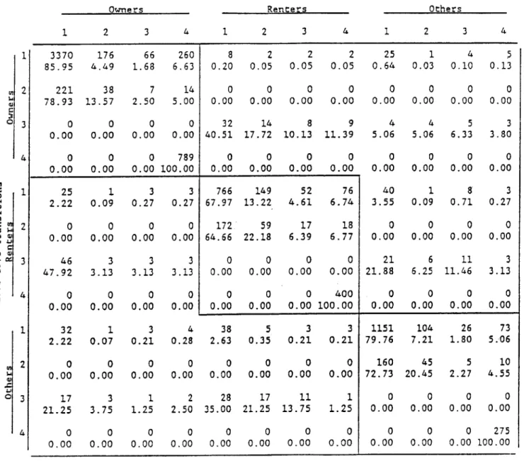
To obtain a more complete description of the transition probabilities, and to control somewhat for the heterogeneity in the data, the definition of the possible states may be expanded to add the three different tenure types for each state (i.e. there are now 12 states). The resulting matrices are found in Tables 2-5. The blocks on the main diagonals in Tables 2-5 cor-respond to the same tenure type (i.e. the upper left hand block corcor-responds to those who were owners at the beginning of both of the periods in the table during which a housing decision was made). For example, the (2,1) element of the matrix in Table 3 contains those households who owned their residence in 1971, moved to owning another residence between 1971 and 1973, and then did not move between 1973 and 1975. _{As was the case with the single period}

transition probabilities given earlier, these tables show that there is a sig-nificant amount of variation in the transition probabilities for the different

tenure types. _{Given the large number of owners relative to the other tenure} types, the aggregate statistics listed in Table 1 are heavily weighted to coincide with the transition probabilities of the owners. This can be seen clearly in one of the aforementioned results, namely the difference in mortality between those who recently moved to a different tenure type and those who were in one of the two other reoccurring states. Looking at Table 3 for example, this inequality in the probability of dying holds only for the owners and not for the renters or the others. Tables 2-5 also show a large difference between owners and renters in how mobility changes over time.

TABLE 2. TRANSITION PROBABILITIES BY TENURE STATUS 1971-1973 1971-1973 Transitions Renters 1 2 3 4 1 2 3 4 1 2 3 4 4176 291 85.84 5.98 190 74.22 0 0.00 0 0.00 33 2.29 0 0.00 82 41.84 0 0.00 54 3.03 0 0.00 18 20.93 0 0.00 40 15.63 0 0.00 0 0.00 4 0.28 0 0.00 20 10.20 0 0.00 90 238 1.85 4.89 10 3.91 0 0.00 16 6.25 0 0.00 0 246 0.00 100.00 3 0.21 0 0.00 3 1.53 0 0.00 2 0.14 0 0.00 7 3.57 0 0.00 + 2 3 3 0.11 0.17 0.17 0 0.00 0 0.00 1 4 1.16 4.65 0 0.00 0 0.00 0 0.00 2 2.33 0 0.00 22 0.45 0 0.00 45 34.09 0 0.00 1 0.02 0 0.00 1 0 0.02 0.00 33 3 0.68 0.06 0 0 0 0 0.00 0.00 0.00 0.00 31 23 23.48 17.42 0 0.00 0 0.00 955 195 110 66.41 13.56 7.65 217 104 55.36 26.53 0 0.00 0 0.00 49 2.75 0 0.00 28 32.56 0 0.00 0 0.00 0 0.00 5 0.28 0 0.00 19 22.09 0 0.00 41 10.46 0 0.00 6 4.55 0 0.00 88 6.12 30 7.65 0 0.00 0 147 0.00 100.00 7 0.39 0 0.00 11 12.79 0 0.00 3 0.17 0 0.00 3 3.49 0 0.00 13 9.85 0 0.00 39 2.71 0 0.00 41 20.92 2 1.52 0 0.00 2 0.14 0 0.00 4 0.08 0 0.00 .6 0.12 0 0.00 11 1 8.33 0.76 0 0.00 0 0.00 5 2 0.35 0.14 0 0.00 14 22 7.14 11.22 0 0 0.00 0.00 1416 150 79.55 8.43 78 57.35 0 0.00 0 0.00 44 32.35 0 0.00 0 0.00 0 0.00 7 3.57 0 0.00 21 67 1.18 3.76 6 4.41 0 0.00 8 5.88 0 0.00 0 0 79 0.00 0.00 100.00 1 - Stay

2 - Move to the same tenure

3 - Move to a different tenure 4 - Die Owners Others 01 1-~ 0 '.. 0% 1

-4

TABLE 3. TRANSITION PROBABILITIES BY TENURE STATUS 1973-1975

1973-1975 Transitions Renters 2 3 4 1 2 3 4 1 2 3 4 3707 222 64 244 86.07 5.15 1.49 5.67 46 13.53 0 0.00 0 0.00 6 1.76 0 0.00 18 5.29 0 0.00 0 514 0.00 100.00 4 3 0.32 0.24 0 0.00 10 5.46 0 0.00 5 0.31 0 0.00 0 0.00 6 3.28 0 0.00 2 0.16 0 0.00 5 2.73 0 0.00 18 0.42 0 0.00 42 39.25 0 0.00 4 0.09 0 0.00 12 11.21 0 0.00 2 0.05 0 0.00 -13 12.15 0 0.00 875 148 55 70.74 11.96 4.45 194 57.57 0 0.00 0 0.00 101 29.97 0 0.00 18 5.34 0 0.00 1 34 0.02 0.79 0 0.00 0 0.00 9 13 8.41 12.15 0 0.00 82 6.63 24 7.12 0 0.00 0 0 279 0.00 0.00 100.00 ______________________________________________________ + 4 4 48 0.25 0.25 2.96 0 0.00 4 2 6.06 3.03 0 0.00 0 0.00 0 0.00 0 0.00 1 25 1.52 37.88 0 0.00 0 0.00 8 0.49 0 0.00 7 0.43 0 0.00 6 9 9..09 13.64 0 0.00 0 0.00 4 0.25 0 0.00 1 1.52 0 0.00 0 0.00 25 2.02 0 0.00 37 20.22 0 0.00 1 5 5 0.02 0.12 0.12 0 0.00 0 0.00 5 9 4.67 8.41 0 0.00 0 0.00 0 0.00 4 3.74 0 0.00 1 3 3 0.08 0.24 0.24 0 0.00 0 0.00 0 0.00 6 15 5 3.28 8.20 2.73 0 0.00 1238 158 76.47 9.76 140 60.61 0 0.00 0 0.00 58 25.11 0 0.00 0 0.00 0 0.00 31 70 1.91 4.32 23 9.96 0 0.00 10 4.33 0 0.00 0 0 176 0.00 0.00 100.00 1 - Stay

2 - Move to the same tenure

3 - Move to a different tenure 4 - Die Owners 1 U, aJ Others a, 1.. C W, 0 -. 4 -V4 r-4 '.4 a% 270 79.41 0 0.00 0 0.00 36 2.91 0 0.00 99 54.10 0 0.00 42 2.59 0 0.00 18 27.27 0 0.00

~.W

TABLE 4. TRANSITION PROBABILITIES BY TENURE STATUS 1975-1977 1975-1977 Transitions Owners Renters 1 2 3 4 1 2 3 4 1 2 3 4 3370 176 85.95 4.49 221 38 78.93 13.57 0 0.00 0 0.00 25 2.22 0 0.00 46 47.92 0 0.00 0 0.00 0 0.00 1 0.09 0 0.00 3 3.13 0 0.00 32 1 2.22 0.07 0 0.00 17 21.25 0 0.00 0 0.00 3 3.75 0 0.00 66 260 1.68 6.63 7 2.50 0 0.00 14 5.00 0 0.00 0 789 0.00 100.00 3 0.27 0 0.00 3 3.13 0 0.00 3 0.21 0 0.00 3 0.27 8 0.20 0 0.00 32 40.51 0 0.00 2 0.05 0 0.00 14 17.72 0 0.00 766 149 67.97 13.22 0| 172 0.00 I 64.66 3 3.13 0 0.00 0 0.00 0 0.00 4 38 0.28 2.63 0 0.00 1 2 1.25 2.50 0 0.00 0 0.00 0 0.00 28 35.00 0 0.00 59 22.18 0 0.00 0 0.00 5 0.35 0 0.00 2 0.05 0 0.00 8 10.13 0 0.00 52 4.61 17 6.39 0 0.00 2 0.05 0 0.00 9 11.39 0 0.00 76 6.74 18 6.77 0 0.00 0 400 0.00 100.00 3 0.21 0 0.00 17 11 21.25 13.75 0 0 0.00 0.00 25 0.64 0 0.00 4 5.06 0 0.00 40 3.55 0 0.00 1 4 0.03 0.10 0 0.00 0 0.00 4 5 5.06 6.33 0 0.00 1 0.09 0 0.00 21 6 21.88 6.25 0 0.00 3

I

2 - Move to the same tenure 3 - Move to a different tenure 4 - Die U7 In J.J r. 0 "I 41 5 0.13 0 0.00 3 3.80 0 0.00 3 0.27 0 0.00 3 3.13 0 0.00 73 5.06 10 4.55 0 0.00 Ifl 0

--...

if

TABLE 5. TRANSITION PROBABILITIES BY TENURE STATUS 1977-1979 1977-1979 Transitions Renters 1 2 3 4 1 2 3 4 1 2 3 4 3027 142 84.96 3.99 173 79.36 0 0.00 0 0.00 15 1.52 0 0.00 23 10.55 0 0.00 0 0.00 0 0.00 0 0.00 80 272 2.25 7.63 8 3.67 0 0.00 14 6.42 0 0.00 0 1085 0.00 100.00 2 0.20 0 0.00 49 1 3 54.44 1.11 3.33 0 0.00 22 1.61 0 0.00 12 22.22 0 0.00 0 0.00 1 0.07 0 0.00 2 3.70 0 0.00 0 0.00 2 0.15 0 0.00 3 5.56 0 0.00 0 0.00 0 0.00 4 4.44 0 0.00 0 0.00 0 0.00 1* 10 0.28 0 0.00 40 53.33 0 0.00 1 1 3 0.03 0.03 0.08 0 0.00 5 6.67 0 0.00 703 122 71.23 12.36 159 49 68.53 21.12 0 0.00 0 0.00 24 1.75 0 0.00 0 26 0.00 48.15 0 0 0.00 0.00 0 0.00 20 0.56 0 0.00 0 0 0 0 0.00 0.00 0.00 0.00 8 10.67 0 0.00 5 12 6.67 16.00 0 0.00 34 81 3.44 8.21 8 3.45 0 0.00 16 6.90 0 0.00 0 0 511 0.00 0.00 100.00 3 0.22 0 0.00 4 0.29 0 0.00 1 0.07 0 0.00 22 2.23 0 0.00 18 20.00 0 0.00 1105 80.77 0 116 0.00 71.17 7 1 3 12.96 1.85 5.56 0 0 0 0.00 0.00 0.00 0 0.00 0 0.00 0 0.00 0 0.00 2 0.06 0 0.00 3 4.00 0 0.00 1 4. 0.10 0.41 0 0.00 4 4.44 0 0.00 99 7.24 29 17.79 0 0.00 8 8.89 0 0.00 .5 0.14 0 0.00 2 2.67 0 0.00 3 0.30 0 0.00 3 3.33 0 0.00 21 86 1.54 6.29 6 3.68 0 0 0.00 0.00 0 0.00 12 7.36 0 0.00 0 374 0.00 100.00 1 - Stay

2 - Move to the same tenure 3 - Move to a different tenure 4 - Die Owners Others r. 0 -p-I

.

Therefore, any structural model of the elderly's housing decisions must be able to both incorporate the heterogeneity that exists among households and explain why the elderly become less mobile over time.

2. Household's Decision

When a household considers whether or not to move, the decision involves weighing the gains and the costs associated with moving. The gains may be in terms of location (e.g. weather, proximity to family), "more appropriate" housing, or monetary considerations. The costs include both the observed costs associated with physically moving a household and the unobserved psycho-logical costs associated with leaving a residence and starting anew (these psychological costs include something that has been referred to as an attach-ment effect, see Venti and Wise(1984)).

An easy way to visualize the way in which a household compares the costs and gains associated with moving is to imagine a household first forming expectations of what life would be like (i.e. what the utility streams would be) both from moving to a different housing situation and from staying at its current residence, and then comparing the differences between these two

situations. _{Whenever the utility from moving is less than it would have been} from staying, the difference is considered to be a cost because the household is worse off, and whenever the utility from moving is greater than it would have been from staying, the difference is considered to be a gain. The gains and losses associated with a move and how they change with time are

repre-A

sented by the two shaded areas in Figure 2, where U is the expected utility

A

A

expected utility level of a household if it moves, T(x) is the expected date of death, and t is date at which the household starts the moving process. Note that this graph will look different for each household

0.

Not only must the gains and the losses be weighed, but the timing of those gains and losses must also be considered. The time horizon plays an important role here, because while most of the costs are realized initially, the gains accrue over time. Thus, the amount of time until death (length of the time horizon) is very important in the move/stay decision, since the length of the time horizon will indicate how much time a household has to enjoy the gains from a move. Therefore, the decision of whether or not to move must be a comparison of the discounted costs versus the discounted gains.

3. Structural Model

When a household is making a decision as to whether the discounted gains are greater than the discounted costs, the comparison is based on what the household believes about the future. _{Since one household's expectations about}

10 _{It is not necessarily the case that}

0

0m

0s

11 _{For example, how quickly a household becomes integrated}

into their new community (a difference in psychological costs) is represented by a change in the slope of the transition line between 0 and 0 .

U

(x)

U

(x)

(x)

U (x)

S

the future may be quite different than another household's, it is very important that the model address the move/stay decision at the household level. _{Therefore, the decision that an individual household faces as to} whether or not to move is made by the household summing up its expected

discounted costs and gains from a point t. _{until the expected death date T..} 1-0

This calculation can be represented by:

A T. (1) E. (Um(t) - U (t))e-r(t-t 0)dt > 0 i (MM - s~ t. 10

where r is the discount rate, and the households are indexed by i (represent-ing the fact that it is the household's expectations about the future that are relevant in the decision process, not what anyone else believes).1 2

While the representation in (1) may be straightforward, the move/stay decision is easier to analyze if it is broken up into the gains and the losses associated with moving. It is also necessary to divide the problem into

smaller pieces for a practical reason: it would be impossible to estimate the

A A

transition line from U to the eventual level of U for all households.

s m

Therefore, a discrete approximation is made that still allows for household differences in the costs and gains of moving.

3.1 Costs

The costs associated with moving a household primarily occur immediately

12 _{tm is taken to be the level of utility that would be realized}

by the household once it began the moving process (i.e. not the level that the

household will eventually obtain, but the instantaneous level). Therefore, the costs associated with moving will be represented by the period of time during which

0

0

following a move, with the household facing basically the same moving costs regardless of how long they remain in their new location. The costs of moving at time t are thus represented by the equation:

(2) C. _it C _ot + C Rent. _{it it} + C _2t Other. _t + B _{Blt it.} + rt_it

Cit

Cot,

repre-sents a fixed cost to moving. Rentit is an indicator variable which equals 1 if the household rents their existing living quarters and equals 0 otherwise. Therefore, Clt picks up the difference in the fixed cost of moving between owners and renters. _{C2t and Othert are equivalent to Clt and Rentit, except} they apply to the "other" category. _{-yit is an unobserved, household specific} heterogeneity term, and B t is a multiplicative factor to the household

specific effect. Finally, q it is a random disturbance term representing the fact that there may be stochastic deviations from the above representation. The heterogeneity term encompasses many different things: a household's optimism or pessimism of the future; adjustments to the fixed cost of moving term for such things as (i) the difference in the physical cost of moving across town versus across the country13 or (ii) the difference between those who are "pack rats" and accumulate many things (who therefore have higher moving costs because they have to transport more things) and those who are not. _{When (2) is used, the enclosed region in Figure 3 represents the gains}

13 _{This can be seen by realizing that the household}

who would move across the country is of a different type (i.e. a different -y. ) than the household who would only move a short distance. Thus the difietrence in

physical relocation costs would be captured by the different yit's multiplying B

14

from moving, while the costs are just a point mass at t .

3.2 Gains

It is well known that households differ in what they think the future will bring. This "feeling of the future" not only makes a difference in the

costs of moving (as used in (2)), but it also affects a household's perception

A A

of the future utility levels U and U . Thus,

y

s m 'it

A A

(Um - U s). Therefore, the gains from a move are expressed as:

A A

(3) (U _m (t) - U (t)) _s - U(X _it't ;i ) + B _2t y _it + e.

it

A A

where: U(X itt ) _{represents the difference in the utility functions U and Us}

as a function of the observed household characteristics X. , B is a multi-it' 2t

15

plicative factor to the household specific effect, and e . is a random disturbance term. The exact form of U(X itt ) is discussed later.

3.3 Discounting

To determine the total gain that a household would realize from a move, it is necessary to know not only the amplitude of the new utility level, but also the duration for which the increase would be sustained (i.e. total gain

-14 The difference in the discounted amounts of costs and gains resulting from specifying that the costs to be all up front and the gains to accrue over time will be absorbed by the coefficients in equation (2).

15

The utility function can be thought of as being additively separable between a function of characteristics that are observable, and a function of attributes that are common among households yet not observed by the resear-cher. _{The heterogeneity term then can be thought of as a representation of} the mapping from the unobservables to the real numbers.

B2 represents the difference in the multiplicative constants to the

heterogeneity terms that exist in

0

0

(gain/unit of time)*(amount of time)). The length of time that is relevant to the elderly, often referred to as the time horizon, is the expected amount of time until death.

Although a household might be able to make a good prediction of its time horizon by observing those around it in similar circumstances who are (or are not) dying, there still remains a great deal of stochastic variation in the time horizon that the household cannot control. Therefore, a method that resembles an expected value calculation is used to calculate the total gain: the gain for living until time t is calculated, weighted by the probability of surviving until time t, and then all of these weighted gains are summed.1 6 Since the gains are calculated from a point t. , the probability of survival that is used must be the probability of living until t conditioned on the fact that t is greater than or equal to t. .

Incorporating the effect of mortality with the explicit representations of the costs and gains of moving, (1) can be rewritten:

-T at

(4) E it -S!(tlt io) [U(Xit'it )+B 2tlit+6ite -r(s-t io)dsdt > E it [Ct Wit+B ltrit+git

atio _atio

17

where T is a finite upper bound on lifetimes, -S'(tlt.

)

probability density function of survival (where the conditioning is upon being

16 For a discrete example, think of getting 1 util at the beginning of each period. Your gain for living m periods would be m. Now suppose that

there are n periods, with the probability of dying in each period being equally likely. Then the total expected gain is: ZkPr(k) - (n+l)/2.

17 This T, the upper bound on lifetimes, is not to be confused with T., the actual death date of the household.