Acoustic Beamforming in Reverberant Environment
by
Joyce Lee
Submitted to the Department of Electrical Engineering and Computer Science in Partial Fulfillment of the Requirements for the
Degree of Master of Engineering in Electrical Engineering and Computer Science at the
MASSACHUSETTS INSTITUTE OF. TECHNOLOGY
May 21, 1999
@ 1999 Joyce Lee. All rights reserved.
The author hereby grants to M.I.T. permission to reproduce and distribute publicly paper and electronic copies of this thesis and to grant others the right to do so.
A uthor... ...
Department of E1ectridal Engineering and Computer Science May 21, 1999 Certified by ... :... ..
. ...
.. Rodney A. Brooks Thesis Supervisor A ccepted by ... .. ... ... Arthur C. Smith Chairman, Departmental Committee on Graduate ThesesAcoustic Beamforming in Reverberant Environment
by
Joyce Lee
Submitted to the Department of Electrical Engineering and computer Science May 21, 1999
In Partial Fulfillment of the Requirements for the Degree of Master of Engineering in Electrical Engineering and Computer Science
Abstract
The conventional approach for a beamformer to counteract the undesirable effects due to reverberation is blind deconvolution, which requires no priori information about the reverberant condition of the enclosure the beamformer is in. This project proposed a methodology for a beamformer to first learn about its reverberant environment and then perform dereverberation accordingly. The methodology was implemented and its performance was evaluated.
Thesis Supervisor: Professor Rodney A. Brooks
Title: Fujitsu Professor of Computer Science and Engineering of EECS Department Director of the M.I.T. Artificial Intelligence Laboratory
Acknowledgments
As is customary, I would like take this opportunity to thank everyone who has not only helped me through this past year with my research, but made my five years at M.I.T. an incredible experience.
I would like to express my deepest gratitude to my thesis supervisor, Professor Brooks. His technical guidance, his patience, as well as his super expeditious and through reading capability made my finishing the thesis on time a reality. In addition, I would like to thank Robert Irie, the greatest mentor one can ever hope for, who guided me through this whole project and helped me out every time I got frustrated and confused. I would not have had a clue to even approach this project without him. My appreciation also extends to all the wonderful and friendly people at Al Lab, for listening to me whine and letting me vent when I had lost my way.
Most importantly, I would like to thank my parents, whose love and support for me are simply boundless. I don't think I thank them often enough for putting up with my eccentricity and stubbornness. Warmest thanks to my brother Gideon and my sister-in-law Irene. Without Irene's regular email update, I would have simply lost touch with the rest of the family long time ago.
As for my friends, I would like to express my thanks to Piyush, who has shared my tears and my laughter over the past three years. Thanks to Tameez, who took over and redid our final project when I was simply hosed. Thanks to May, whose maternal instinct kept me alive during my crunch time. Thanks to Jeremy, who's always willing to make a KFC or an IHOP run in my hours of need. Thanks to Donald, for his ducks and crabs and fish. Thanks to Charles, for his biting sarcasm and great sense of humor. And thanks to Irene, for simply being another female I know in Course Six.
Above all, I would like to thank my Lord and Father in Heaven, whose grace has helped me to survive my journey through life.
Table of Contents
1 Introduction... 7
1.1 Background... 7
1.2 The Intelligent Examination Room Project ... 8
1.3 Overview ... 8
2 Beam form ing Theory... 10
2.1 Array Pattern... 10
2.2 Spatial Filter Design and Temporal Filter Design ... 12
2.3 Spatial Aliasing... 14
2.4 Bearnwidth Variation... 16
2.5 Localization: Generalized Cross Correlation... 18
3 Adaptive Filter Algorithm s... 20
3.1 General Least M ean Square Algorithm ... 22
3.2 Norm alized Least M ean Square Algorithm ... 22
3.3 Affine Projection Algorithm ... 23
3.4 Adaptive Filtering and Beam forming ... 24
4 Beamform er Design... 26
4.1 Overall System Design ... 26
4.2 Microphone Signal Preamplification and Over Sampling ... 27
4.3 Digital Compensation Filters ... 27
4.4 Beam form er ... 28
4.4.1 M icrophone Placement ... 29
4.4.2 Localization Using Cross-Correlation... 32
4.4.3 Delay and Sum ... 33
5 A Methodology for a Beamformer to Learn about Its Environment ... 39
6 Implem entation ... 42
6.1 Preamplification and Oversampling ... 42
6.2 Digital Compensation Filters ... 44
6.3 Training the M icrophones through Adaptive Filtering ... 44
7 Experim ental Results and Analysis ... 47
8 Conclusion ... 57
Appendix A Digital Compensation Filters... 58
A.1 MATLAB Code for evaluating the frequency responses of the microphone-preamplifier pairs and determining the frequency responses of the compensation filters 58 A.2 MATLAB Code for finding the breakpoints in the frequency responses of the compensation filters and creating the filters ... 59
Appendix B Adaptive Filtering... 61
B. 1 Affine Projection Algorithm M ATLAB Code... 61
B.2 Normalized Least Mean Square Algorithm MATLAB Code... 62
List of Figures
Figure 2.1 Plane wave propagates towards microphone array ... 11
Figure 2.2a Array pattern in u-space... 13
Figure 2.2b Array pattern in 0*-space... 14
Figure 2.3 Array pattern showing spatial aliasing ... 15
Figure 2.4a B eam at 200H z ... 16
Figure 2.4b Beam at 400Hz ... 16
Figure 2.4c Beam at 1000H z ... 17
Figure 2.4d Beam at 2000Hz ... 17
Figure 3.1 Feedback loop and the detailed look inside an adaptive filter... 21
Figure 4.1 Overall information flow of the system... 26
Figure 4.2 Information flow within the beamformer ... 28
Figure 4.3 Physical placement of the eight sensors ... 30
Figure 4.4a Widest and narrowest possible beam for sub-array 1... 31
Figure 4.4b Widest and narrowest possible beam for sub-array 2... 31
Figure 4.4c Widest and narrowest possible beam for sub-array 3... 32
Figure 4.5 Geometrical construction for delay calculation... 33
Figure 4.6a Array patterns of sub-array 1... 36
Figure 4.6b Array patterns of sub-array 2... 37
Figure 4.6c Array patterns of sub-array 3... 38
Figure 5.1 Illustration of the learning process for the beamformer ... 41
Figure 6.1 Schematic of the preamplifier ... 42
Figure 6.2 Bode diagrams of the preamplifier ... 43
Figure 7.1 Lining up in time the signal, the spectrogram, and the ERLE ... 49
Figure 7.2a AP ERLE of a 400-Hz sine wave with varying a ... 50
Figure 7.2b NLMS ERLE of a 400-Hz sine wave with varying p ... 50
Figure 7.2c Comparison between AP and NLMS for a 400-Hz sine wave ... 50
Figure 7.3a AP ERLE of vowel 'a' with varying a ... 51
Figure 7.3b NLMS ERLE of vowel 'a' with varying p ... 51
Figure 7.3c Comparison between AP and NLMS for vowel 'a'... 51
Figure 7.4a AP ERLE of vowel 'e' with varying a ... 52
Figure 7.4b NLMS ERLE of vowel 'e' with varying pt ... 52
Figure 7.4c Comparison between AP and NLMS for vowel 'e'... 52
Figure 7.5a AP ERLE of vowel 'i' with varying a ... 53
Figure 7.5b NLMS ERLE of vowel 'i' with varying p ... 53
Figure 7.5c Comparison between AP and NLMS for vowel 'i' ... 53
Figure 7.6a AP ERLE of vowel 'o' with varying a... 54
Figure 7.6b NLMS ERLE of vowel 'o' with varying p... 54
Figure 7.6c Comparison between AP and NLMS for vowel 'o' ... 54
Figure 7.8a AP ERLE of word 'Hello' with varying c ... 56
Figure 7.8b NLMS ERLE of word 'Hello' with varying p ... 56
Chapter 1
Introduction
1.1
Background
Beamforming has been employed in telecommunications radar and antenna array applications for many decades. The recent technological advancements in digital signal processors have prompted beamforming to be utilized in source location, speech
enhancement, as well as many other broadband applications. While many source location and beamforming algorithms have been developed, not too many of them yield
satisfactory real-time performance. Factors that lead to the degradation of system performance are usually background noise and reverberation.
The conventional approach to minimize the detrimental effects of reverberation often involves blind deconvolution. Blindness implies having no priori information about the reverberant characteristics of the enclosure. Blindness is often assumed so that the algorithms will be suitable for a wide variety of reverberant conditions. However, there is no rule that says one cannot first access information about the reverberant
characteristics and then perform deconvolution accordingly.
The goal of this project was to outline a methodology for a beamformer to first learn about the reverberant condition of the room during the setup stage. The information will then facilitate the beamformer to re-calibrate itself and create filters accordingly for future real-time signal processing. The conventional approach dictates blind
speech signal and then recover the future speech accordingly. As chapter 7 will show, the beamformer is capable of learning about its environment under certain conditions.
1.2 The Intelligent Examination Room Project
The research conducted for this thesis was part of the effort that went into the Intelligent Examination Room project, sponsored by Kaiser Permanente. The goal of this project is to design and implement a beamformer that is capable of:
e locating the doctor in the room
" recording the doctor speech " attenuating undesirable noise
This research project has two main focuses: vision and room acoustics. The vision part investigated ways to improve beamforming using information from a video
camera. The room acoustics part developed a methodology for a beamformer to learn about its reverberant environment a during setup stage and re-calibrate itself accordingly for future real-time signal processing.
1.3 Overview
The following gives an outline of the topics covered in this thesis:
* Chapter 2 covers the theory behind beamforming, the parallel between spatial filter design and temporal filter design, and basic localization techniques. * Chapter 3 covers the basics of adaptive filtering and outlines a few common
* Chapter 4 covers the overall system design, including mircrophone
preamplication, digital compensation filters, as well as different aspects of the beamformer design.
* Chapter 5 covers a methodology for the beamformer to learn about its reverberant environment.
* Chapter 6 covers implementation and discusses some technical issues countered.
* Chapter 7 covers experimental results and analysis.
Chapter 2
Beamforming Theory
Beamforming is a terminology given to a large collection of array processing algorithms that focus the array's signal-capturing capabilities in a pre-selected direction. The main lobe of an array's directivity pattern is called a beam, analogous to the beam of a flashlight. Delay-and-sum beamforming, a classic array signal processing algorithm, "steers". the beam to the desired direction by inserting appropriate delays into sensor outputs and summing the output signals to positively reinforce the desired signal with respect to the noise and waves from another direction.[1] One way to characterize the beam is through its array pattern. A table is included at the end of this chapter for quick equation reference.
2.1
Array Pattern
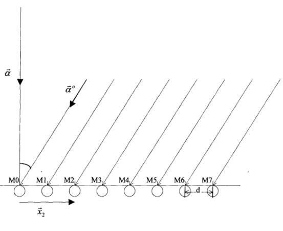
Suppose a plane wave s(t) propagates towards the beamformer with M equally-spaced (of distance d) sensors at an angle. (See Figure 2.1) The wavefield within the array's aperture can be expressed by [1]:
f(e,t)= s(t - a" - ) (2.1)
where d" is the slowness vector (with magnitude of 1/c ) that indicates propagation direction and i is the location vector.
Figure 2.1 Plane wave propagates towards microphone array
Each sensor m has an output of
y,,(t) = s(t -e - ,,,) (2.2)
The output of the delay-and-sum beamformer that assumes the propagation direction to be d (and therefore "points" towards -
a)
can be written as a weighted sum of M different sensors:M-1
z(t)= I WS(t +(a -ao) -im) (2.3)
From equation 2.3 it is easy to see that z(t) is the faithful reproduction of the original signal s(t), multiplied by a constant, when the beamformer assumes the same direction as
the propagation direction of the signal. If the original signal s(t) is further constrained to be a plane wave with only one temporal frequency co", equation 2.3 can be rewritten as
follows[1]:
z(t) = W(w'd -
E)e'"'
(2.4)where k" = cofd and W(*) represents the Fourier Transform of the sensor weights [1]: N
W(k) = Lwe k'9
m=-N
(2.5)
Equation 2.5 is also known as the array pattern. Given the signal's temporal frequency, propagation direction, and the direction the beamformer's assumed propagation direction, the array pattern can determine the output signal's amplitude and phase.
2.2
Spatial Filter Design and Temporal Filter Design
From Figure 2 and Table 1 it is can be shown that a- i = mdsinG and
C
a .. = ko = mdsino After substituting c = ' and setting u = sin0"and v = sin0 , the
array pattern W(w0d - k") becomes:
M-1 -VL!
W(co'a -
k")
= I wne ' m=0(2.6)
Lining equation 2.6 side by side with the Fourier transform X(el') of a uniformly sampled signal,
X(el'') = Ex[n]e-'" (2.7)
to I (u - v), one can get from temporal space to u-space. To get from temporal space to 9*-space, one can perform the following transformation:
04 = sin-'(' +sin9) (2.8)
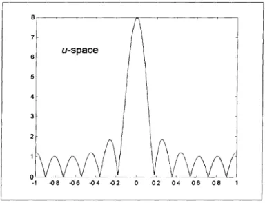
where 0" is the actual direction of propagation and 0 is the direction the beamformer assumes the wave is coming from. As a simple example, assume the following condition:
. Assumed propagation direction (not the actual one) 0 = 0 (thus v = 0)
. The number of sensors M = 8
" All weights Wm =1
. The 8 sensors are equally spaced (d = 0. 12m ) such that the set of Xm 's are:
{-3.5X, -2.5 X, -1.5 X, -0.5 X, 0.5 X , 1.5 X, 2.5 X, 3.5 x } where x is a vector whose magnitude equals to d = 0.12m .
* Frequencyf= 2000Hz, therefore 2 = c /f = 0.1 725m
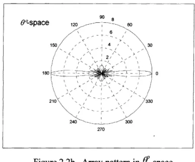
Under the above conditions, here are the plots in u-space and U-space:
90 8
Figure 2.2b Array pattern in 0 -space
2.3
Spatial Aliasing
Since the Fourier transform of the filtered signal has the periodicity of 2)r,
Vo,
I - ) must be true in order to avoid temporal aliasing. Having|0,|>-
) usually meansthe sampling frequency is not greater than the Nyquist rate and consequently temporal aliasing is introduced. Similarly, - A- ) must be true to avoid spatial aliasing in
the array pattern. Spatial aliasing usually manifests itself in the form of grating lobes in the visible region.[2] In other words, there may be extra beams pointing at directions not intended by the original design. Therefore, the inter-sensor spacing d must be chosen such that the condition I - A < r is satisfied for all combinations of u and v. After a
little mathematical manipulation, the lowest upperbound for d can be shown as (when
0o-space
0
d
-
mm (2.8)2
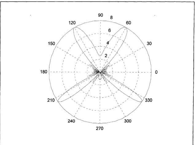
where Amin is the shortest possible wavelength (thus the highest possible frequency) for the beamformer system. Using the same example as section 2.2 where d = 0. 12m and
A = c /f = 0.1725m, one can notice that the condition in equation 2.8 has been violated.
Figure 2.3 shows the array pattern when the assumed propagation angel0 = 600.
Figure 2.3 Array pattern showing spatial aliasing 90 8
180
270
2.4 Beamwidth Variation
In the previous section, it was pointed out that the temporal frequency content (which is basically the inverse of the wavelength, multiplied by c) of the signal played an important role in determining whether there will be spatial aliasing. Upon examining equation 2.6 once more,
N _M 2,0iu_2-1v)
W(CO - k ) = we
m=-N
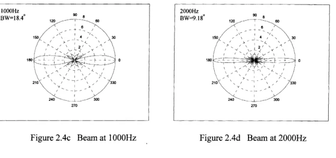
it is obvious that the array pattern is a function of the signal's wavelength (as well as temporal frequency). The beamwidth of a beamformer's main lobe is traditionally defined to be the angular difference between the two -3dB points of the main lobe and is therefore also a function of the signal's temporal frequency. Assuming all of the section 2.2 example's conditions except for the one concerning the signal's wavelength (or temporal frequency) for the example, the following figures show the array pattern and beamwidth varies with respect to the temporal frequency.
200Hz 500Hz BW=1070 " BW=37.4 8 6 6 150 / 150 50 4 30 71 / 1), I -210 3310 330 21 221 33 ~ 0 240 300 240 30 0 270 270
Figure 2.4c Beam at 1000Hz Figure 2.4d Beam at 2000Hz
There are two adverse effects due to this beamwidth variation that one should be aware of when designing a spatial filter. [2] First, the beam becomes much wider as frequency decreases and loses its resolution, as the 200Hz plot can clearly show. Second, the higher frequency content of a broadband signal is sometimes filtered due to the narrowing of the beam as frequency goes up. For instance, a signal with a frequency content between 500Hz and 1000Hz is coming in from 150. Its 1000Hz content will be significantly attenuated because the 3dB points are at -9.20 and +9.20.
It is also worth noting that one way to keep the beamwidth constant as temporal frequency changes is by changing the inter-sensor spacing d.[3] Referring back to equation 2.6 once more, one can keep the amplitude of the array pattern constant by keep
12 7du -2Adv
the argument of the exponential A - constant. Therefore, as temporal frequency decreases (and wavelength increases), inter-sensor spacing should be increased to keep the beam from widening.
1000Hz BW=18.4" 90 8 0 270 200 Hz BW--9.18' 90 180 270
2.5 Localization: Generalized Cross Correlation
As mentioned in section 2.1, the beamformer must "point" to the correct direction in order to recover the original signal z(t). After revisiting equation 2.3,
N
z(t)= LWS(t +(a -ao). ,,m)
m=-N
one can see that "pointing" at the right direction is equivalent to inserting appropriate amount of delay or advance ( T=
(a
-ao)- ,,,) for each individual sensor output. Aclassic algorithm known as the Generalized Cross-Correlation Time-Delay Estimation is based on this very idea. It can be summarized as follows [4]:
rGCC = arg(maX R (1r))
where rGCC is the optimal delay and R2 (r) is the cross-correlation between signal x, (t) and x2(t). The cross-correlation is defined as
R (t) = fx (t + )x2(r)dr
-00
Therefore, if x, (t) is a delayed version of x2(t), the cross-correlation is maximized when the optimal advance is applied to x, (t).
The Generalized Cross-Correlation Time-Delay Estimation works fairly well in an open environment with little to no echo. However, it has been shown that the
performance of this algorithm degrades drastically in reverberant enclosures. Many other variations to this classic algorithm have been proposed to minimize the adverse effect introduced by the reverberation. Most of them define a new objective function to be maximized or minimized for any given reverberant condition. [5,6]
However, once a beamformer has been constructed in a reverberant enclosure, its position is unlikely to be altered. Also, the reverberation characteristics of the enclosure are unlikely to change dramatically. Therefore, it is conceivable that a better objective function can be defined if one can first access the reverberation characteristics of the enclosure. And it was precisely this point that this project intended to prove.
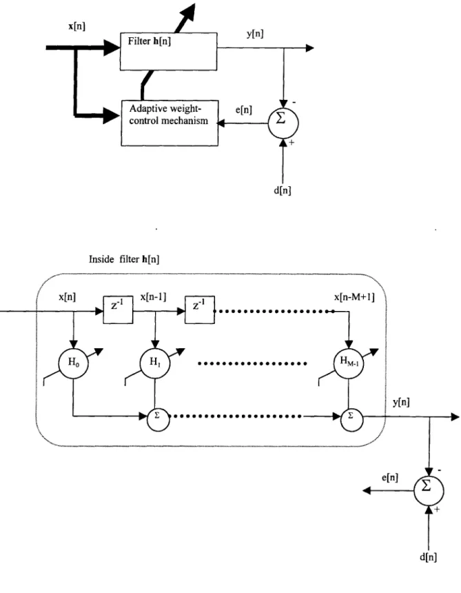
Table for Quick Equation Reference
Plane wave: s(t -
d-Slowness vector: a = k/m= 1/c
Wavenumber vector: k = ma
|k|=
2rr/AChapter 3
Adaptive Filter Algorithms
This chapter intends to give a brief synopsis of some of the more popular adaptive filter algorithms but does not go through detailed derivations of them. Most of the
outlines and conclusions about the algorithms are taken from Adaptive Filter Theory by Simon Haykin.
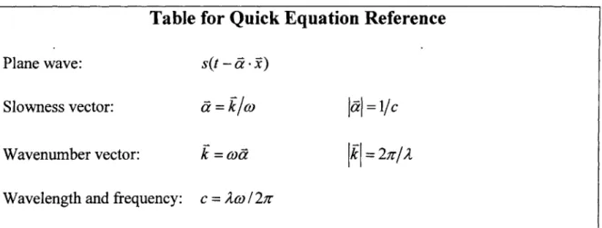
The most classic family of adaptive filter algorithms is known as the Least Mean Squares (LMS) algorithms. It is essentially a feedback control system that adjusts the coefficients of the filter until the desired response is achieved. Figure 3.1 illustrates the feedback loop as well as the detailed look inside the filter. [7]
As signal x[n] streams into the filter h[n], output y[n] is compared with the desired signal d[n] that system aims to achieve and the difference between them e[n] is fed into the adaptive weight-control mechanism, which subsequently updates the coefficients of the filter h[n]. The system usually starts off with a filter that may lead to the optimal filter. One common approach is to initialize all the filter coefficients to be zeros.
One way to visualize the convolution between input signal x[n] and the filter h[n] is matrix multiplication, as figure 3.1 has already shown. As input signal x[n] streams in, the system can take a vector of M (length of filter) most recent samples x[n] and multiply it with h[n].
x[n] y[n] + d[n] Inside filter h[n] x[n-M+I] y[n] + d[n]
3.1
General Least Mean Square Algorithm
The basic steps for a general LMS algorithm can be summarized as follows, in matrix form [7]:
1) Initialization. (n=O) Set all the filter coefficients to zero. Assume zero initial
state for input.
x[O]=h[O]=[O 0 0 ... 0]
For n>O:
2) Calculate error.
e[n]= d[n] - y[n]= d[n] h T [n]x[n]
3) Adjust filter coefficients.
h[n+l]=h[n]+2pe[n]x[n]
p is a constant that is critical in determining the convergence rate of the algorithm.
Larger p means larger incremental steps in updating the filter coefficients and can lead to faster convergence rate. However, it can also result in an increase in instantaneous error, inaccurate filter coefficients adjustment, and, potentially, divergence of the solution. As a matter of fact, the general LMS algorithm usually does not perform well in real
implementation due to the instantaneous error.
3.2 Normalized Least Mean Square Algorithm
One algorithm, known as the Normalized Least Mean Square (NLMS) algorithm, is developed to minimize the squares of the instantaneous error. The steps of NLMS can
1) Initialization. (n=O) Set all the filter coefficients to zero. Assume zero initial
state for input.
x[O]=h[O]=[O 0 0 ... 0]T
For n>0:
2) Calculate error.
e[n] = d[n] - y[n] = d[n] h T [n]x[n]
3) Adjust filter coefficients.
h[n +1] = h[n] + p e[n]x[n]
y + xT [n]X[n]
Coefficients po should be in the range between 0 and 2 for convergence rate. Coefficient
y should be a small constant and is introduced to keep the denominator from becoming
too large (and therefore keep the incremental step to a reasonable size) when input x[n] becomes too small.
3.3 Affine Projection Algorithm
One of the assumptions that both the general and Normalized LMS algorithms make is that the input x[n] and the desired signal d[n] are uncorrelated. This is hardly an assumption one can make, especially when one is dealing with reverberation. An
algorithm called the Affine Projection algorithm was developed to handle correlated d[n] and x[n]. Its strength is in its ability to uncorrelate the two signals at the cost of more computation. The Affine Projection Algorithm is summarized as follows [8]:
1) Initialization. (n=O) Set all the filter coefficients to zero. Assume zero initial
state for input.
x[O]=h[O]=[O 0 0 ... 0]T For n>O:
2) Calculate error.
e[n] = d[n] - y[n] = d[n] h T [n]x[n]
3) Uncorrelate the signal.
z[n] = x[n] - xT[n]- xI[n-]TIx[n - 1] x[n -1] x[n - 1]
4) Adjust filter coefficients.
h[n +1] = h[n] + ae[n]z[n]
y + xT [n]z[n]
3.4 Adaptive Filtering and Beamforming
Adaptive filtering is extremely popular in the mobile phone industry due to its great performance at modeling echo path. The echo, or reverberation, of a cellular phone comes mainly from the speaker (not the person, but the transmitter the person listens to). Filters are created to model echo and the modeled echo is subsequently substracted from the receiever end. This reverberation scenario is not completely dissimilar from what a beamformer has to deal with. That was why the project had chosen to implement adaptive filters as a way for the beamformer to learn about its reverberant environment. Instead of modeling the reverberation and subtracting it from the input signal x[n], this
One standard measurement of the reduction in echo, or reverberation, is called the Echo Return Loss Enhancement (ERLE) and is defined as [9]:
2
ERLE =10lo10g -d
where 0-2 and o are the variances (or powers) of the desired signal, the error,
respectively. The ERLE is analogous to the more commonly known Signal-to-Noise Ratio (SNR). The desired signal in ERLE is analogous to the signal in SNR, whereas the error is analogous to the noise.
Chapter 4
Beamformer Design
4.1
Overall System Design
0
0~aoc
0
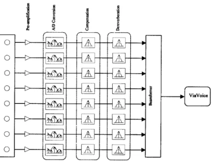
Figure 4.1 Overall information flow of the system
Figure 4.1 shows the overall information flow of the system. The eight sensors convert sound pressure into voltage and send signals to the eight pre-amplifiers, one for each sensor. The amplified signals are then converted from analog signals into digital signals and passed through another set of digital compensation filters. After that, the signals are passed through another set of filters, designed and calibrated during the setup stage to counteract the reverberation of the room. (Details of the design of these filters
summed by the beamformer, which in turn outputs the summed signal to the PC's ViaVoice speech recognition software.
4.2 Microphone Signal Preamplification and Over Sampling
Since the magnitude of the microphone output voltage is about a few millivolts, a preamplifier was built to compensate and amplify the weak signal to the line voltage level (max ±1.0 volt). The compensation stage had included a high-pass filter in order to attenuate most of the 60-Hz vibrations (i.e., air-conditioning). The high-pass filter is then cascaded with a low-pass anti-aliasing filter to keep the signals band-limited. The order of the low-pass filter was not very high because the signals, after preamplication, would be over-sampled by the A/D converter. The benefits of oversampling are twofold:1) to prevent temporal aliasing; 2) to increase the Signal-to-Noise Ratio.[10]
4.3 Digital Compensation Filters
Since no two microphones can have identical frequency responses, it is often desirable to digitally filter the sampled signal so that their frequency responses do match up to a certain reference level. A compensation filter was designed for each of the eight microphones with the reference level being the mean of the all the eight frequency responses.
4.4
Beamformer
ViaVoice
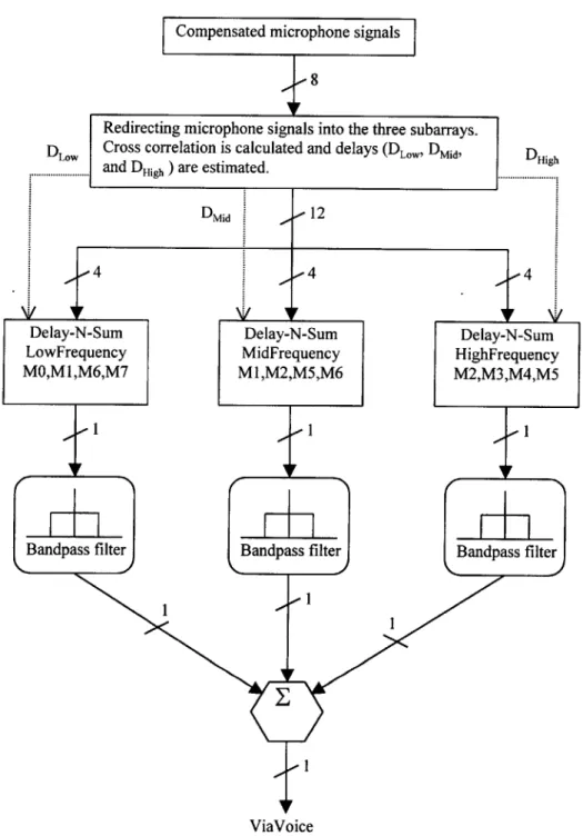
Figure 4.2 shows the overall information flow within the beamformer. In order to avoid spatial aliasing while keeping the beam to a reasonable width, the microphone sensors are grouped into three different frequency-range groups, with four sensors per group and some sensors belonging to more than one group. The details of how the sensors are grouped will be discussed in in section 4.3.1. Each group of signals is then delayed and summed accordingly. The necessary delay can be provided in one of two ways: 1) cross-correlation or 2) vision. Cross-correlation will be covered in section 4.3.3, whereas vision is the other focus of the Intelligent Examination Room and is beyond the scope of this thesis. After the delays have been inserted, the three groups of seisor signals are bandpass-filtered to the appropriate range, depending on the groups to which they belong. The three groups of signals are then recombined to form the final signal to be fed into ViaVoice.
4.4.1 Microphone Placement
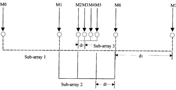
In Chapter 2, two major points regarding inter-sensor spacing were made. First, the inter-sensor spacing must be less than half of the shortest possible wavelength to avoid spatial aliasing. Second, the inter-sensor spacing should be increased in order to counteract the beamwidth widening effect. To capture signals of all frequencies without introducing spatial aliasing while still maintaining a reasonably narrow beamwidth, the eight sensors are grouped, or positioned, to form three linear equally spaced sub-arrays, each with a different distance of separation.[3] Figure 4.3 shows the physical layout of the microphone sensors where di = 9.Ocm, d2 = 4.5cm, and d3 = 1.5cm.
y
~ ~9
i
99
d3 Sub-array 31
- - 1 d
Sub-array 1 di
Sub-array 2 d2
-Figure 4.3 Physical placement of the eight sensors
The sub-arrays' highest possible frequencies can be calculated by manipulating equation
2.8:
C C
fhghest = 2)chighest A m 2*d (4.1)
and are equal to 1277Hz, 3833Hz, and 11.5kHz, respectively. Sub-array 1, which consists of sensors MO, Ml, M6, and M7, is positioned to capture the low-frequency range of 200Hz to 1200Hz. Sub-array 2, which consists of sensors Ml, M2, M5, and M6,
is responsible for the mid-frequency range of 1200Hz to 3800Hz. Sub-array 3, which consists of M2, M3, M4, and M5, takes care of high-frequency range of 3800Hz to
11000Hz. The beam patterns of the three sub-array are shown below. (BW stands for Beamwidth, in degrees) Notice that in figure 4.4a, sub-array 1 has an extremely wide beam at frequency 200 Hz. Given the number of sensors of the system, this sacrifice is hardly avoidable unless one is willing to give up the performance of the other sub-arrays.
freq = 200 BW =? 901 180! freq = 1200 BW = 30 90 1 180 | 270 270
Figure 4.4a Widest (left) and narrowest (right) possible beam for sub-array 1.
freq= 1201 BW = 94 10 3 120 60 0 6 150 30 4/ 180 - - - -- 0 210 330 240 300 270 freq = 3800 BW = 28 90 1 180 211 270
Figure 4.4b Widest (left) and narrowest (right) possible beam for sub-array 2. 0
freq= 11000 BW = 28 freq= 3801 BW = 88 90 1 1 160 08 210 0 33 - - 06 06 150 30 150 0 30 0.4 0 10 180 - - - - 0 180 -0|- -210 330 210 330 240 300 240 300 270 270
Figure 4.4c Widest (left) and narrowest (right) possible beam for sub-array 3
4.4.2 Localization Using Cross-Correlation
In chapter 2, the generalized cross-correlation algorithm used for localization was covered. To gain the highest possible resolution, the sensors farthest apart (sensor MO and M7) are chosen to perform cross-correlation. Given that the signal of sensor MO leads the signal of sensor M7 by n sample units, the incident angle 0 of the plane wave
can be computed as follows:
c *n
"= sin-'(d07 * s (4.2)
where d07 stands for the distance between sensor MO and sensor M7 and s stands for the
sampling rate. Equation 4.1 is simply a result of the mathematical manipulation and geometrical construction, as shown in Figure 4.5
Wavefront @ t= to Wavefront @ t= t-1 MO Ad = d07*sinOO
At = ti-to = Ad/c = (d07*sin40)/c
An = At*sampling rate = (d07*sinO)*sampling rate/c Ad M7 Wavefront @ t= tl
Figure 4.5 Geometrical construction for delay calculation
4.4.3 Delay and Sum
In chapter 2, it was pointed out that to steer a beamformer towards a certain direction is no more than inserting the appropriate delay or advances. (For simplicity, the rest of this section shall refer to both delay and advance as delay, for an advance is
equivalent to a negative delay.) However, since the signals are sampled at discrete-time units, inserting non-integral time-unit delay is obviously not possible. Therefore, when non-integral time-unit delay insertion is necessary, linear interpolation is employed to
beamformer is steered towards angle9 and that the delay Ano, of a particular sensor m
lands between integral time unit n and n2, the basic linear interpolation equation is as
follows:
Y(An,m)= (An,, -n,)+ y[n] (4.3)
n2 - nh
where the quantity n2 -n =1 . After setting the fraction An,,, - n to Ax,,, equation 4.3 becomes:
y(An,,,) = y[n, + 1] * Axm + y[n,] *(1 - Ax9 ,,,) (4.4)
While equation 4.4 might strike one as painfully obvious, there is some significance to it. It indicates that for every sensor m at every steering angle 9, there is an associated delay An,,, that can be represented by the sum of the integral delay n and the fractional
delay Ax,,,. Both of the integral delay and the fractional delay can be pre-computed and stored in a lookup table. Therefore, to figure out the interpolated value Y(An,,m) for sensor m at angle 9, the beamformer can simply access the pre-computed delays in the memory, as opposed to recalculating An,,, for every single sensor every time the beamformer steers towards a new angle.
To further conserve computation time and memory storage, the beampattern should once again be examined. As figures 4.4a, 4.4b, and 4.4c have shown, the smallest beam obtainable has the width of 280. What that implies is that the beamformer's
reception, when the beam is steered towards 00, remains strong (meaning within -3dB to OdB) as long as the incident angle of the plane wave stays within 0" ± 14". To cover the
figures 4.6a,b,c) Within each discrete beam, an angle that minimizes the number of interpolations is chosen as the representative angle for the beam and all the other angles will share the representative's pre-computed delays. [11] For instance, a plane wave with incident angle of 50 falls under the same beam as 0" and therefore no delays or
angle = 90 angle = 60 120 60 120 60 08 08 150 30 150 , / 30 4 / 0 2 180 T - 0 180 - - - T - - 0 AA 210 330 210 330 240 300 240 300 270 270 angle = 30 angle = 0 901 901 120 60 120 60 I 08 -1 08 06 8 06 150 30 150 30 04, 04/ 180 T I 0 160 - L - 0 210 330 210 330 240 300 240 300 270 270 angle = -30 angle = -60 9D1 901 120 60 120 60 08 I 08 06 06 150 030 150 / 30 04 0 2'0 210 330 210 330 240 300 240 300 270 270 angle = -90 901 120 60 8 150 30
Figure 4.6a Aray patters of sub-array 1
\120 2 \0
- ,
--_ / L I
angle = 84 angle = 56 1 1 120 60 120 60 08 0 6 06 150 > N 30 150 30 S04 4/N 004/ /0,2 N/ / N 0,,2 1N0 - - - -- 0 180 - -- 0 210 \ 330 210 330 240 300 240 300 270 270 angle = 28 angle = 0 9 1 90 1 120 60 120 60 08 08 150 >30 150 30 04 4 180 -- 0 180 - - - - 0 AN A 210 330 210 \ 330 240 300 240 300 270 270 angle = -28 angle - -56 9 1 90 1 120 60 120 60 08 1 08 150 30 150 3 06 ISO _L L -1- 0 180 - - 1- 0 210 330 210 330 240 300 240 300 270 270 angle = -84 16 1 120 60 |0 8
Figure 4.6b Array patters of sub-array 2
angle = 84 angle = 56 901 901 120 60 120 60 08 15 086N 06 150 30 150 K 30 04 4 180 T0 180 - 1- 0 210 \ 330 210 \ 330 240 300 240 300 270 270 angle = 28 angle = 0 120 60 120 60 08 08 06 06 150 \ 30 150 30 04/ N 04 ! 012 180 - - - 0 180 - - - - 0 210 330 21 330 240 300 240 300 270 270 angle = -28 angle = -56 91 901 120 60 120 60 08 08 06 06 150 N N 30 150 30 0 N0 N4 210 330 210 330 240 300 240 300 270 270 angle - -84 901 120 60 0 206 150 300 04/
0,2 Figure 4.6c Array patterns of sub-array 3
N180 -L- N /I L---0
,-Chapter
5
A Methodology for a Beamformer to Learn about
Its Environment
One can easily draw an analogy between a room and a filter. Imagine a small room. Person A claps. Person B hears the original clap and many echoes following after it. So the room basically takes the original clap signal and makes multiple scaled-down delayed versions of it. In signal processing terms, the room convolves the original signal with a train of impulses, or a filter.
The characteristics of the echoes are extremely location-dependent. If person A claps at a different location, what person B hears will be completely different, as is the
case if person B moves but person A stays. The room filtering function is basically a function of locations of the source and the microphone sensors.
To express how a room affects speech signal mathematically, one can set the original source speech signal to be s(t), the room filtering function to be h,,, (t, ,,)
where F, is a location vector from sensor m to the source, and the signal y, (t, F,,) at each
sensor m as:
Ym(t,,,)=
s(t)
* hroo,(t,F) (5.1)The distortion introduced by the sensors themselves are included as part of hroom (t, ,) for notation simplicity. To recover the original signal, an inverse filter function
s(t)= y,(t,F)* h (t,f) (5.2)
In Chapter 3, the basics of adaptive filtering were covered. By setting s(t) to be d[n] and y,,,(t,F)to be x[n], 8 different adaptive filters h[n] can be obtained for the 8 different sensors at each different location.
During setup stage, the beamformer would "learn" about its reverberant
environment. Or more accurately put, the beamformer would learn ways to combat the undesirable effect dues to reverberation. It would first be informed of the source's location. It would compare the original signal with the eight different sensor output signals and come up with a different filter for each sensor. And it would keep on "learning" and updating the filters, through adaptive filtering algorithm, until a desired performance is reached. And it would then associate those eight filters with the location it was told, store it for future use, and proceed to "learn" about the reverberant condition of the next location.
To obtain the original signal s(t) or the desired signal d[n], an extra microphone was used, in addition to the eight sensors of the beamformer. During the "learning" period, all nine microphones would sample simultaneously, with the sound source generating the original signal directly into the extra microphone.
Since all the "learning" occurs during the setup stage, there is no real constraint in terms of convergence rate. Therefore, the Affine Projection Algorithm was implemented for its ability to whiten the correlated speech signal. Normalized Least Mean Square Algorithm was also implemented to serve as part of the comparative analysis.
after the setup period, the beamformer would choose from its memory the set of filters for the location that is closest to the speaker's location. There is an obvious tradeoff between the beamformer's performance in dereverberation and the amount of time that is available for setup. The choice would be up to the user. Figure 5.1 summarizes the whole learning process.
Select a set of locations for beamformer to learn about.
Beamformer picks an untrained location and steers towards it.
Sensors record signals from the chosen location.
Beamformer learns to counteract the reverberation condition of the location through adaptive filtering.
Beamformer stores the the location and its associated filters in its memory
Chapter 6
Implementation
6.1
Preamplification and Oversampling
220k 220k 2.2k 5.6k 15pF 1OnF 10k
Figure 6.1 Schematic of the preamplifier
Figure 6.1 shows the schematic of the preamplifier. Each preamplifier consists of two stages and is powered by a 5 DC volt power supply. The two 220-kn resistors in series create a virtual ground of 2.5 volt to allow full (positive and negative) swing of the microphone signals. In the first stage a National Semiconductor LM6144AIN operational amplifier, which amplifies the microphone signal, is cascaded with a low-pass filter with a cutoff frequency at 20kHz to prevent time-aliasing. The low-filter filter is made up of a
potentiometer. The second stage is another LM6144AIN operational amplifier, which serves as voltage-follower, cascaded with a high-pass filter, which filters out any
frequency below 100 Hz. The high-pass filter is made up of a 10-nF capacitor and a
150-kQ resistor. Since the preamplifier's output is subsequently sampled by the Signalogic Sig32C system board's A/D converter which takes input of ± 1 volt, the high-pass filter
also helps remove the virtual ground introduced at the first stage. (The Signalogic
Sig32C system board is a board consists of a 8-channel A/D converter that converts
analog signal to digital signal and a digital signal processor which performs the beamforming.) Figure 6.2 shows the Bode diagrams of the frequency response of the preamplifier. Notice that the higher cutoff frequency end does not have as steep roll-off as the lower cutoff frequency end. The low-pass filter was mainly designed to keep the
signal band-limited. The A/D converter already has 64x oversampling that will take care of the temporal aliasing, provided that the signal is not completely band-unlimited. As a result, building a higher-order low-pass filter for the purpose of avoiding temporal aliasing would simply be redundant.
6.2
Digital Compensation Filters
As mentioned in chapter 4, no two electronic components have identical responses. To compensate for the difference in the frequency response of the eight microphone-preamplifier pairs, digital compensation filters were implemented.
To determine the frequency response of the eight pairs, one microphone at a time was placed directly in front of a speaker to record a logarithmic chirp. A logarithmic chirp is basically a signal that sweeps through the pre-designated range of frequency (in this case, from 200Hz to 10kHz) logarithmically. And the reason the chirp was
logarithmic, as opposed to linear, was to get higher resolution in the lower frequency range, where most speech occurs.
After the frequency responses of all eight microphone-preamplifiers have been determined, eight compensation filters were designed on MATLAB to get the individual microphone-preamplifier pairs to match the mean frequency response of the eight pairs. Appendix A includes all the MATLAB files used to determine the original responses as well as files used to design the compensation filters.
6.3
Training the Microphones through Adaptive Filtering
As mentioned in chapter 5, a reference signal d[n] was necessary for the eight sensor signals xm[n] to adapt to it. A headset microphone was originally employed to serve as the reference signal. The signals sampled by the eight microphones were sampled through a DOS program HSMacro whereas the signal sampled by the headset microphone was sampled through the software Goldwave. Immediately two problems
the array sensors and the headset microphone. With the foam on the headset microphone, damping was introduced and the phase of the signal was modified, in addition to its magnitude. The second problem was even more severe. Because the array sensor signals and the headset microphone signal were sampled by two different programs, the
simultaneity was lost. It was difficult to keep track of the exact delay between the
activation of Goldwave and the activation of HSMacro, since both of them were activated manually. Simultaneity is critical in determining the echo-path. Without it, the filters were simply useless.
To circumvent the simultaneity problem, the headset microphone were discarded and one of the array sensors were used to replace it. The reference sensor was placed directly in front of the sound source and the rest of the array sensors were mounted on the wall. Different kinds of signals were recorded simultaneously by the reference sensor and the array sensors. The kinds of signals include:
" Sinusoidal wave of 400Hz " Vowels: a, e, i, o, u " Single word: Hello
After the signals were recorded, adaptive filters were implemented on MATLAB following the Normalized Least Mean Square (NLMS) algorithm and Affine Projection (AP) algorithm as outlined in chapter 3. Different values for the convergence factors a and p were used to see their effects on the convergence rate as well as performance. For the detailed MATLAB code, see Appendix B.
To observe the trend of the Echo Return Loss Enhancement over time, the powers of a frame size of 500 most recent samples of desired signal d[n] and echo residual e[n]
were calculated for every step size of 250 samples. As chapter 7 will show, the ERLE did increase over time, with the ERLE of some signals more so than the others.
Chapter
7
Experimental Results and Analysis
As previously mentioned in chapter 3, one way to measure the performance of a echo-canceling adaptive filter is through the Echo Return Loss Enhancement (ERLE). This chapter shows the ERLE of the Affine Projection (AP) algorithm as well the ERLE of the Normalized Least Mean Square (NLMS) algorithm with different convergence factors (a for AP, m for NLMS) of varying values (0.01, 0.1, 0.9). The graphs of the ERLE's are attached at the end of this chapter. All 'a'-graphs show the ERLE of the AP algorithm. All 'b'-graphs show the ERLE of the NLMS algorithm. All 'c'-graphs compare the best AP's ERLE with the best NLSM's ERLE, with best meaning the best out of the three ERLE's with different values for the convergence factors.
The ERLE's with 400-Hz sinusoidal signals (Figures 7.2a, 7.2b, 7.2c) and the ERLE's of the vowels 'a' (Figures 7.3a, 7.3b. 7.3c), 'e' (Figures 7.4a, 7.4b. 7.4c), 'i' (Figures 7.5a, 7.5b. 7.5c), 'o' (Figures 7.6a, 7.6b. 7.6c), 'u' (Figures 7.7a, 7.7b. 7.7c) all increase in time as predicted.
The ERLE's of the word 'Hello' (Figures 7.8a, 7.8b. 7.8c), however, may appear disconcerting. The ERLE's start off as OdB at t = 0 second and start increasing at t = 0.35
second. The ERLE's then reach their peaks, start diving down at around t = 0.8 second
and hit bottom around t = 0.9 second. Then the ERLE's increase again, only to take a
final plunge at t = 1.4 seconds. Some values of ERLE's at t = 1.5 seconds end up being
worse job than a filter than simply zeroes out all of its input. (Recall at initialization, h[0]=[0 0 0 0 0 ... 0].)
However, if one would line up in time the desired signal d[n], the spectrogram, and the ERLE (Figure 7.1 top, middle, bottom), one would realize that t = 0.8 second
marks the end of the syllable 'Hel-' and that t = 0.9 second is the beginning of the
syllable '-lo'. From the spectrogram (dark = high amplitude, light = low amplitude), one can see that the frequency content of 'Hel-' is quite different from the frequency content of '-lo'. From t = 0 second to t = 0.35 second (before 'Hel-' begins), the desired
reference microphone signal d[n] is basically low-energy white background noise, as is the array sensor signal x[n]. Consequently, the ERLE is at OdB. From t = 0.35 second on
to t = 0.8 second, the algorithm is trying to build a filter that will capture 'Hel-'. When
'-lo' begins at t = 0.9 second, the filter is not ready to capture '-lo' and as a result, the ERLE drops down. Around t = 1.4 seconds the filter has finally adapted itself to capture the syllable '-lo', but that is when '-lo' ends and the frequency content of d[n] once again changes drastically. As a result, the ERLE once again dips down. This time the filter has already adapted to capture that frequency range of '-lo' and is therefore still capturing (meaning amplifying) the white noise in that frequency range after t = 1.4 second. As a result, some of the ERLE's (note that the worst-performing ones in this case are the ones with small convergence factor) end up diving below the OdB point.
II \
II I
I1 I I I |
0. I. 0. 1 1.2 I1.4
Tim inScns(s=200z
Figure 7.1 Lining up in time the signal (top), the spectrogram (middle), and the ERLE(bottom) 0.15 0.05 0 -0.05 -0.1 -0.15 C C-C -J It Hel- -lo -17lw ~q 0.1I
AP ERLE of sinusoidal signal
Figure 7.2a
Figure 7.2b
AP ERLE of a 400-Hz sine wave with varying a NLMS ERLE of sinusoidal signal
II V
05 1 15 2 2
Time in Seconds (Fs = 22050Hz)
NLMS ERLE of a 400-Hz sine wave with varying P 16 M w0 w 0 05 1 15 2 25 3 Time in Seconds (Fs = 22050Hz) 2*-0 25 3
16 -a =001 -4 a=01 14 a =09 12 10 8 / 6 ' 4 2 / ~/ / / AP ERLE of owel A ~\ / I / /
I
II I1 / / / ~//F ~ / / / / 1 / 0 005 01 015 02 025 03 035 04 045 05 Time in Seconds (Fs = 22050Hz)Figure 7.3a, AP ERLE of vowel 'a' with varying a
Figure 7.3b NLMS ERLE of vowel 'a' with varying P
I
AP vs. NLMS0 005 01 015 0.2 025 03 035 0.4 045 05
Time in Seconds (Fs = 22050Hz)
Figure 7.3c Comparison between AP and NLMS for vowel 'a'
M wD w 15 14 13 12 - 11 S10
AP ERLE of vowel E
Time in Seconds (Fs = 22050Hz)
Figure 7.4a AP ERLE of vowel 'e' with varying a NLMS ERLE of owel E 16 14 12 10-\6/\ / \ ... ,r 8\ / 41 2-p=0 01 0 - =01 -2 0 005 01 015 02 025 03 035 04 045 05 Time in Seconds (Fs = 22050Hz)
Figure 7.4b NLMS ERLE of vowel 'e' with varying P
AP vs. NLMS
0 005 01 0.15 02 025 03 0.35 0.4 045 05
Time in Seconds (Fs = 22050Hz)
Figure 7.4c Comparison between AP and NLMS for vowel 'e'
20 5 ui - 12 w w I
Figure 7.5a AP ERLE of vowel 'i' with varying a NLMS ERLE of wel I 25 --- = 001 --p=0 1 20C1 15 -15 051 IV 0 0 05 01 0 15 0'2 025 0'3 0 '35 0'4 0 45 0 5 Time in Seconds (Fs = 22050Hz)
Figure 7.5b NLMS ERLE of vowel ' with varying P
AP ERLE of owel 0 25 20-1 5 S10--a=001 a 09 5/ 0 0 005 01 015 02 025 03 035 04 045 05 Time in Seconds (Fs = 22050Hz)
Figure 7.6a AP ERLE of vowel 'o' with varying a NLMS ERLE of owel 0
I Time in Seconds (Fs = 22050Hz)
Figure 7.6b NLMS ERLE of vowel 'o' with varying ,
S
25 AP vs. NLMS10 1
0 005 01 015 02 025 03 035 04 045 0.5
Time
in Seconds (Fs = 22050Hz)
Figure 7.6c Comparison between AP and NLMS for vowel 'o'
in w wi 20 in w w 151
Figure 7.7a AP ERLE of vowel 'u' with varying a NLMS ERLE of owel U 16 12 10 -/ \/ 2- - A= 001 _ -- P=01 OK~ [P=09 0 005 01 015 02 025 03 035 04 045 05 Time in Seconds (Fs = 22050Hz)
Figure 7.7b NLMS ERLE of vowel 'u' with varying ,
AP %. NLMS
10
8
aW
AP ERLE of word 'Hello' with varying a
Figure 7.8b NLMS ERLE of word 'Hello' with varying P NLMS ERLE of word HELLO
w W
Time in Seconds (Fs = 22050Hz)
Chapter 8
Conclusion
As the experimental results have shown, the strength of the adaptive filtering lies in its ability to adapt to the desired signal and change in time. An optimal filter for the first quarter of a second may be less than optimal for the next quarter of a second. Therefore, adaptive filtering was not the best way to accomplish what the project originally intended: to create for each sensor a single filter whose performance is time and signal independent. However, there is still potential utilization for this design. For example, this design will be most applicable for activating the beamformer from its idle state. Suppose the filters are adapted to the word "start" or "begin" or words with one or two syllables during the setup stage. For words with two or more syllables or words with fluctuations in frequency content, two or more filters (i.e. one for "be-" and one for "-gin") will have to be stored in memory and they must be switched from one to the other after a certain time lapse. While the beamformer is idling, these filters will be employed to specifically pick up the activation word. Since the filters are designed to pick up and amplify the frequency content of the activation word, words other than the activation word (or words with other frequency content) will be attenuated. Therefore the
beamformer will only turn on when the specific activation word is spoken by the specific speaker who trained it during the setup stage.
Appendix A
Digital Compensation Filters
A.1 MATLAB Code for evaluating the frequency responses of
the microphone-preamplifier pairs and determining the
frequency responses of the compensation filters
load MFT/mft0file; load MFT/mftlfile; load MFT/mft2file; load MFT/mft3file; load MFT/mft4file; load MFT/mft5file; load MFT/mft6file; load MFT/mft7file; meanfilt = mean(abs([mftO; mftl; mft2; mft3; mft4; mft5; mft6; mft7]), 1); fq = linspace(0, 44100, 441001); fo fi f2 f3 f4 f5 f6 f7 meanfilt./abs(mft0) meanfilt./abs(mftl) meanfilt./abs(mft2) meanfilt./abs(mft3) meanfilt./abs(mft4) meanfilt./abs(mft5) meanfilt./abs(mft6) meanfilt./abs(mft7) MFT/filt0 fO MFT/filt fl MFT/filt2 f2 MFT/filt3 f3 MFT/filt4 f4 MFT/filt5 f5 MFT/filt6 f6 MFT/filt7 f7 MFT/meanfilt fq; fq; fq; fq; fq; fq; fq; fq; meanfilt fq; save save save save save save save save save
A.2 MATLAB Code for finding the breakpoints in the
frequency responses of the compensation filters and creating
the filters
clear; LoadFiltX; [fq0c, mag0c] = DwnSampMFT2(fO); F = [fq0c 9000 11025]/11025; M = [mag0c 0 0]; BO = fir2(99, F, M); BFT(1,:) =fft(BO, 400); [fqlc, maglc] = DwnSampMFT2(fl); F = [fqlc 9000 11025]/11025; M = [magic 0 0]; B1 = fir2(99, F, M); BFT(2,:) =fft(B1, 400); [fq2c, mag2c] = DwnSampMFT2(f2); F = [fq2c 9000 11025]/11025; M = [mag2c 0 0]; B2 = fir2(99, F, M); BFT(3,:) =fft(B2, 400); [fq3c, mag3c] = DwnSampMFT2(f3); F = [fq3c 9000 11025]/11025; M = [mag3c 0 0]; B3 = fir2(99, F, M); BFT(4,:) =fft(B3, 400); [fq4c, mag4c] = DwnSampMFT2(f4); F = [fq4c 9000 11025]/11025; M = [mag4c 0 0]; B4 = fir2(99, F, M); BFT(5,:) =fft(B4, 400); [fq5c, mag5c] = DwnSampMFT2(f5); F = [fq5c 9000 11025]/11025; M = [mag5c 0 0]; B5 = fir2(99, F, M); BFT(6,:) =fft(B5, 400); [fq6c, mag6c] = DwnSampMFT2(f6); F = [fq6c 9000 11025]/11025; M = [mag6c 0 0]; B6 = fir2(99, F, M); BFT(7,:) =fft(B6, 400); [fq7c, mag7c] = DwnSampMFT2(f7); F = [fq7c 9000 11025]/11025; M = [mag7c 0 0]; B7 = fir2(99, F, M); BFT(8,:) =fft(B7, 400); Bfir = [B0; B1; B2; B3; B4; B5; B6; B7];# LoadFiltX.m load MFT/filt0; load MFT/filtl; load MFT/filt2; load MFT/filt3; load MFT/filt4; load MFT/filt5; load MFT/filt6; load MFT/filt7; ####################### # DwnSampMFT2 #
function [freq, Mag] = DwnSampMFT2(mfilter);
freq(1:2) = [0 100]; Mag(1:2) = [0 0]; count=2; while freq(count)<2200, count=count+1; freq(count)= freq(count-1)+100; sampindex = freq(count)*10; Mag(count) = mean(mfilter(sampindex:samp_index+999),2); end while freq(count)<5200, count=count+1; freq(count)= freq(count-1)+500; sampindex = freq(count)*10;
Mag(count) = mean(mfilter(samp_index:samp index+4999),2); end
while freq(count)<8200, count=count+1;
freq(count)=freq(count-1)+1000; sampindex = freq(count)*10;
Mag(count) = mean(mfilter(samp_index:samp index+9999),2); end
Appendix B
Adaptive Filtering
B.1 Affine Projection Algorithm MATLAB Code
rawd = wavread('../Ada3Wave/b37.wav', [1 22050*1.5]); rawx = wavread('../Ada3Wave/b33.wav', [1 22050*1.5]); maxx = max(abs(rawx)); maxd = max(abs(rawd)); d = rawd*maxx/maxd; filtlength = 500; alpha = 0.9; gamma = 1; NumIteration = length(rawd);padded x = [zeros(filtlength-1, 1); rawx]; % n=0, initialization x = zeros(filt length, 1); h = zeros(filtlength, 1); % n=l, prevx = x; x = padded x(1:filtlength); e(1) = d(1)-h'*x; z =x; h = h +(alpha*e(1)*z)/(l+x'*z); % n=2 and so on for n=2:NumIteration if mod(n, 1000)==0, n count = round(n/1000); hh500(:,count)=h; end prevx = x; x = paddedx(n:n+filtlength-1); e(n) = d(n)-h'*x; z = x - ((x'*prevx)/(prevx'*prevx))*prevx; h = h + (alpha*e(n)*z)/(gamma+x'*z); end hh500(:,count+1) = h; eh500 = e; dhello =d;
save Mh500 hh500 eh500 dhello;