Environmental Satisfaction in Open-Plan Environments: 5. Workstation and Physical Condition Effects

(1)

Publisher’s version / Version de l'éditeur:

Vous avez des questions? Nous pouvons vous aider. Pour communiquer directement avec un auteur, consultez la

première page de la revue dans laquelle son article a été publié afin de trouver ses coordonnées. Si vous n’arrivez pas à les repérer, communiquez avec nous à PublicationsArchive-ArchivesPublications@nrc-cnrc.gc.ca.

Questions? Contact the NRC Publications Archive team at

PublicationsArchive-ArchivesPublications@nrc-cnrc.gc.ca. If you wish to email the authors directly, please see the first page of the publication for their contact information.

https://publications-cnrc.canada.ca/fra/droits

L’accès à ce site Web et l’utilisation de son contenu sont assujettis aux conditions présentées dans le site LISEZ CES CONDITIONS ATTENTIVEMENT AVANT D’UTILISER CE SITE WEB.

Research Report (National Research Council of Canada. Institute for Research in

Construction), 2003-10-20

READ THESE TERMS AND CONDITIONS CAREFULLY BEFORE USING THIS WEBSITE. https://nrc-publications.canada.ca/eng/copyright

NRC Publications Archive Record / Notice des Archives des publications du CNRC :

https://nrc-publications.canada.ca/eng/view/object/?id=587f4d52-3996-4501-8435-a4a3b887c8b0 https://publications-cnrc.canada.ca/fra/voir/objet/?id=587f4d52-3996-4501-8435-a4a3b887c8b0

Archives des publications du CNRC

For the publisher’s version, please access the DOI link below./ Pour consulter la version de l’éditeur, utilisez le lien DOI ci-dessous.

https://doi.org/10.4224/20378817

Access and use of this website and the material on it are subject to the Terms and Conditions set forth at

Environmental Satisfaction in Open-Plan Environments: 5. Workstation

and Physical Condition Effects

(2)

Environmental Satisfaction in Open-Plan Environments: 5.

Workstation and Physical Condition Effects

Veitch, J.A.; Charles, K.E.; Newsham, G.R.;

Marquardt, C.J.G.; Geerts, J.

IRC-RR-154

October 20, 2003

(3)

Environmental Satisfaction in Open-Plan Environments:

5. Workstation and Physical Condition Effects

Jennifer A. Veitch, Kate E. Charles, Guy R. Newsham, Clinton J. G. Marquardt, and Jan Geerts

Institute for Research in Construction

National Research Council Canada, Ottawa, ONT, K1A 0R6, Canada

IRC Research Report RR-154

(4)

Environmental Satisfaction in Open-Plan Environments: 5. Workstation and Physical Condition Effects

Jennifer A. Veitch, Kate E. Charles, Guy R. Newsham, Clinton J. G. Marquardt, and Jan Geerts

Executive Summary

Open-plan offices are notorious for their unpopularity with occupants. Among the most common anecdotal complaints are problems with distraction and inadequate privacy. As part of the Cost-effective Open-Plan Environments project, a field study was conducted to examine the relationships between measured physical conditions and occupant satisfaction with those conditions.

A total of 779 workstations in nine buildings were visited. Lighting, acoustic, thermal and air movement conditions were recorded along with descriptive data about workstation size, partition height, and other characteristics. Occupants completed a 27-item questionnaire simultaneously with the

measurements in their own workstations. The questionnaire covered satisfaction with individual features of the workstation, the environment overall, and the job, the rank ordered importance of seven physical features, and basic demographic characteristics. A mail-back questionnaire was provided to allow for longer comments about likes and dislikes.

This report concerns the effects of workstation physical conditions on five aspects of satisfaction: satisfaction with privacy and acoustics; satisfaction with lighting; satisfaction with ventilation; overall environmental satisfaction, and job satisfaction. Hierarchical multiple regression analyses controlled for age, job type, and gender first; then examined the effects of workstation characteristics and additional physical variables. Separate nonparametric analyses were conducted for the rank order data, and the text comments were transcribed and characterized.

Key findings are:

• Environmental conditions in the offices generally met accepted standards. This sample of

workplaces was not random, but was not chosen to exemplify good or bad workplaces. Overall, there were relatively few instances of conditions that did not meet applicable guidelines or standards.

• Having access to a window or to daylight strongly improves satisfaction with lighting. Having a

window, or daylight within 15 ft (5 m), strongly improves satisfaction with lighting. The desire for a window was a frequently mentioned comment among “things I would change” in the open-ended remarks.

• Having a window in the workstation has a detrimental effect on satisfaction with ventilation and overall environmental satisfaction. We believe this reflects the problems of heat gain and

radiant cooling. Having a window is desirable, but poor thermal conditions are not.

• Larger workstations are more satisfactory. Increasing workstation size improves satisfaction with

privacy.

• Lower partition heights appear to improve satisfaction. This finding is paradoxical, as it is

contrary to previous research and common sense, particularly with respect to privacy. We suspect that it might reflect the desire for better daylight penetration, which lower partitions afford, and to the perception that lower partitions improve ventilation.

• Concentrations of pollutants influence satisfaction with ventilation. Even at concentrations within

accepted limits, higher concentrations of carbon dioxide and other contaminants reduce satisfaction with ventilation.

The next steps for research in this area should include a wider range of variables relating to occupants, their work, and their organizations, to enable a finer-grained analysis and prescriptions for workplace design that are tailored to individuals and their specific requirements.

(5)

1.0 Introduction

Open-plan offices have become the dominant interior design strategy for North American organizations, driven both by the opportunity for lower real-estate costs and by the appeal of the notion that reducing physical barriers between individuals might also remove social barriers (Brill, Margulis, Konar, & BOSTI, 1984; Sundstrom, 1987). However, persistent problems in open-plan offices have made them fodder for cartoonists such as Scott Adams (Dilbert™) and Francesco Marciuliano and Craig Macintosh (“Sally Forth”). Among the most common complaints are lack of privacy and distractions that prevent concentration (Brill, Weidemann, & BOSTI Associates, 2001; Brookes & Kaplan, 1972; Marans & Spreckelmeyer, 1982; Mercer, 1979; Sundstrom, 1982; Zalesny & Farace, 1987). Problems with other ambient conditions have also been reported, for instance poor indoor air quality and poor thermal comfort (Hedge, 1982; Woods, Drewry, & Morey, 1987).

Two factors have consistently emerged as important influences on environmental satisfaction: the area available to each employee and the degree of enclosure. Marans and Spreckelmeyer (1982) found that the amount of space available to the employee was the strongest predictor of satisfaction with the workstation, with larger sizes being more satisfactory. Other investigators have found that workstation size predicts assessments of privacy, with larger workstations being perceived as more private (Oldham, 1988; O'Neill & Carayon, 1993). Increasing enclosure is associated with higher ratings of privacy (Oldham, 1988; Sundstrom, Burt, & Kamp, 1980) and environmental satisfaction (e.g., Brennan, Chugh, & Kline, 2002; Brill et al., 1984; Marans & Yan, 1989; Oldham, 1988).

Anecdotal reports from interior designers and facilities managers indicate that cubicles in open-plan offices are smaller than ever, and often feature lower partitions than would have been typical in the 1980s ("Space planning", 2003). Concern that these changes would result in the creation of physical conditions that would reduce environmental satisfaction was among the reasons for the creation of the Cost-effective Open-Plan Environments project in 1999. It seemed likely that reducing cubicle size would increase noise and distraction along with occupancy, and that more cubicles might mean more barriers to light and air circulation. However, we could find few investigations that reported the physical conditions in sufficient detail to predict precisely how the physical conditions might relate to environmental

satisfaction. Most of the investigations compared open-plan versus enclosed offices (e.g., Brennan et al., 2002; Mercer, 1979; Oldham & Brass, 1979; Spreckelmeyer, 1993) and in general lacked detailed measurements of physical conditions, or reported them in a manner that did not lend itself to open-plan design recommendations (e.g., Brennan et al., 2002; Marans & Spreckelmeyer, 1982; Oldham, Kulik, & Stepina, 1991; Oldham & Rotchford, 1983; Oldham & Fried, 1987; Sutton & Rafaeli, 1987). The few studies that did measure a wide range of physical conditions did not measure at individual workstations, but took averages across wide areas over periods of time (e.g., Hedge, Erickson, & Rubin, 1992).

Moreover, relatively few investigations appear to have taken place since the late 1980s, which means that most predate the change to ubiquitous personal computing.

This field investigation was designed to fill a gap in the literature, by taking detailed

measurements of both the physical conditions and the opinions of the occupants. Although a truly random sample of North American offices was not possible, the participants were from a variety of organizations, both public and private-sector, in several cities. Basic demographic variables were controlled, with the aim of providing information that could guide designers to providing open-plan office designs that will be satisfactory to the wide range of potential occupants. In addition to enlarging our understanding of how physical conditions influence environmental satisfaction, this cross-sectional field investigation is (to our knowledge) the only source of descriptive statistics on the physical conditions experienced in North American open-plan offices in the early 21st century.

(8)

2.0 Method

Detailed presentations of the method and participants in this cross-sectional field study have been presented elsewhere (Charles, Veitch, Farley, & Newsham, 2003; Veitch, Farley, & Newsham, 2002). A brief outline is provided here.

2.1 Participants

Data were collected in nine buildings between spring 2000 and spring 2002. Five of the buildings were occupied by public sector Canadian organizations. Four were occupied by private sector organizations in either Canada or the United States. The buildings were located in Ottawa and Toronto (Ontario), Montreal and Quebec City (Quebec), and in the San Francisco Bay area (California). All buildings, and the specific locations within them, were selected because they contained open-plan offices occupied by white-collar workers, and because their

management was willing to host the visit. A summary of the building characteristics at each site is shown in Table 1.

2.1.1 Buildings.

A total of 779 occupants of the nine buildings participated in the

investigation. They responded to a questionnaire about their satisfaction with the physical environment while the NRC team collected physical data pertaining to their workstations (see below). Demographic characteristics of these participants are shown in Table 2.

2.1.2 Occupants.

As may be seen in Table 2, several characteristics varied between buildings. One of the most striking differences occurred in the frequency with which respondents chose to respond to the questionnaire in English or French. We merged all the data, regardless of the language in which the questionnaire had been completed. The study had not been designed to provide data for a comparison between the two translations; moreover we were fairly confident that our translation and back-translation procedure had provided equivalent forms, given that the responses did not in general involve subtle emotional concepts that might differ from one language to another.

(9)

Table 1. Summary of site characteristics.

Building Year

Built

City Sector Visited # Floors Floor plate

(sf)

Lighting HVAC Windows Sound

1 1977 Ottawa public spring 2000 11 (4 visited) 39,000 (x 2 towers) 4' coffered prismatic fluorescent

ducted air VAV cooling / perimeter hot-water heating

non-operable no sound masking 2 1975 Toronto public summer

2000

12 (3 visited)

40,000 4' recessed parabolic cube

ducted air VAV cooling / perimeter convention heating

non-operable no sound masking 3 1975 Ottawa public spring

2000 & winter 2000 22 (4 visited) 18,000 4' recessed prismatic (some parabolic)

ducted air VAV cooling / perimeter hot and chilled water heating & cooling

non-operable sound masking in use 4 1976 Ottawa private winter

2002

15 (1 visited)

16,000 2’ x 4’ prismatic ducted air VAV cooling / perimeter hot-water heating

non-operable no sound masking 5 1994 San Rafael private spring

2002 3 (3 visited)

40,000 2’ x 4’ recessed parabolic

ducted air VAV cooling / hot-water reheat

non-operable sound masking in use 6 1984 San Rafael private spring

2002 5 (1 visited)

35,000 2’ x 4’ recessed parabolic

ducted air VAV cooling perimeter hot-water heating non-operable no sound masking 7 1916 (renovated 2000) San Francisco private spring 2002 8 (1 visited)

41,000 8’ direct/ indirect ducted air VAV operable windows

sound masking in specific locations 8 1954 Montreal public spring

2002 4 (2 visited) 6,700 50% indirect / 50% 2’x 4’ parabolic

ducted air VAV / perimeter heating non-operable no sound masking 9 1989/90 Quebec City public spring 2002 3 (3 visited)

15,300 1’ x 4’ parabolic Fan-coil with occupant-controlled ceiling vents, perimeter electric heating

non-operable no sound masking

(10)

(11)

Table 2. Demographic characteristics of participating occupants.

Site N % English % female /% male Mean age (SD)

Full sample 779 79.5 47.6 / 51.5 36.2 (10.6) Building 1 132 85.6 47.7 / 51.5 38.2 (12.7) Building 2 160 98.8 48.8 / 50.6 37.8 (9.4) Building 3 127 75.6 49.6 / 48.8 39.5 (10.1) Building 4 52 94.2 23.1 / 75.0 32.1 (8.0) Building 5 85 97.6 67.1 / 31.8 33.1 (9.6) Building 6 48 100.0 62.5 / 37.5 29.8 (9.4) Building 7 72 100.0 31.9 / 68.1 30.7 (7.3) Building 8 47 0.0 53.2 / 44.7 38.8 (9.9) Building 9 56 0.0 35.7 / 64.3 37.3 (10.1) Job Category (%)

Administration Technical Professional Management

Full sample 27.1 24.9 38.4 8.6 Building 1 18.9 11.4 68.2 0.0 Building 2 47.5 11.3 32.5 8.1 Building 3 39.4 22.8 24.4 11.8 Building 4 1.9 57.7 30.8 7.7 Building 5 20.0 20.0 41.2 17.6 Building 6 33.3 14.6 35.4 16.7 Building 7 6.9 52.8 25.0 15.3 Building 8 31.9 34.0 29.8 2.1 Building 9 10.7 42.9 46.4 0.0 Education (%)

High School Community College University courses Undergraduate Degree Graduate Degree Full sample 11.6 15.1 14.6 34.0 22.7 Building 1 9.1 8.3 13.6 30.3 37.1 Building 2 13.1 21.3 16.9 26.3 20.0 Building 3 26.8 22.8 12.6 21.3 12.6 Building 4 0.0 5.8 13.5 36.5 42.3 Building 5 4.7 3.5 12.9 58.8 17.6 Building 6 6.3 8.3 18.8 41.7 25.0 Building 7 2.8 5.6 19.4 48.6 23.6 Building 8 12.8 27.7 14.9 25.5 17.0 Building 9 14.3 30.4 8.9 35.7 10.7

Note. Percentages that do not sum to 100 are the result of rounding error and missing data.

2.2 Independent Variables

During the data collection visit, the NRC team used a specially designed and constructed cart attached to a modified office chair to take measurements of the physical conditions at the workstation. These measurements included illuminance at various points on the work surface, sound level at the approximate location of a seated occupant’s ear, temperature and air movement at head, knee, and ankle height of a seated occupant, relative humidity at torso height, and concentrations of carbon monoxide, carbon dioxide, total hydrocarbons and methane, as well as the size of the workstation, height of partitions surrounding the workstation, and number of enclosed sides of the workstation. Additional

(12)

acoustic and illuminance measurements were taken at night, with no occupants and no daylight. This equipment was described in detail by Veitch et al. (2002).

2.3 Dependent Variables

Participating occupants completed a 27-item questionnaire. It consisted of 18 individual ratings of their satisfaction with specific environmental conditions, two overall ratings of environmental

satisfaction, two items assessing job satisfaction, one set of rankings of the relative importance to that individual of 7 environmental features, and four demographic characteristics: age, sex, job type, and education level (Veitch et al., 2002).

Exploratory and confirmatory factor analyses were used to create three subscales of satisfaction from the 18 individual items (Charles et al., 2003; Veitch et al., 2002). Thus, the final set of dependent variables for this field study comprised Satisfaction with Privacy (Sat_Priv), Satisfaction with Lighting (Sat_Light), Satisfaction with Ventilation (Sat_Vent), Overall Environmental Satisfaction (OES), and Job Satisfaction (JobSatis). Each was calculated as the average of the contributing items, on scales from 1 to 7. The demographic characteristics were used as control variables in the regression analyses. Ranked importance was analysed separately and is reported below.

2.4 Procedure

Building occupants were contacted by memo or e-mail by their management prior to the visit by the NRC research team, to inform them about the investigation and to invite their participation. During the visit, a research team of two NRC staff visited individual workstations in the designated areas of the building. The team approached the occupants individually to invite their participation; over 95% agreed to participate. Having accepted the invitation, the participant was conducted to an adjacent workstation to complete the questionnaire on a handheld computer. At the same time, the NRC team replaced the participant’s usual chair with the instrumented chair and took the physical measurements of the workstation. Each workstation visit took approximately 13 minutes. At the end of the visit the team moved on to the next occupied workstation. Two teams returned to the building to take night-time

measurements of acoustic conditions and illuminances. Further details of the procedure are in Veitch et al. (2002).

Participants received no reward for participation, but both employees and management of the building received a report summarizing the physical conditions and aggregate satisfaction responses in that building.

3.0 Results and Discussion

3.1 Descriptive Statistics

As previously stated, the dependent variables were scale scores for five aspects of satisfaction, each measured on a scale from 1 to 7, with rising numbers reflecting greater satisfaction. The overall descriptive statistics are shown in Table 3. These statistics are for all cases with valid data (including cases excluded from regression analyses as univariate outliers). In general, among the aspects of the physical environment, Sat_Priv scores were lowest, and Sat_Light scores highest. JobSatis was very high, with a mean of 5.07 and median of 5.00. Over half of the sample were “satisfied” or “very satisfied” with their jobs.

(13)

Table 3. Full sample descriptive statistics for dependent variables.

Variable N Mean SD Median Minimum Maximum

SAT_PRIV 775 3.88 1.12 3.90 1.00 6.70 SAT_VENT 775 4.25 1.41 4.33 1.00 7.00 SAT_LIGHT 776 4.75 1.20 5.00 1.40 7.00 OES 745 4.05 1.31 4.00 1.00 7.00 JOBSATIS 767 5.07 1.08 5.00 1.00 7.00

From the many physical measurements we selected a subset for the regression analyses. These were selected because of their relevance to the project (workstation size and partition height), their theoretical relevance (degree of enclosure), or to cover the most important elements of the acoustic, ventilation/temperature, and lighting conditions, as identified in previous COPE research or in the scientific literature. The descriptive statistics for each variable and their definitions are provided in tables 4, 5, 6, and 7. Sample sizes differ slightly from one variable to another because of equipment failures and operator errors; these were random losses. Acoustic variables have the greatest losses because in two buildings some workstations were not available for the necessary night-time measurements.

3.1.2 Independent variables: Physical conditions.

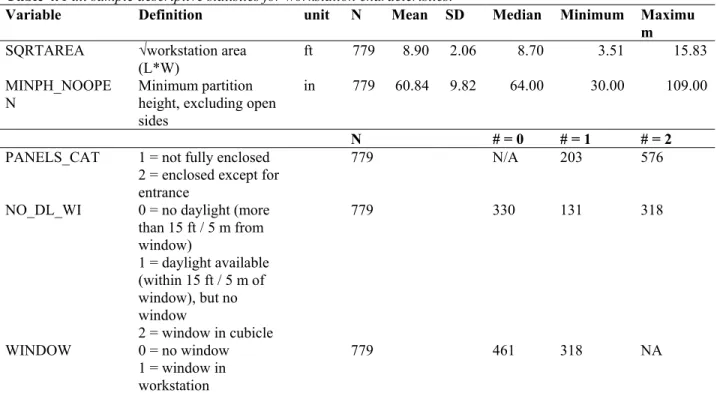
Table 4 shows the general workstation characteristics. The indicator for workstation size was the square root of the workstation area. Areas were calculated from the measured data for length and width, and corrected when the shape was known not to be square or rectangular (a few were triangular). We chose to convert to the square root for easier comparisons to other COPE project results, where square workstations were studied and results reported according to their length. For partition height, we took the height of the lowest side on which there was a partition on the basis that this was the most conservative estimate of enclosure that might affect privacy. We excluded open sides in this determination because all workstations were open on at least one side to provide an entrance, and because the degree of enclosure was separately captured. Figure 1 shows the histograms for workstation area and partition height, which were the principal variables of interest for the COPE project.

The median value of 8.70 ft for the square root of workstation area converts to approximately 76 square feet per workstation, which is within the range reported in a recent IFMA survey . In that survey, professional staff averaged 79 sf, senior clerical staff 77 sf, and general clerical staff 66 sf (our value here is across all job types).

(14)

Table 4. Full sample descriptive statistics for workstation characteristics.

Variable Definition unit N Mean SD Median Minimum Maximu

m SQRTAREA √workstation area

(L*W)

ft 779 8.90 2.06 8.70 3.51 15.83 MINPH_NOOPE

N

Minimum partition height, excluding open sides

in 779 60.84 9.82 64.00 30.00 109.00

N # = 0 # = 1 # = 2

PANELS_CAT 1 = not fully enclosed 2 = enclosed except for entrance

779 N/A 203 576

NO_DL_WI 0 = no daylight (more than 15 ft / 5 m from window) 1 = daylight available (within 15 ft / 5 m of window), but no window 2 = window in cubicle 779 330 131 318 WINDOW 0 = no window 1 = window in workstation 779 461 318 NA

Figure 1. Histograms for workstation area (SQRTAREA) and partition height (MINPH_NOOPEN).

0 1 2 3 4 5 6 7 8 9 10 11 12 13 14 15 16 17 Square Root of WS Area 0 100 200 300 C o u n t 0.0 0.1 0.2 0.3 P ro p o rti o n p e r B a r 30 38 46 54 62 70 78 86 94 102110 Minimum Partition Height 0 50 100 150 200 250 C o u n t 0.0 0.1 0.2 0.3 P ro p o rti o n p e r B a r

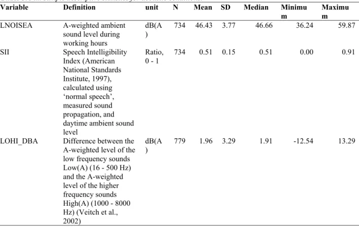
Table 5 shows the acoustic conditions. The acoustic variables used both daytime sound level measurements (excluding speech) and night-time measurements of sound propagation (cf. Veitch et al., 2002). For these analyses, we used the Speech Intelligibility Index calculation with the assumption of “normal” speech levels (American National Standards Institute, 1997). There is some evidence that actual speech in open-plan workstations is quieter than this (Warnock & Chu, 2002), in which case the true SII values would be lower. The values reported here may therefore be viewed as the worst-case scenario. The mean value for SII indicates that speech intelligibility is quite high; however, overall noise levels are in the range of desired conditions, as determined in a recent literature review (Navai & Veitch, 2003).

We also examined a new indicator of acoustic conditions, the difference between the low-frequency and high-low-frequency components of ambient noise. This characteristic was a good predictor of

(15)

acoustic satisfaction in a COPE laboratory experiment (Veitch, Bradley, Legault, Norcross, & Svec, 2002) and we wished to examine its distribution and effects in the field.

Table 5. Full sample descriptive statistics for acoustic conditions.

Variable Definition unit N Mean SD Median Minimu

m

Maximu m LNOISEA A-weighted ambient

sound level during working hours

dB(A )

734 46.43 3.77 46.66 36.24 59.87

SII Speech Intelligibility Index (American National Standards Institute, 1997), calculated using ‘normal speech’, measured sound propagation, and daytime ambient sound level

Ratio, 0 - 1

734 0.51 0.15 0.51 0.00 0.91

LOHI_DBA Difference between the A-weighted level of the low frequency sounds Low(A) (16 - 500 Hz) and the A-weighted level of the higher frequency sounds High(A) (1000 - 8000 Hz) (Veitch et al., 2002) dB(A ) 779 1.96 3.29 1.91 -12.54 13.29

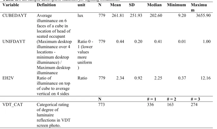
Table 6 shows the lighting conditions observed in this sample. For the lighting conditions there was one subjectively scored variable, VDT_CAT. Three independent raters viewed photos of the VDT screen in each cubicle and judged the degree to which the photo showed reflected images of luminaires. The standards for “low”, “medium”, and “high” had been produced using computer simulations of lighting installations in open-plan offices in a separate COPE task (Newsham & Sander, 2003). Interrater agreement was not as good as hoped, with 3-way agreement on only 49% of cases , an average correlation between raters of r=.72, and kappa values between any two raters in the range 0.42 - 0.50. However, Cronbach’s alpha (using each rater’s score as an item, and each workstation as a subject) was very good, being equal to 0.88. Therefore, VDT_CAT scores were created by averaging the three ratings for each workstation and binning into three categories representing the low, middle, and highest thirds.

We selected three lighting characteristics for inclusion in the regression analyses. The average illuminance reaching the eye from all directions (called CUBEDAYT here) was selected as the

illuminance value because it was the most consistent measurement, being affixed to the data-collection chair; desktop measurements proved to be less reliable because physical constraints or operator error led to variation in where the sensors were placed. There are no standards for desirable illuminance at the eye, but examination of the entire data set showed that the mean desktop illuminance was 362 lx (SD - 159) for workstations with no window, which is within recommendations for VDT offices (Illuminating Engineering Society of North America (IESNA), 1993). Depending on daylight and blind conditions, windowed workstations had desktop illuminances as high as 6700 lx. There are also no exact equivalents for our measure of desktop uniformity (UNIFDAYT) or directionality (EH2V). However, recommended practice is for fairly high desktop illuminance uniformity (Chartered Institution of Building Services Engineers (CIBSE), 1994; IESNA, 1993).

(16)

Table 6. Full sample descriptive statistics for lighting conditions.

Variable Definition unit N Mean SD Median Minimum Maximu

m CUBEDAYT Average illuminance on 6 faces of a cube in location of head of seated occupant lux 779 261.81 251.93 202.60 9.20 3655.90

UNIFDAYT (Maximum desktop illuminance over 4 locations - minimum desktop illuminance) / Maximum desktop illuminance Ratio 0 - 1 (lower values more uniform ) 779 0.44 0.20 0.41 0.01 1.00 EH2V Ratio of illuminance on top of cube to average vertical on 4 sides Ratio 779 2.34 0.92 2.25 0.37 12.16 N # = 1 # = 2 # = 3

VDT_CAT Categorical rating of degree of

luminaire

reflections in VDT screen photo.

773 336 163 274

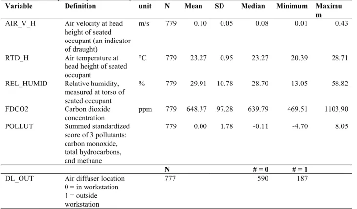
Table 7 shows the descriptive statistics for ventilation and thermal variables. Although we measured ventilation and thermal conditions at three heights, we used only the head-height measurements for further analyses. As expected, the measurements at the three heights were highly intercorrelated. It seemed likely that draught might be most problematic at the head because the majority of the offices used ceiling air diffusers, hence the choice of air velocity at that location. We chose the temperature

measurement at that location to be consistent. Relative humidity was only measured at torso height. For indoor air quality we used carbon dioxide as an indicator of ventilation system activity, and created a new variable to indicate the total concentration of other pollutants. The new variable is the sum of

standardized scores for three individual measurements; standardized scores were chosen because although each may be reported in parts per million, they differed widely in their expected distributions and in the levels at which each might be considered problematic. This new variable showed acceptable internal consistency reliability (Cronbach’s alpha = 0.64). The values of air movement, relative humidity,

temperature and carbon dioxide concentrations were all within recommended levels (American Society of Heating Refrigerating and Air Conditioning Engineers (ASHRAE), 1992; ASHRAE, 2001).

(17)

Table 7. Full sample descriptive statistics for ventilation conditions.

Variable Definition unit N Mean SD Median Minimum Maximu

m AIR_V_H Air velocity at head

height of seated occupant (an indicator of draught)

m/s 779 0.10 0.05 0.08 0.01 0.43

RTD_H Air temperature at head height of seated occupant

°C 779 23.27 0.95 23.27 20.39 28.71

REL_HUMID Relative humidity, measured at torso of seated occupant

% 779 29.91 10.78 28.70 13.05 58.82

FDCO2 Carbon dioxide concentration

ppm 779 648.37 97.28 639.79 469.51 1103.90 POLLUT Summed standardized

score of 3 pollutants: carbon monoxide, total hydrocarbons, and methane 779 0.00 1.78 -0.11 -4.70 8.05 N # = 0 # = 1

DL_OUT Air diffuser location 0 = in workstation 1 = outside workstation

777 590 187

Table 8 contains intercorrelations between all the independent

variables, using pairwise deletion of missing data. With one exception, there is no evidence of multicollinearity. The exception is the correlation of .61 between SQRTAREA and MINPH_NOOPEN, which approaches the level at which statistical problems may arise (Tabachnick & Fidell, 2001). The correlation indicates that larger workstations tend to have higher partitions. Although it might be considered an artifact of the way in which we selected buildings; we sought buildings with smaller workstations and shorter partitions to expand the original 3-building data set reported by Charles and Veitch (2002), it could also reflect a real condition in workplaces. Indeed, concerns expressed to us by design professionals about the shift to smaller workstations and lower partitions was an initial impetus behind the development of the COPE project. It seems likely that the incidence of small workstations with tall partitions is relatively rare in open-plan offices generally.

(18)

Table 8. Intercorrelations between independent variables

AGE_COMBINED GENDER ADMIN MGR PROF SQRTAREA MINPH_NOOPEN PANELS_CAT NO_DL_WI WINDOW LNOISEA SII LOHI_DBA CUBEDAYT UNIFDAYT EH2V VDT_CAT AIR_V_H RTD_H REL_HUMID FDCO2 POLLUT DL_OUT

AGE_COMBINED 1.00 GENDER 0.04 1.00 ADMIN 0.04 -0.37 1.00 MGR 0.03 0.10 -0.19 1.00 PROF 0.09 0.07 -0.49 -0.25 1.00 SQRTAREA 0.27 -0.01 0.13 -0.01 0.14 1.00 MINPH_NOOPEN 0.08 -0.01 0.06 -0.07 0.13 0.61 1.00 PANELS_CAT 0.20 -0.07 0.11 -0.04 0.13 0.49 0.36 1.00 NO_DL_WI 0.18 0.02 0.02 0.10 0.01 0.31 0.06 0.08 1.00 WINDOW 0.20 0.03 0.04 0.08 0.03 0.41 0.15 0.11 0.92 1.00 LNOISEA -0.15 0.00 0.02 0.14 -0.20 -0.36 -0.35 -0.21 0.07 0.03 1.00 SII 0.04 0.05 -0.09 -0.04 0.09 -0.06 -0.11 -0.29 0.00 0.01 -0.58 1.00 LOHI_DBA 0.06 -0.01 -0.06 -0.06 0.19 0.24 0.14 0.20 -0.11 -0.08 -0.38 0.38 1.00 CUBEDAYT 0.09 0.04 0.03 0.02 0.06 0.14 -0.06 0.03 0.37 0.37 0.01 0.06 0.01 1.00 UNIFDAYT 0.06 -0.06 0.13 -0.01 -0.06 0.02 0.02 0.06 0.08 0.11 0.05 -0.03 -0.04 0.06 1.00 EH2V -0.07 0.05 -0.03 -0.11 0.04 0.03 0.21 0.08 -0.37 -0.34 -0.12 -0.03 -0.01 -0.13 -0.28 1.00 VDT_CAT 0.02 0.01 0.00 0.00 0.00 0.09 0.06 0.04 0.00 -0.01 -0.01 -0.04 -0.08 -0.04 -0.14 0.00 1.00 AIR_V_H -0.08 0.14 0.00 0.04 -0.11 -0.16 -0.23 -0.08 -0.01 -0.03 0.17 -0.03 -0.07 0.06 0.07 -0.10 0.00 1.00 RTD_H -0.10 0.12 -0.14 -0.06 0.01 -0.33 -0.30 -0.23 -0.15 -0.18 0.12 0.13 -0.03 0.11 -0.09 0.01 -0.07 0.15 1.00 REL_HUMID 0.06 -0.01 0.15 0.01 -0.13 -0.19 -0.34 -0.03 -0.01 -0.02 0.06 0.11 -0.03 0.00 0.19 -0.13 -0.06 0.20 -0.06 1.00 FDCO2 0.04 0.06 -0.04 -0.08 0.07 -0.05 0.08 -0.01 -0.05 -0.06 -0.17 0.11 -0.13 -0.06 -0.02 0.07 0.02 -0.04 0.13 0.03 1.00 POLLUT 0.09 -0.03 0.14 -0.08 0.00 0.10 -0.01 0.11 -0.08 -0.03 -0.17 0.13 0.13 -0.01 0.13 -0.03 -0.07 0.02 -0.09 0.58 0.09 1.00 DL_OUT -0.09 -0.03 -0.07 0.11 -0.06 -0.41 -0.34 -0.18 -0.15 -0.19 0.21 0.05 -0.12 -0.05 -0.03 -0.10 -0.06 0.04 0.25 0.11 0.00 0.09 1.00

(19)

Another area of high intercorrelation is between LNOISEA and SII. This is not surprising; LNOISEA is an input to SII. Louder ambient noise can mask speech sounds.

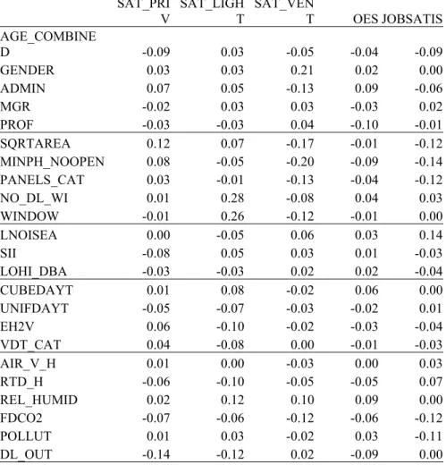
The bivariate correlations between the independent variables and the dependent variables are shown in Table 9, also using pairwise deletion of missing data. These are low, which suggests that effect sizes are likely to be small. Intercorrelations between the dependent variables are not shown, as they are reported and analyzed in more detail elsewhere (Charles et al., 2003).

Table 9. Correlations of independent variables (rows) with dependent variables (columns) SAT_PRI V SAT_LIGH T SAT_VEN T OES JOBSATIS AGE_COMBINE D -0.09 0.03 -0.05 -0.04 -0.09 GENDER 0.03 0.03 0.21 0.02 0.00 ADMIN 0.07 0.05 -0.13 0.09 -0.06 MGR -0.02 0.03 0.03 -0.03 0.02 PROF -0.03 -0.03 0.04 -0.10 -0.01 SQRTAREA 0.12 0.07 -0.17 -0.01 -0.12 MINPH_NOOPEN 0.08 -0.05 -0.20 -0.09 -0.14 PANELS_CAT 0.03 -0.01 -0.13 -0.04 -0.12 NO_DL_WI 0.01 0.28 -0.08 0.04 0.03 WINDOW -0.01 0.26 -0.12 -0.01 0.00 LNOISEA 0.00 -0.05 0.06 0.03 0.14 SII -0.08 0.05 0.03 0.01 -0.03 LOHI_DBA -0.03 -0.03 0.02 0.02 -0.04 CUBEDAYT 0.01 0.08 -0.02 0.06 0.00 UNIFDAYT -0.05 -0.07 -0.03 -0.02 0.01 EH2V 0.06 -0.10 -0.02 -0.03 -0.04 VDT_CAT 0.04 -0.08 0.00 -0.01 -0.03 AIR_V_H 0.01 0.00 -0.03 0.00 0.03 RTD_H -0.06 -0.10 -0.05 -0.05 0.07 REL_HUMID 0.02 0.12 0.10 0.09 0.00 FDCO2 -0.07 -0.06 -0.12 -0.06 -0.12 POLLUT 0.01 0.03 -0.02 0.03 -0.11 DL_OUT -0.14 -0.12 0.02 -0.09 0.00 3.2 Analytic Strategy

This investigation was a cross-sectional field survey. We sought in the analyses reported here to relate the measured physical conditions with the satisfaction of the occupants with those conditions. A separate report describes analyses involving only the physical conditions (Newsham et al., 2003a), and another reports a general model of the relationships between the questionnaire variables alone (Charles et al., 2003).

The general approach taken is hierarchical linear regression and follows generally accepted practices within the behavioural sciences, as described in standard works such as those by Kerlinger and Lee (2000), Pedhazur (1997), and Tabachnick and Fidell (2001). This section describes the criteria applied to all analyses reported here.

We examined all of the data carefully for inconsistencies and errors in data entry, and corrected these where possible, leaving data as missing if there were any question.

(20)

For the dependent variables there was very little missing data, and no evidence of any systematic missing data. We calculated scale scores as the average of available data on the contributing items, but required valid data on more than 50% of the contributing items for the scale score to be valid. Otherwise, the scale score was set to missing. This criterion resulted in four missing cases for Sat_Priv, four for Sat_Vent, three for Sat_Light, 34 for OES, and 12 for JobSatis.

We tested each dependent and independent variable for normality. Following recommendations by Kline (1997), we looked for skewness values between +3 and 3, and kurtosis values between +8 and -8. All the variables met these criteria.

We further examined the data for univariate and multivariate outliers. Univariate outliers were defined as cases on which the absolute value of the standardized score for that variable was greater than 3. These cases were omitted from analysis.

Multivariate outliers were examined for each analysis. We first ran the analysis with all cases except for the univariate outliers. We then examined the Mahalanobis distance statistic for each case. Very large values of this statistic indicate that the case is an extreme outlier and probably is having an undue effect on the outcome. Cases for which the Mahalanobis distance exceeded the critical value for that analysis were identified as multivariate outliers and excluded from analysis. (Mahalanobis distance is distributed as a chi-square and is tested against the degrees of freedom, which is the number of predictor variables in the model. We tested against a very conservative alpha of p<=.001.) For most analyses there were no multivariate outliers, and there were never more than two. We did not look for further

multivariate outliers after the first exclusion.

The results presented below are for the final sample, excluding both univariate and multivariate outliers. Because outliers were determined separately for each analysis, sample sizes vary somewhat from one analysis to another. We chose this approach to preserve as large a sample size as possible for each analysis.

The buildings were not randomly sampled; rather they were selected based on the willingness of management to provide access and on the availability of a suitable number of open-plan workstations. Later buildings were selected deliberately to ensure a broader range of workstation sizes in the overall sample. Moreover, although workstation size tends to vary within a building it is often the case that organizations use a limited range of workstation sizes and partition heights, so that the range within any one building is limited. The sample therefore has the possibility of being biased by the selection of certain organizations or certain buildings and by the confound of buildings and workstation characteristics. This means that observations from all the people in one building might be highly correlated by virtue of coming from one organization or because of commonly experienced conditions. If so, this would violate a fundamental statistical assumption, that observations are independent of one another.

3.2.2 Independence of observations..

Although the remedies for these problems are few, we did conduct a series of statistical analyses to determine the legitimacy of combing individual data from the buildings into one large sample in which we ignored the building as a variable. These tests followed the guidance of Dansereau, Alutto, and Yammarino (1984)and Yammarino and Markham (1992) regarding independence of observations. Four statistical criteria were used to examine the agreement among occupants in a building regarding the five satisfaction measurements. Traditional one-way ANOVAs were conducted in which building served as the independent variable and the five satisfaction scales served as the dependent variables. Then, using the information produced in the ANOVA (i.e., sums-of-squares and mean square), other relevant statistics were calculated (Table 10). All cases were used in these analyses, although there were 7 cases with missing data on JobSatis, 6 missing on OES, and three each on Sat_Priv, Sat-Light, and Sat_Vent.

The Intraclass Correlation Coefficient 1, or ICC(1), assesses whether occupants in the same building reliably agreed in their responses. The ICC(1) has values that range from .00 to .50, with a

(21)

median of .12 (James, 1982). An ICC(1) value of .12 or greater indicates reliable agreement. By this criterion, all of the satisfaction scales showed within-building agreement, as all had ICC(1) values >= .12.

The ICC(2) measures how reliably buildings can be differentiated based on satisfaction scores (Bartko, 1976). The closer ICC(2) is to 1.00, the better the measurement indicates whether the buildings can be reliably differentiated in terms of individual responses on the five satisfaction scales. The criterion of .85 or higher was used as an indicator of between-building differences, following Griffith (1997). Only one of the five scales passed this criterion, with Sat_Vent having ICC(2) = .861.

The E-tests (a ratio of the between-eta and within-eta) of practical significance provides an index of the magnitude of the effects (within- and between-group analysis - WABA) (Yammarino & Markham, 1992). The test of significance for the E-Test is not dependent on degrees of freedom but is geometrically based. Briefly, a 900 angle representing the relationship between two sets of scores indicates that the scores are orthogonal. The smaller the angle becomes, the stronger the observed relationship. In WABA, angles are considered for between versus within etas. The difference between the pair of angles in each case is what is tested. Thus, the larger the angular difference, the more likely that the etas are significantly different. We used the critical value for the most conservative, 300 test, E <= 0.58 (Dansereau et al., 1984). On this test all five satisfaction scales showed practical significance, meaning that the within-groups variance is greater than the between-within-groups variance. This is an indicator that observations are independent of building.

Two F tests examine the statistical significance of the between-groups versus within-groups

variance. The traditional F test compares between-group variance/within-group variance, to determine whether there are meaningful differences between buildings on the variable of interest. All five traditional

F tests are statistically significant, indicating that there are between-buildings differences in all of the

satisfaction scales. However, in cases in which the within-groups eta is the larger of the two, as in the present results (as shown by the E tests), a corrected F test is the appropriate indicator of the significance of the within-groups effect (Dansereau et al., 1984). The test is the inverse of the traditional F test. For the present results, three of the corrected F tests are statistically significant, suggesting that there are

differences between buildings in the amount of within-groups variability on these three variables (OES, Sat_Priv, and Sat_Light).

Table 10. Summary of independence analyses.

Variable ICC(1) ICC(2) etabn eta2bn etawn eta2wnE Test**

Traditional F Test Corrected F Test SAT_PRIV 0.270† 0.769 0.208 0.043 0.978 0.957 0.212 4.326* 0.231* SAT_VENT 0.408† 0.861‡ 0.264 0.070 0.964 0.930 0.274 7.195* 0.139 SAT_LIGHT 0.202† 0.695 0.182 0.033 0.983 0.967 0.185 3.280* 0.305* OES 0.240† 0.740 0.197 0.039 0.980 0.961 0.200 3.840* 0.260* JOBSATIS 0.308† 0.800 0.223 0.050 0.975 0.950 0.229 5.008* 0.200

Note. † ICC(1) >= .12. ‡ ICC(2) >= .85. ** E <= .58 indicates independence * p <= .05.

Overall, none of the five dependent variables met all four criteria for group effects. Therefore, we concluded that the assumption that observations were independent of building was met. Further analyses proceeded by combining all cases in one group, ignoring building effects.

The regression models were hierarchically structured. For all analyses, demographic control variables were entered on Step One as a block. These comprised sex (coded 0 or 1 for male or female), age (five categories entered as a continuous variable), and job type. Job type had four categories entered as three dummy codes: Admin where 1 = administrative, 0 = other; Prof where 1 = professional, 0 = other; and, Mgr, where 1 = managerial and 0 = other. The fourth category was technical.

3.2.3 Hierarchical regression models.

The order of entry of the other variables in each analysis was determined based on theoretical considerations and on guidance from the literature. Our first interest was in gross descriptors of the

(22)

workstation: workstation area, partition height, enclosure, and presence of a window. These are likely to be the most salient characteristics for occupants. Therefore, we examined the effects of workstation characteristics on all dependent variables.

The workstation characteristics were correlated with physical conditions. These relationships were examined separately and reported by Newsham et al. (2003a). For the regressions on satisfaction outcomes, we decided to control first for these workstation characteristics before adding measured physical conditions to the models. Thus, we controlled for the most salient workstation characteristics before looking to see whether the physical conditions themselves predicted additional variance. The models differed for each subset of environmental satisfaction. Thus, for Sat_Priv we looked for additional variance explained by acoustic conditions. For Sat_Light we looked at lighting conditions. For Sat_Vent we looked at ventilation and IAQ conditions. We looked at all of the physical condition models as predictors of OES and JobSatis.

3.3 Predicting Satisfaction with Privacy

Satisfaction with privacy was first regressed on workstation characteristics. For this analysis the sample size was 757 after removing cases with missing data and univariate outliers. After the control variables, workstation area (SQRTAREA) was entered as the next step, followed by enclosure (MONPH_NOOPEN and PANELS_CAT). WINDOW was the final step. Table 11 summarizes the result of this hierarchical regression.

3.3.1 Workstation characteristics.

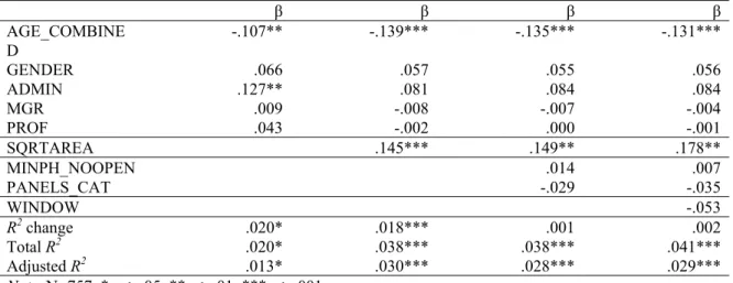
Table 11. Summary table for Sat_Priv regressed on workstation characteristics.

β β β β AGE_COMBINE D -.107** -.139*** -.135*** -.131*** GENDER .066 .057 .055 .056 ADMIN .127** .081 .084 .084 MGR .009 -.008 -.007 -.004 PROF .043 -.002 .000 -.001 SQRTAREA .145*** .149** .178** MINPH_NOOPEN .014 .007 PANELS_CAT -.029 -.035 WINDOW -.053 R2 change .020* .018*** .001 .002 Total R2 .020* .038*** .038*** .041*** Adjusted R2 .013* .030*** .028*** .029*** Note. N=757. * p<=.05. **p<=.01. ***p<=.001.

The overall model was statistically significant at all steps. Of the control variables, age persisted as a significant predictor, with younger people reporting greater satisfaction with privacy. In the first step, administrators also showed greater satisfaction with privacy, but this variable dropped out when the workstation characteristics were added. Workstation area was a significant predictor in all steps and uniquely explained 1.8% of the variance. As expected, larger workstations predicted greater satisfaction with privacy. Neither of the enclosure variables predicted satisfaction with privacy, but it would be premature to conclude that enclosure is not important because of their high correlation with workstation area (Table 8). Area is a strong predictor in this equation and could be carrying the variance for both the size and degree of enclosure.

We next looked for additional predictive power from the three physical aspects of the acoustic environment: ambient noise (LNOISEA), speech intelligibility (SII), and the relative spectral properties of the ambient noise

(23)

(LOHI_DBA).

For LNOISEA and LOHI_DBA, we thought it possible that the relationships might take a quadratic rather than a linear shape, with an intermediate value being optimal (i.e., neither too loud nor too soft, neither too rumbly nor too hissy). However, individual regressions of Sat_Priv against the quadratic shape for either LNOISEA or LOHI_DBA (always controlling for the five demographic

variables first), showed no evidence of a quadratic trend. Therefore we proceeded with linear terms only. The model entered SII first, after the control variables and the workstation characteristics.

Conversations from others are among the most frequent noise-related complaints in open-plan offices (Navai & Veitch, 2003), and we expected this to be the strongest predictor. The overall level of background noise followed, and lastly the indicator of its spectral properties. The sample size was 694 after removing cases with missing data and outliers; as noted above, some of the acoustic variables had a large amount of missing data. Table 12 summarizes the result.

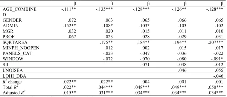
Table 12. Summary table for Sat_Priv regressed on workstation characteristics and acoustic conditions.

β β β β β AGE_COMBINE D -.111** -.135*** -.128*** -.126** -.128*** GENDER .072 .063 .065 .066 .065 ADMIN .152** .108* .103* .103 .102 MGR .032 .020 .015 .011 .010 PROF .067 .023 .028 .029 .031 SQRTAREA .175** .184** .194** .207*** MINPH_NOOPEN .012 .002 .015 .017 PANELS_CAT -.023 -.047 -.036 -.022 WINDOW -.072 -.070 -.080 -.091* SII -.071 -.038 -.012 LNOISEA .046 .055 LOHI_DBA -.046 R2 change .022** .022** .004 .001 .001 Total R2 .022** .044*** .048*** .049*** .050*** Adjusted R2 .015** .031*** .034*** .034*** .034*** Note. N=694. * p<=.05. **p<=.01. ***p<=.001.

The final model was statistically significant and explained more variance than the model with workstation characteristics only. Age and workstation area remained statistically significant predictors. In this model, with acoustic conditions controlled, presence of a window also significantly predicted

satisfaction with privacy, in an inverse direction: those with windows were less satisfied. The acoustic conditions themselves were not statistically significant predictors of satisfaction with privacy.

In our data set, satisfaction with privacy was influenced by age, workstation area, and the presence of a window. Overall, only 5% of the variance in satisfaction with privacy was explained, which is a small effect size (Cohen, 1988).

3.3.3 Discussion: Satisfaction with privacy.

Having a window reduced satisfaction with privacy to a small degree. This relationship emerged only when acoustic predictors were added to the model. It is possible that visual privacy might be compromised by a window, depending on the surroundings and the availability of blinds to control the view in. Alternatively, it is possible that a window provides a hard reflective surface that could allow more speech transmission from one workstation to another, thereby reducing speech privacy. This is consistent with the physics of sound transmission, but we know of no other satisfaction study to report such an effect.

It was not surprising to find that workstation area significantly predicted satisfaction with privacy. Larger workstations place occupants farther apart, reducing the number of people available to

(24)

overhear conversations and the number of sources of unwanted sound. The finding is consistent with other investigations, in which workplace satisfaction was greater when workstation areas were larger (Brill et al., 1984; O'Neill & Carayon, 1993; Sundstrom, Town, Brown, Forman, & McGee, 1982; Sutton & Rafaeli, 1987). Other investigations have reported separately for different job types, finding differences between them; our regression model controls for job type, yet finds the relationship nonetheless.

However, we did not find that enclosure, whether in the form of partition height or number of panels, predicted satisfaction with privacy. In this we failed to replicate previous findings that have focused on privacy as an outcome (O'Neill & Carayon, 1993; Sundstrom et al., 1980; Sundstrom et al., 1982). Two reasons might explain this. First, the high correlation between workstation area and partition height probably obscured the relationship. Second, there was little variance in the two-level categorical variable for degree of enclosure (PANELS_CAT). However, it is also possible that any partition that is not a full wall, regardless of its height, has the same effect on satisfaction with privacy (Kupritz, 2003a).

The finding that age negatively predicted satisfaction with privacy is an intriguing one with parallels in other research using qualitative methods. Kupritz (2003a) found that older workers associated having a larger office with talking privately with people, whereas younger workers did not. They also associated office location with minimizing disruptions. Privacy needs appeared to change with age, although experience rather than age per se might provide the better explanation. Given the prevalence of open-plan offices, it is possible that younger employees have had less exposure to more enclosed workplaces than older ones, and have therefore formed difference associations and expectations.

3.4 Predicting Satisfaction with Lighting

For this analysis, the sample size was 758 cases after excluding cases with missing data and outliers. Table 13 shows the result of the analysis.

3.4.1 Workstation characteristics.

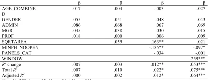
Table 13. Summary table for Sat_Light regressed on workstation characteristics.

β β β β AGE_COMBINE D .017 .004 -.003 -.027 GENDER .055 .051 .048 .043 ADMIN .086 .068 .067 .069 MGR .045 .038 .030 .015 PROF .018 .000 .006 .009 SQRTAREA .059 .163** .021 MINPH_NOOPEN -.135** -.097* PANELS_CAT -.034 -.001 WINDOW .259*** R2 change .007 .003 .012** .053*** Total R2 .007 .010 .022* .075*** Adjusted R2 .000 .002 .012* .064*** Note. N=758. * p<=.05. **p<=.01. ***p<=.001.

The final model was statistically significant and explained 7.5% of the variance, which is a small-to-medium effect size (cf. Cohen, 1988). At the final step, with WINDOW added, two predictors were statistically significant: WINDOW and MINPH_NOOPEN. Both were in the expected directions: People with a window were more satisfied with their lighting, and people with lower partitions were more satisfied. Lower partition heights allow more daylight penetration to interior workstations (Reinhart, 2002) and improve electric light distribution (Newsham & Sander, 2003), so these effects are internally consistent.

At the intermediate step, before the addition of WINDOW, both workstation area and partition height were statistically significant predictors. Workstation area dropped out at the final step, and the

(25)

regression weight for partition height also became smaller. These changes reflect the power of the WINDOW variable and the intercorrelations between the three variables. Workstation area is correlated with both partition height and presence of a window. Presence of a window has the strongest relation to satisfaction with lighting.

As for the acoustic conditions, we repeated the above analysis with additional steps for measured lighting conditions. We conducted three variations. First, we examined the result for all the workstations considered together. In this analysis we used the variable NO_DL_WI instead of the simple window/no window coding of the WINDOW variable, to account for variations in the amount of daylight that might reach a workstation adjacent to, but not having, a window.

3.4.2 Lighting conditions.

Next, we pulled out a subset consisting only of interior workstations in which no daylight could be present (those more than 15’ or 5 m from a window, NO_DL_WI = 0), and repeated the regression model (omitting, of course, NO_DL_WI as a predictor). We finally looked at the outcome for those workstations with either daylight or a window. The purpose of the regressions on the subsets was to determine whether the effects of various physical conditions model would change for occupants with no window access or daylight, relative to those with. In addition, the no-daylight model has the closest relation to physical conditions predicted by the COPE software (Newsham & Sander, 2003).

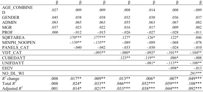
Table 14 shows the result for the overall regression, with all workstations and controlling for workstation characteristics. Although other workstation characteristics analyses had WINDOW entered with workstation size and partition height, in this case we entered it last and use the NO_DL_WI variable instead. In this analysis we first wanted to see what effect the measured lighting conditions would have, regardless of whether or not a window or daylight were present. The order of entry was determined on theoretical grounds. Each variable was a separate step. We considered that reflected images in the VDT screen might be most detrimental to satisfaction, following results obtained by Veitch and Newsham (2000). The illumination level, indexed by CUBEDAYT, entered next, as an indicator of the adequacy of the amount of light available to see. Uniformity was the third lighting variable, its importance being reflected in codes and standards (e.g., CIBSE, 1994). Directionality was the fourth variable, added because previous NRC research has suggested that it influences satisfaction with lighting (Newsham, Marchand, Svec, & Veitch, 2002). NO_DL_WI was the fifth, and last, lighting variable in this overall model. (Entering it last also facilitated comparisons with the subsample models, discussed below.)

Table 14. Summary table for Sat_Light regressed on workstation characteristics and lighting conditions.

β β β β β β β AGE_COMBINE D .027 .009 .009 .008 .014 .008 -.009 GENDER .045 .038 .038 .032 .030 .036 .037 ADMIN .083 .065 .063 .055 .063 .067 .082 MGR .037 .023 .022 .016 .017 .009 .002 PROF .000 -.012 -.015 -.026 -.027 -.028 -.011 SQRTAREA .170*** .177*** .127* .126* .122* .046 MINPH_NOOPEN -.139** -.135** -.089 -.089 -.068 -.078 PANELS_CAT -.040 -.042 -.033 -.030 -.024 -.010 VDT_CAT -.093** -.080* -.092* -.101** -.104** CUBEDAYT .123** .119** .086* -.008 UNIFDAYT -.081* -.113** -.108** EH2V -.098* -.013 NO_DL_WI .281*** R2 change .008 .017** .009** .013** .006* .007* .049*** Total R2 .008 .024* .033** .046*** .052*** .059*** .108*** Adjusted R2 .001 .014* .021** .033*** .038*** .044*** .092*** Note. N = 740. * p<=.05. **p<=.01. ***p<=.001.

(26)

The control variables alone (step one) were not significant predictors of satisfaction with lighting, but every other step achieved statistical significance. Workstation area was a significant predictor until the last step. Of the lighting variables, each added statistically significant amounts of explained variance on the step in which they entered. Each appears to have a role in explaining the variance in satisfaction with lighting. Lower levels of reflected images in computer screens, higher average global light levels, and greater desktop uniformity are all associated with higher satisfaction with lighting. Lower ratios of horizontal to vertical illuminance (EH2V) are associated with higher satisfaction (i.e., relatively more vertical than horizontal). However, at the final step with NO_DL_WI added, only VDT_CAT and uniformity remain along with NO_DL_WI as significant predictors. This final variable explains the largest amount of variance and has the largest standardized β weight. Having daylight or having a window each improve satisfaction with lighting. Relatively smaller beneficial effects are associated with lower VDT glare and greater uniformity (recall that the variable UNIFDAYT is reverse-scored, so that lower values are more uniform lighting).

Next, we separated the sample into two groups. Descriptive statistics for the three groups on the variables in this analysis are shown in Table 15. Between-group differences are apparent. Peripheral workstations are somewhat larger, have higher illuminance levels, and lower ratios of horizontal to vertical illuminance, than central workstations. The illuminance level and directionality differences are consistent with having windows providing daylight.

Table 15. Descriptive statistics for full sample and lighting subgroups.

Full Sample Central WS Peripheral WS

M SD N M SD N M SD N SAT_LIGHT 4.75 1.20 740 4.40 1.16 312 5.03 1.14 427 AGE_COMBINED 2.62 .95 740 2.50 .99 312 2.72 .91 427 GENDER 1.52 .50 740 1.52 .50 312 1.52 .50 427 ADMIN .27 .44 740 .28 .45 312 .27 .44 427 MGR .09 .28 740 .05 .21 312 .11 .32 427 PROF .39 .49 740 .39 .49 312 .38 .49 427 SQRTAREA 8.88 2.02 740 8.55 1.99 312 9.16 1.98 427 MINPH_NOOPEN 60.79 9.46 740 61.38 9.89 312 60.46 9.06 427 PANELS_CAT 1.74 .44 740 1.73 .44 312 1.75 .43 427 VDT_CAT 1.92 .88 740 1.90 .86 312 1.93 .90 427 CUBEDAYT 241.53 149.72 740 168.94 67.58 312 296.76 172.05 427 UNIFDAYT .44 .20 740 .43 .21 312 .44 .19 427 EH2V 2.32 .82 740 2.68 .79 312 2.06 .74 427 NO_DL_WI .98 .91 740 WINDOW .70 .46 427

Note. Central workstations had NO_DL_WI = 0. There were 330 of these in the full COPE sample. Peripheral

workstations had NO_DL_WI = 1 or 2. There were 449 of these in the full COPE sample.

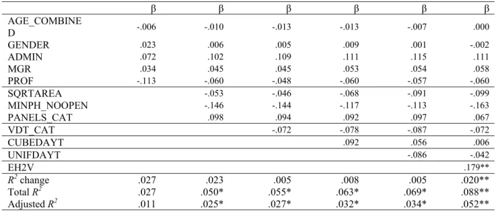
Table 16 reports the result of the regression analysis for the Central workstations. Although the model was statistically significant for steps 2-6, only one step added significantly to the explained variance, and only one variable was itself a statistically significant predictor. For those workstations without any daylight, the ratio of horizontal to vertical illuminance was a significant predictor of

satisfaction with lighting. The direction of the effect differed from the overall analysis. In this case, higher ratios were more satisfactory, indicating a preference for higher horizontal illuminance than vertical.

(27)

Table 16. Central workstations’ summary table for Sat_Light regressed on workstation characteristics and lighting conditions. β β β β β β AGE_COMBINE D -.006 -.010 -.013 -.013 -.007 GENDER .023 .006 .005 .009 -.002 ADMIN .072 .102 .109 .111 .111 MGR .034 .045 .045 .053 .058 PROF -.113 -.060 -.048 -.060 .000 .001 .115 .054 -.057 -.060 SQRTAREA -.053 -.046 -.068 -.091 -.099 MINPH_NOOPEN -.146 -.144 -.117 -.113 PANELS_CAT -.163 .098 .094 .092 .097 .067 -.072 -.087 -.072 VDT_CAT -.078 CUBEDAYT .092 .056 .006 UNIFDAYT -.086 -.042 EH2V .179** R2change .027 .023 .005 .008 .005 .020** 2 .027 .050* .055* .063* .069* .088** Adjusted R2 .011 .025* .027* .032* .034* .052** Total R Note. N = 312. * p<=.05. **p<=.01. ***p<=.001.

For the Peripheral workstations we repeated the order of entry that was used for the Central workstations, then entered WINDOW as a final step. This provided a contrast between actually having a window in the workstation (as was the case for 70% of peripheral workstations), and having daylight but no window. The results are shown in Table 17.

Table 17. Peripheral workstations’ summary table for Sat_Light regressed on workstation characteristics and

lighting conditions. β β β β β β β AGE_COMBINE D -.020 -.041 -.035 -.035 -.032 -.037 -.040 GENDER .060 .026 .027 .025 .021 .041 .041 ADMIN .097 .060 .048 .047 .057 .064 .067 MGR .049 .033 .027 .026 .022 .007 .009 PROF .087 .072 .052 .052 .049 .036 .038 SQRTAREA .196** .200** .196** .215** .209** .174* MINPH_NOOPEN -.045 -.042 -.038 -.040 -.019 -.030 PANELS_CAT -.116* -.113* -.112* -.108 -.110* -.100 VDT_CAT -.109* -.107* -.121* -.139** -.136** CUBEDAYT .012 .018 -.047 -.061 UNIFDAYT -.121* -.157** -.158** EH2V -.149** -.138* WINDOW .071 R2change .007 .023* .012* .000 .013* .015** .003 Total R2 .007 .030 .042* .042 .055* .070** .073** Adjusted R2 -.005 .012 .021* .019 .030* .043** .044** Note. N = 427. * p<=.05. **p<=.01. ***p<=.001.

For people with access to daylight or a window, although overall somewhat less variance was explained the result is more interpretable than for the Central workstations. At the end of the sixth step, without WINDOW, the model for peripheral workstations is the same as that for central workstations. Here, workstation size, the number of panels, VDT glare, uniformity and directionality were all statistically significant predictors. Satisfaction with lighting increased with larger workstations, fewer

(28)

panels, lower VDT glare, greater uniformity, and lower horizontal-to-vertical illuminance ratios. The addition of the WINDOW variable on the following step did not add significantly to the explained

variance and changed the pattern of predictor significance only for one variable: the number of panels was no longer statistically significant. This suggests that for people with some daylight, it is the physical properties of the luminous environment that principally influence satisfaction with lighting, rather than the qualities that are specific to the window, such as the view of outside that it affords.

The effect size for satisfaction with lighting falls between the ranges of small and medium-sized effects, with 10.8% of the variance explained when all workstations were considered. Slightly less variance was explained for the central (8.8%) and peripheral (7.3%) workstations considered separately.

3.4.3 Discussion: Satisfaction with lighting.

The dominant finding here is the importance of a window to satisfaction with lighting. In the workstation characteristics regression, presence of a window accounted for 5% of the variance in satisfaction with lighting, which is half of the total explained. In the form of a continuous variable that included the availability of daylight, it accounted for 5% over and above other workstation characteristics and physical measurements of lighting conditions (in the full sample regression with lighting

characteristics). Having a window, or having access to daylight, improves satisfaction with lighting. Other researchers, with other dependent measures, have also found that windows are desirable to occupants (e.g., Finnegan & Solomon, 1981; Heerwagen & Heerwagen, 1986), and that people believe that working under natural daylight is better for health and well-being than electric light (Veitch & Gifford, 1996; Veitch, Hine, & Gifford, 1993).

Satisfaction with lighting was also a function of reflected images in VDT screens (higher values being worse), which is what lighting research and common sense would both predict (Veitch &

Newsham, 1998; Veitch & Newsham, 2000). Its failure to predict satisfaction with lighting for the central workstations might have been caused by the lower incidence of high-glare workstations in that subsample (see Table 15). For both the peripheral workstations and the full sample, this categorical variable was an important predictor, explaining over 1% of the variance (out of a total of 7.3% for the peripheral

workstations, and 10.8% for the full sample).

Uniformity predicted satisfaction with lighting for the full sample and the peripheral

workstations; people preferred more uniformity. This might reflect a desire among those with daylight to avoid very nonuniform areas or very high contrasts between direct sunlight and shadow. We know of no studies of desktop uniformity in windowed spaces. However, Bernecker, Davis, Webster and Webster (1993) found that the luminance of horizontal and vertical surfaces, rather than desktop uniformity, predicted visual comfort, a variable that would be expected to correlate highly with satisfaction. Boyce and Slater (1990) found that few people found a nonuniform desk surface to be unacceptable. Uniformity did not predict satisfaction for the central workstations in the present study, although that might have been related to the smaller sample size.

The finding that directionality expressed as the ratio of horizontal to vertical illuminance

predicted satisfaction with lighting is new; to our knowledge only one report, a pilot study, has previously used this ratio (Newsham et al., 2002). The change in direction from peripheral to central workstations is very intriguing. It appears that for central workstations, satisfaction increases as the horizontal component increases; whereas for peripheral workstations satisfaction increases as the vertical component increases. It might be the case that when daylight is available through a window (a vertical source for all of our buildings), people prefer that as the principal light source. It is unclear why the preferred directionality would change for windowless workstations, unless it is the case that when the light source is more directly down there is less possibility of reflections in the VDT screen.

For peripheral workstations only, workstation area was positively related to satisfaction with lighting. Perhaps a larger workstation also means a larger window, which some have found to be preferred for lighting and view (Cuttle, 1983; Keighley, 1973a, 1973b; Roche, Dewey, & Littlefair, 2000).