Life-cycle assessment of highway bridges

READ THESE TERMS AND CONDITIONS CAREFULLY BEFORE USING THIS WEBSITE.

https://nrc-publications.canada.ca/eng/copyright

Vous avez des questions? Nous pouvons vous aider. Pour communiquer directement avec un auteur, consultez la première page de la revue dans laquelle son article a été publié afin de trouver ses coordonnées. Si vous n’arrivez pas à les repérer, communiquez avec nous à PublicationsArchive-ArchivesPublications@nrc-cnrc.gc.ca.

Questions? Contact the NRC Publications Archive team at

PublicationsArchive-ArchivesPublications@nrc-cnrc.gc.ca. If you wish to email the authors directly, please see the first page of the publication for their contact information.

NRC Publications Archive

Archives des publications du CNRC

This publication could be one of several versions: author’s original, accepted manuscript or the publisher’s version. / La version de cette publication peut être l’une des suivantes : la version prépublication de l’auteur, la version acceptée du manuscrit ou la version de l’éditeur.

Access and use of this website and the material on it are subject to the Terms and Conditions set forth at

Life-cycle assessment of highway bridges

Morcous, G.; Lounis, Z.; Mirza, M. S.

https://publications-cnrc.canada.ca/fra/droits

L’accès à ce site Web et l’utilisation de son contenu sont assujettis aux conditions présentées dans le site LISEZ CES CONDITIONS ATTENTIVEMENT AVANT D’UTILISER CE SITE WEB.

NRC Publications Record / Notice d'Archives des publications de CNRC:

https://nrc-publications.canada.ca/eng/view/object/?id=6e6c0ccb-bf9e-47bf-9335-e64947dc7227 https://publications-cnrc.canada.ca/fra/voir/objet/?id=6e6c0ccb-bf9e-47bf-9335-e64947dc7227

Life-cycle assessment of highway bridges

G. Morcous, Z. Lounis, and M. S. Mirza

A version of this paper is published in / Une version de ce document se trouve dans:

Proceedings of the 2002 Taiwan-Canada Workshop on Bridges April 8-9, 2002, pp. 61-82

www.nrc.ca/irc/ircpubs NRCC-45395

LIFE-CYCLE ASSESSMENT OF HIGHWAY BRIDGES

G. Morcous1, Z. Lounis2, and M. S. Mirza3

Abstract:

Many transportation agencies have recently adopted bridge management systems (BMSs) to optimize decisions related to the expenditure of their limited funds on bridge maintenance, rehabilitation, and replacement (MR&R). The analysis in most of these BMSs is based on the life-cycle assessment of different MR&R alternatives for a network of bridges. This assessment requires reliable prediction of the condition of different bridge components when various MR&R actions are implemented (including the “do nothing” option). The state-of-the-art systems consider the use of the stochastic Markov chain models in predicting the bridge performance. This stochastic approach can predict the condition of a bridge component at any time using predefined transition probabilities obtained by expert judgment elicitation procedures. In this paper, the actual condition data obtained from the Ministére de Transport du Québec (MTQ) are used to develop transition probabilities for concrete bridge decks. These probabilities are employed to validate those developed based on the literature and engineering judgment. In addition, a subset of the data is utilized to validate the state independence assumption of Markov chains.

Keywords: bridge management system, concrete bridge deck, condition prediction, deterioration model, life-cycle cost, and Markov chain.

---

1

Post-doctoral Fellow, Department of Civil Engineering and Applied Mechanics, McGill University, 817 Sherbrooke W., Montreal, Canada, H3A 2K6, GeorgeMorcous@dci-net.com

2

Research Officer, Institute of Research in Construction, National Research Council of Canada, Ottawa, Canada, K1A 0R6, Zoubir.Lounis@nrc.ca

3

Professor, Department of Civil Engineering and Applied Mechanics, McGill University, 817 Sherbrooke W., Montreal, Canada, H3A 2K6, Saeed.Mirza@mcgill.ca

INTRODUCTION

Many of Canada’s highway bridges are in urgent need of structural repairs or functionally obsolete due to aggressive environmental conditions, inadequate design to carry the current traffic loads and volumes, and the lack of proper maintenance. Most of these bridges have reached the end of their useful design life as 40% of highway bridges in Canada are over 35 years old (Lounis 1999). Even in newly constructed bridges, the deterioration caused by the severe environment and deferred maintenance is increasing rapidly. Limitations on the availability of funding to transportation agencies have made fulfilling the maintenance, rehabilitation, and replacement (MR&R) needs a challenging task. The deferred MR&R backlog for highway bridges in Canada is estimated at $10 billion. Therefore, it is essential for bridge owners to use a decision making approach that optimally minimizes their expenditures on MR&R, while maintaining their bridge networks in safe and serviceable condition for long time periods.

Life-cycle assessment is a decision making approach that is based on the total cost accrued over the entire life of a bridge extending from its construction to its replacement or final demolition (Itoh et al. 2000). During the service life of a bridge, different types of costs are incurred by both the bridge owners and the bridge users. The owner’s costs (sometimes called “agency costs”) represent the construction cost, the cost of MR&R activities, and the demolition cost. The users’ costs represent the costs incurred due to the closure of a bridge for MR&R activities, and the cost incurred due to traffic congestion, detours, accidents, and failures, besides the indirect costs of environment pollution due to idling of vehicles. The total life-cycle cost (LCC) of a bridge can be expressed by the following equation:

(

)

∑

where CC is the initial construction cost, CM(t) is the maintenance cost for year t, CU(t) is the user

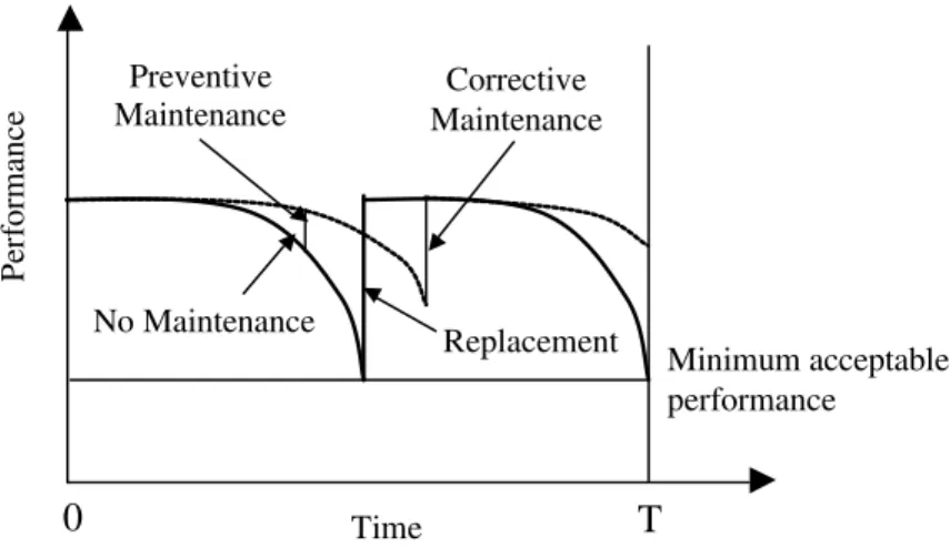
Although an accurate estimation of these costs is quite difficult, the LCC approach is efficient in comparing the long-term effects of different MR&R alternatives and in selecting the most cost-effective alternative. Figure 1 shows the life cycle performance profile of two bridges subjected to different MR&R alternatives. Although the two alternatives are acceptable technically, because they satisfy the performance requirements, the LCC approach can differentiate between the two alternatives from an economic perspective and help with the determination of the optimum alternative.

The Intermodal Surface Transportation Efficiency Act (ISTEA) recognized the importance of applying the LCC approach and stipulated a legislation that every department of transportation (DOT) in the U.S. must implement a management system for its bridge network (Czepiel 1995). A bridge management system (BMS) is defined as a rational and systematic approach to organizing and carrying out all of the activities related to the maintenance of bridges (Scherer and Glagola 1994). The major objective of a BMS is to assist bridge managers in making optimal decisions regarding the allocation of their budget to the MR&R needs of individual bridges (project level) or group of bridges (network level) based on their LCC assessment (Hudson 1987).

The final rule issued by the ISTEA in 1993 along with the guidelines of the American Association of State Highway and Transportation Officials (AASHTO) for BMSs requires that a model system should include four basic modules (AASHTO 1993): (1) a database for storing the different types of bridge data; (2) deterioration models for predicting the future condition of bridge components; (3) cost models for estimating the agency and user costs; and (4) optimization models for selecting the most cost-effective MR&R strategies at both project and network levels. These modules are organized as shown in Figure 2 according to their interaction. The arrows in this figure describe the direction of data flow among the modules. This paper focuses on bridge deterioration models since they play a key role in the life-cycle assessment of highway bridges.

A deterioration model is defined as the link between measures of the condition of a bridge and a vector of explanatory variables (Ben-Akiva and Gopinath 1995). A measure of bridge condition

in its simplest form, is a rating system that assesses the extent and severity of a specific type of damage. More complex measures can combine the extent and severity of different damage types in one rating. The explanatory variables are defined as the factors affecting bridge deterioration such as age, traffic, and weather and they can be observed or measured. Deterioration models are essential components of any BMS that predict the future condition of bridge components when various MR&R actions are implemented. The outcomes of these models along with the results of the cost models are used for the LCC assessment and the determination of optimal maintenance strategies. There are different techniques for modeling bridge deterioration, such as regression models, mathematical models, and Markov chains.

This paper presents the technique used by the state-of-the-art systems for modeling the deterioration of concrete bridge decks, and includes some examples. Further, deterioration models are developed based on data from the Ministére de Transport du Québec (MTQ), andare compared with the examples. The validation of the Markov chain assumption is investigated using a subset of the MTQ data.

DETERIORATION MODELS IN THE STATE-OF-THE-ART BMSs

Although there are several systems that comply with the ISTEA legislation, Pontis and BRIDGIT are the most popular, because of their generic design that can be adapted to accommodate the individual needs of most transportation agencies. Pontis is the predominant system employed in the United States and it is currently licensed through AASHTO to 44 users (AASHTO 1999). Pontis Version 1.01 was released in February 1992 and the latest version (Pontis 3.4.1) was released in September 1998. Pontis is a comprehensive BMS that supports functions including the collection of bridge inventory and inspection data, formulation of network-wide preservation and improvement policies for use in evaluating the needs of each bridge in a network, and the development of recommendations on the projects to be included in the agency capital plan for achieving the maximum benefit from limited funds (Golabi and Shepard 1997; Thompson et al. 1998). BRIDGIT was released by the National Cooperative Highway Research Program (NCHRP) in the fall of 1993. It is very similar to Pontis in terms of function and capabilities. The primary difference between the two systems lies in the optimization model. BRIDGIT adopted

the bottom-up approach to optimization, while Pontis uses the top-down approach (Hawk 1995; Lipkus 1994). The advantage of the former is that BRIDGIT can perform multi-year analyses and consider delaying actions on a particular bridge to a later date.

Pontis and BRIDGIT use stochastic deterioration models to predict the probability that a given bridge element in a given environment and condition state will continue to remain in its current condition state, or change to another condition state, given that a particular action is performed (Golabi and Shepard 1997; Hawk 1995). These are Markov chain models that are based on the concept of probabilistic cumulative damage, which predicts the deterioration of bridge element over multiple transition periods. Pontis and BRIDGIT use discrete parameter Markov chains, which define distinct states of bridge condition and discrete transition time intervals (Parzen 1962). The probabilities of transition from one condition state to another are represented in a matrix of order (n x n) that is called the transition probability matrix (P) where n is the number of condition states. Each element pi,j in this matrix represents the probability that the condition of

the bridge element will change from state i to state j during a certain period of time (D) called “Transition Period”. If the initial condition vector (P0) of the bridge element is known, the future

condition vector (PT) at any time (T) can be obtained as follows (Collins 1972): PT = P0 * PT/D p1,1 p1,2 ... p1,n p2,1 p2,2 ... p2,n P = . . ... . . . ... . pn,1 pn,2 ... pn,n

The transition probability matrices in Pontis and BRIDGIT are developed for the different types of bridge elements using a discrete condition rating system consisting of five states, where State 1 represents the condition of a new undamaged element and State 5 represents a severly deteriorated element. For each element type, different matrices are developed to describe the four

possible categories of environment (benign, low, moderate, and severe), and the three possible MR&R actions (do nothing, rehabilitate, and replace) (Lipkus 1994; Thompson et al. 1998).

The transition probabilities are usually obtained using an expert judgement elicitation procedure, which requires the participation of several experienced bridge engineers (Thompson and Shepard 1994). The outcome of this elicitation procedure is manipulated to generate the transition probabilities for the use by agencies with inadequate historical condition data. A statistical updating of these probabilities using the Bayesian approach can be undertaken when a statistically significant number of consistent and complete sets of condition data become available over the years (Golabi and Shepard 1997).

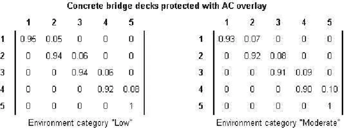
Figure 3 shows four examples of transition probability matrices for concrete bridge decks protected with “asphalt concrete (AC)” overlay and “rigid concrete” overlay in “low” and “moderate” environments when the “do nothing” option is used. These probabilities represent the change of condition of the bridge component from one state to another during a one year period under normal operation conditions excluding any emergencies, such as earthquakes, floods, fire, accidents, winds, etc. These transition probabilities are derived from the extensive literature of bridge deck deterioration and engineering judgement. The validation of these probabilities is presented in the following section using the actual condition data.

DEVELOPMENT OF MARKOV CHAIN DETERIORATION MODELS

The bridge data used for developing Markov chain deterioration models are obtained from the Ministére de Transport du Québec (MTQ) database, which is part of a comprehensive system for managing the various highway structures in Quebec. This system consists of four main modules for the identification of MR&R needs, scheduling of strategies, prioritization, and bidding. An updated version of the MTQ database is released at the beginning of each year to reflect the changes in the data that took place during the previous year. Table 1 lists some statistics on the four database versions covering the period from 1997 to 2000. According to the 2000 version, the database accounts for 9678 provincially-owned highway structures that are grouped into eight categories: culverts, slab bridges, beam bridges, box-girder bridges, truss bridges, arch bridges,

cabled bridges, and other structures. This database includes three types of data for each highway structure:

• Inventory data, consisting of approximately 220 attributes that can be categorized as: administrative data (e.g. identification, location, jurisdiction, etc.), technical data (e.g. environment, traffic, postings, etc.), and descriptive data (e.g. geometry, material, structural system, etc.) (MTQ 1997).

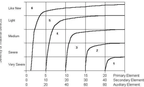
• Condition data, representing the outcome of the detailed visual inspections on approximately one-third of the structures every year. These data are collected using 21 different inspection forms, each of which corresponds to a group of correlated structural elements such as foundation elements, truss elements, and deck elements. Each inspection form includes the material condition rating (MCR), which represents the condition of an element based upon the severity and extent of observed defects, and the performance condition rating (PCR), which describes the condition of an element based upon its ability to perform its intended function in the structure (MTQ 1995). Both MCR and PCR are represented in an ordinal rating scale that ranges from 1 to 6, where 6 represents the condition of a new structure. Figure 4 shows how the MCR of an element in a highway structure in Quebec is determined given the type of element (i.e., primary, secondary, or auxiliary), percentage of the material defects in the element cross-section, surface area, or length, and the severity of these defects (i.e. very low, low, medium, severe, and very severe). Deck and wearing surfaces are examples of primary elements, sidewalks and curbs are examples of secondary elements, and drainage ditches and gutters are examples of auxiliary elements.

• MR&R data, consisting of the major maintenance actions that are recommended as future activities. The approximate cost and the expected time for each action are estimated. Data about the past maintenance activities are collected by the regional offices, each with its own practice, and not recorded in the MTQ database.

This paper focuses on concrete bridge decks, which are considered to be the weakest link in a bridge system in North America and consequently they require most of the MR&R actions. The premature corrosion of reinforcing steel as a result of using de-icing salts on bridge decks during winter, rapid degradation of concrete as a result of freezing and thawing cycles, alkali-aggregate

reaction, temperature effects, increased traffic loads, poor design and detailing, and inadequate inspection and maintenance are the main causes of deterioration in the concrete bridge decks (Lounis and Mirza 2001)

To obtain a consistent, complete, and adequate data set for developing Markov chain deterioration models for concrete bridge decks, the data records stored in the four versions of the MTQ database are accumulated in one data repository. Duplicate records are removed from this repository and the resulting data are screened by filtering out the records that do not satisfy the following requirements:

• Deck type: reinforced concrete

• Structure type: beam bridge

• Span length: greater than 6 feet

• Age: less than 100 years

• MCR: between 1 and 6

• Inspection period: between 0.5 to 5.5 years

The screening process showed 3440 beam bridges and 9181 bridge decks. Each deck consists of seven elements that are evaluated in every inspection. These elements are listed in Table 2 and are shown in Figure 5. The element weights listed in Table 2 are used to aggregate the condition of the seven elements to obtain the overall condition of the bridge deck (MCR). The MCR is equal to the weighted sum of the conditions of the two exterior faces, two end portions (each portion has a length equal to two times the girder depth), and the middle portion of the deck These weights are sometimes called “Balance Factors” and are obtained by expert judgement based on the relative importance among the various elements. Since the aggregated MCR is a cardinal number, deterioration models are developed using the MCRs of the elements (i.e. ordinal numbers) to allow the use of discrete parameter Markov chains.

Different techniques are used to develop transition probability matrices from condition data. The regression-based optimization method is the most-commonly used approach in estimating these matrices for different types of facilities, such as pavements and bridges (Bulusu and Sinha 1997). This method uses a non-linear optimization function to minimize the sum of absolute differences

1 ,..., 2 , 1 , for 1 0 : Subject to ) , ( ) ( Minimize 1 1 = = ≤ ≤ −

∑

∑

between the regression curve that best fits the condition data and the conditions predicted using the adopted Markov chain model. The objective function and the constraints of this optimization problem can be formulated as (Madanat et al. 1995):

(3)

where N = total number of facilities.

Yn (t) = expected value of facility n at age t using the regression model P = transition probability matrix.

pij = probability of transition from state i to state j.

E(tn,P) = expected condition of facility n at age t using the transition probability matrix P. k = maximum value for the bridge condition rating.

Because the regression model used in this method is affected significantly by any prior MR&R actions, whose records are not readily available in the MTQ database, the percentage prediction method is used instead. In this method, the probability pi,j of transition in bridge condition from

state i to state j can be estimated using the following equation (Jiang et al. 1988):

p

= n

/ n

where ni,j = number of transitions from state i to state j within a given time period. ni = the total number of bridges in state i before the transition.

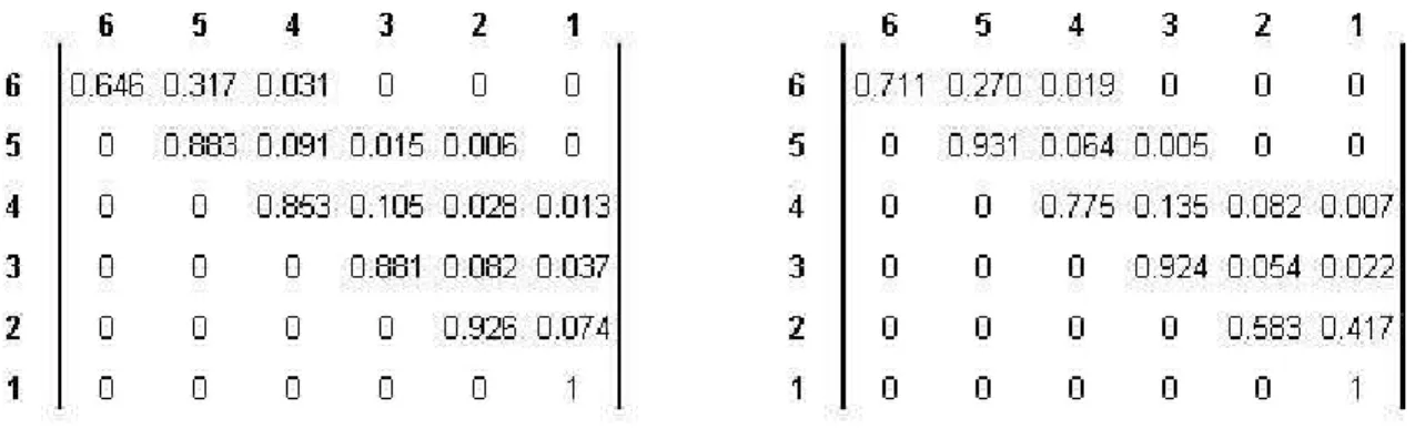
The use of this method requires at least two consecutive condition data for a large number of bridges at different condition states, which is the case for the MTQ database. Figure 6 shows the transition probability matrices developed using this method for the concrete bridge decks protected with an AC overlay and with a rigid overlay. Since the condition data used in

developing these probabilities have variable inspection periods (Figure 7), the transition period for the two matrices is considered to be 2.8 years, which is the average of the inspection periods.

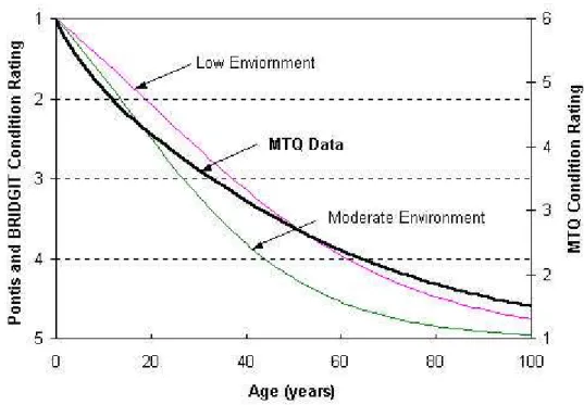
Although the transition probabilities are efficient in capturing the uncertainty and randomness of the deterioration process, these probabilities cannot be easily validated, because they cannot be compared with other probabilities developed using a dissimilar condition rating system, or a different transition period. In addition, many transportation agencies prefer to use the deterioration of a bridge element as a simple relationship between the condition of that element and its age, a deterioration curve, as reflected in Figure 1. The simple deterioration curves are easier to use and compare. Therefore, the transition probabilities adopted in Figure 3 are utilized in generating the deterioration curves plotted in light lines in Figures 8 and 9, while the transition probability matrices developed using the actual condition data (Figure 6) are utilized in generating deterioration curves plotted in heavy lines in the same figures.

Comparing the deterioration curves developed based on the literature with those developed based on “actual” condition data indicates a reasonable level of accuracy that is adequate for an analysis at the network level. However, the deterioration curves for the same element vary significantly depending on the environmental category, which requires a very precise definition of each microenvironment (e.g. humidity, snow, temperature variation, and precipitation) and operating conditions (e.g. traffic load and volume).

VALIDITY OF MARKOV CHAIN ASSUMPTION

A stochastic process is considered as a Markov process if the probability of a future state in the process given its current state, depends only on the current state and not on how the process reached it (Parzen 1962). This property can be expressed for a discrete parameter stochastic process (Xt) with a discrete state space as:

)

|

(

)

,

,...,

,

|

(

X

i

X

i

X

i

X

i

X

i

P

X

i

X

i

P

=

=

=

=

=

=

=

=

where it = the state of the process at time t

P = the conditional probability of any future event given the present and past events.

A Markov chain is a special Markov process whose development can be treated as a series of transitions between certain states. The use of Markov chains in developing bridge deterioration models is based on the assumption that the structural condition of a bridge is independent of its condition history, despite the fact that bridge deterioration is a non-stationary process (Lounis and Mirza 2001). Therefore, this assumption needs to be validated whenever facility condition data becomes available.

The validity of the Markov chain assumption was previously investigated by Madanat et al. (1997) using bridge-deck data obtained from the Indiana Bridge Inventory database. In this study, a lagged deterioration variable (a variable that represents the past condition) was incorporated as one of the explanatory variables in a random-effects model to account for the true state dependence. By examining the significance of the explanatory variables of this model, it was noted that most of the variables had become insignificant, including the age variable. This is inconvenient because it implied that it was not possible to distinguish empirically between the effects of the state dependence and the age variable in this kind of model (Madanat et al. 1997).

Another investigation of the validity of the Markov chain assumption was carried out by Scherer and Glagola (1994) using the bridge condition data obtained from the Virginia Department of Transportation. The method used in this study required at least three consecutive condition data sets that represented past, current, and future bridge conditions. The principal limitation of this method is that these data sets are not available to many transportation agencies. In this method, every two possible transition sequences that have the same current and future conditions but have different past conditions are compared to determine whether there is a significant difference in the sequence occurrences dependent on the past condition (Wirahadikusumah et al. 2001). This comparison can be achieved by either a simple frequency analysis of sequence occurrences, or an inference analysis using the chi-square statistic. The results of this investigation have concluded that the assumption of the Markov chain is reasonable for developing bridge deterioration models for network-level analysis. However, this conclusion was made for the limited data set used and

it must be verified when specific bridge components are considered and different data sets become available.

A subset of the MTQ condition data set that represents three consecutive inspection records is obtained to investigate the validity of the Markov chain assumption for concrete bridge decks using the above-mentioned method. The distribution of the number of inspection records shown in Figure 10 indicates that only about 8% of the decks have three or more inspection records, because these decks were inspected every 2.8 years on average during the period from 1993 to 2000.

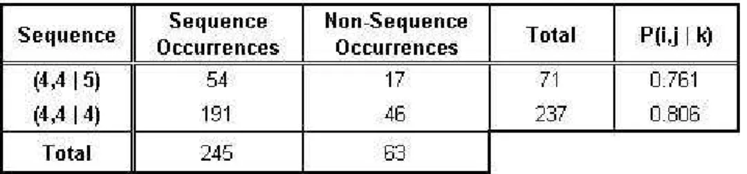
Since the available condition data do not provide adequate information about all possible condition transition sequences, only two cases of condition transition sequences are analyzed. Table 3 shows the notations and calculations used in performing the simple frequency and inference analyses for each case. In Table 3, the first column lists the two condition transition sequences being compared. Each sequence is presented in the format of (i, j | k), where i is the future condition, j is the current condition, and k is the past condition. The second column lists the number of occurrences of each sequence in the data set used along with their totals (a, c, and g). The third column lists the number of each non-sequence occurrences in the data set used along with their totals (b, d, and f). A non-sequence condition transition implies that the transition from past condition k to current condition j and then to a future condition different from i. The fourth column lists the totals of sequence and non-sequence occurrences (g and h), while the fifth column lists the probability of each sequence occurrence (m and n).

Tables 4 and 5 show comparison of the condition transition sequences of (5,5 | 6) versus (5,5 | 5), which is termed “Case 1”, and (4,4 | 5) versus (4,4 | 4), which is termed “Case 2”. In “Case 1”, 91.6% of the concrete bridge decks with a past condition equal to 6 and a current condition equal to 5, have a future condition equal to 5, while 84.3% of the concrete bridge decks with a past condition equal to 5 and a current condition equal to 5, have a future condition equal to 5. In “Case 2”, 76.1% of the concrete bridge decks with a past condition equal to 5 and a current condition equal to 4, have a future condition equal to 4, while 80.6% of the concrete bridge decks with a past condition equal to 4 and a current condition equal to 4, have a future condition equal

to 4. The difference between the two percentages of each case indicates the compliance of the case with the Markov chain assumption. The smaller the difference, the better the compliance with the assumption. Therefore, the simple frequency analysis evaluates the validity of the Markov chain assumption based on the absolute difference (? ) between the probabilities of the two condition transition sequences (m) and (n), as shown in Table 6 for the two cases. For more formal analysis, an inference testing with the null hypothesis that the generated occurrence distribution is independent of the past condition is performed. In this test, the chi-squared value (?2) is calculated using the notations of Table 3 as:

(

) (

)

and the results are shown in Table 6 for the two cases. Using a one degree of freedom (df = 1) and a significance level (a) equal to 5% results in ?2 = 3.841. This implies that there is sufficient evidence to reject the null hypothesis in “Case 1” with a 95% level of confidence, while there is inadequate evidence to reject it in “Case 2” with the same level of confidence. This indicates that the acceptance of the Markov chain assumption cannot be generalized and it needs to be verified in each individual case as long as the condition data are available.

CONCLUSIONS

This paper presents an investigation of deterioration models employed by the state-of-the art bridge management systems (BMSs). The development of reliable deterioration models is essential in the life-cycle assessment of highway bridges. The data obtained from the Ministére de Transport du Québec (MTQ) are used to develop deterioration models for concrete bridge decks using Markov chains. These models are used to validate those developed based on the literature on bridge deck deterioration and engineering judgement. This validation shows that Markov chain models are reasonably accurate for network-level analysis. It also highlights how the factors affecting the element deterioration should be incorporated in these models. A subset of the data is employed to validate the state independence assumption of the Markov chains. It is concluded that this assumption cannot be accepted in every case and it needs to be investigated for each bridge component when sufficient condition data becomes available.

ACKNOWLEDGEMENT

The authors wish to acknowledge the Natural Sciences and Engineering Research Council of Canada for financially supporting this research program, and for the Post-Doctoral Fellowship to the first author. The authors are grateful to M. Guy Richard, Eng., Director, and M. René Gagnon, Bridge Engineer, of the Structures Department - Ministére de Transport du Québec - for their invaluable help in providing the authors with all available data, manuals and other needed information.

REFERENCES

1. American Association of State Highway and Transportation Officials (AASHTO) (1999) “Pontis: The Complete Bridge Management System”, accessed on October 1999, http://aashtoware.camsys.com/html/PontisReport.html.

2. American Association of State Highway and Transportation Officials (AASHTO) (1993) “Guidelines For Bridge Management Systems”, Washington, D.C.

3. Ben-Akiva, M., and Gopinath, D. (1995) “Modeling Infrastructure Performance and User Costs”, Journal of Infrastructure Systems, ASCE, Vol. 1, No. 1, pp. 33-43.

4. Bulusu, S., and Sinha, K. C. (1997) “Comparison of Methodologies to Predict Bridge Deterioration”, Transportation Research Record, TRB, Vol. 1597, pp. 34-42.

5. Collins, L. (1972) "An Introduction To Markov Chain Analysis", CATMOG, Geo Abstracts Ltd., University of East Anglia, Norwich.

6. Czepiel, E. (1995) “Bridge Management Systems; Literature Review and Search”, [Web Page], accessed on May 1998, http://iti.acns.nwu.edu/pubs/tr11.html

7. DeStefano, P. D., and Grivas, D. A. (1998) “Method for Estimating Transition Probability in Bridge Deterioration Models”, Journal of Infrastructure Systems, ASCE, Vol. 4, No. 2, pp. 56-62.

8. Golabi, K. and Shepard, R. (1997) “Pontis: A System for Maintenance Optimization and Improvement of US Bridge Networks”, Interfaces, 27, pp. 71-88.

9. Hawk, H. (1995) “BRIDGIT Deterioration Models”, Transportation Research Record, TRB, 1490, pp. 19-22.

10. Hudson, S. W., Carmichral III, R. F., Moser, L. O., and Hudson, W. R. (1987) “Bridge Management Systems”, TRB – NCHRP, Report 300.

11. Itoh, Y., Nagata, H., Liu, C., and Nishikawa, K. (2000) “Comparative Study of Optimized and Conventional Bridges: Life Cycle Cost and Environmental Impact”, the First Workshop on Life-Cycle Cost Analysis and Design of Civil Infrastructure Systems, ASCE, D. M. Frangopol and H. Furuta (eds.), Honolulu, Hawaii, August.

12. Jiang, Y., Saito, M., and Sinha, K. C. (1988) “Bridge Performance Prediction Model Using the Markov Chain”, Transportation Research Record, TRB, Vol. 1180, pp. 25-32.

13. Lipkus, S. E. (1994) “BRIDGIT Bridge Management Software”, Transportation Research Circular, TRB, Vol. 324, pp. 43-54.

14. Lounis, Z. (1999) “A Stochastic and Multiobjective Decision Model for Bridge Maintenance Management”, Infra 99 International Congress, Montreal, Quebec, November.

15. Lounis, Z., and Mirza, M. S., (2001) “Reliability-based service life prediction of deteriorating concrete structures”, Proceedings Third International Conference on Concrete Under Severe Conditions, N. Banthia, K. Sakai, and O. E. Gjorv (eds.), University of British Columbia, Vancouver, Canada.

16. Madanat, S., Mishalani, R., and Ibrahim, W. H. W. (1995) “Estimation of Infrastructure Transition Probabilities from Condition Rating Data”, Journal of Infrastructure Systems, ASCE, Vol. 1, No. 2, pp. 120-125.

17. Madanat, S., Mishalani, R., and Ibrahim, W. H. W. (1995) “Estimation of Infrastructure Transition Probabilities from Condition Rating Data”, Journal of Infrastructure Systems, ASCE, Vol. 1, No. 2, pp. 120-125.

18. Ministére de Transport du Québec (MTQ) (1995) “Manuel d’Inspection des Structures: Evaluation des Dommages”, Bibliothèque Nationale du Québec, Gouvernement du Québec, Canada.

19. Ministére de Transport du Québec (MTQ) (1997) “Manuel de l’Usage du Système de Gestion des Structures SGS-5016”, Bibliothèque Nationale du Québec, Gouvernement du Québec, Canada.

20. Parzen, E. (1962) “Stochastic Processes” Holden Day, Inc., San Francisco, CA.

21. Scherer, W. T. and Glagola, D. M. (1994) “Markovian Models for Bridge Maintenance Management”, Journal of Transportation Engineering, ASCE, Vol. 120, No. 1, pp. 37-50. 22. Thompson, P. D. and Shepard, R. W. (1994) “Pontis”, Transportation Research Circular,

TRB, Vol. 324, pp. 35-42.

23. Thompson, P. D., Small, E. P., Johnson, M., Marshall, A. R., “The Pontis Bridge Management System”, Structural Engineering International, Vol. 4, 1998, pp.303-308. 24. Wirahadikusumah, R., Abraham, D., and Iseley, T. (2001) “Challenging Issues in Modeling

Deterioration of Combined Sewers”, Journal of Infrastructure Systems, ASCE, Vol. 7, No. 2, pp. 77-84.

Figure 2: Modules of a model BMS Optimization Models Cost Models Database Deterioration Models

Figure 1: Bridge performance with time

Time Performance 0 T No Maintenance Preventive Maintenance Corrective Maintenance Replacement Minimum acceptable performance

Table 1: Statistics from MTQ database

Table 2: Elements of the deck component and their weights Figure 4: Material condition rating system used by MTQ

Figure 7: Distribution of inspection periods in MTQ data Figure 6: Transition probability matrices based on MTQ data

Figure 9: Comparison of deterioration curves for concrete bridge decks protected with rigid overlay

Figure 8: Comparison of deterioration curves of concrete bridge decks protected with AC overlay

Figure 10: Distribution of inspection records in MTQ data

Table 3: Notations and calculations used for validation

Table 5: Comparing transition sequences for “Case 2”