An Analysis of the TR-BDF2 integration scheme
by
Sohan Dharmaraja
Submitted to the School of Engineering
in Partial Fulfillment of the Requirements for the degree of
Master of Science in Computation for Design and Optimization
at the
MASSACHUSETTS INSTITUTE OF TECHNOLOGY
September 2007
@
Massachusetts Institute of Technology 2007. All rights reserved.
Author ...
School of Engineering
July 13, 2007
Certified by ...
...
W. Gilbert Strang
Professor of Mathematics
Thesis Supervisor
Accepted by
MASSACHUSETTS INSTrTUTF OF TECHNOLOGYSEP
2 7 2007
I
\\ Jaume PeraireProfessor of Aeronautics and Astronautics
Co-Director, Computation for Design and Optimization
An Analysis of the TR-BDF2 integration scheme
by
Sohan Dharmaraja
Submitted to the School of Engineering on July 13, 2007, in partial fulfillment of the
requirements for the degree of
Master of Science in Computation for Design and Optimization
Abstract
We intend to try to better our understanding of how the combined L-stable 'Trape-zoidal Rule with the second order Backward Difference Formula' (TR-BDF2) integra-tor and the standard A-stable Trapezoidal integraintegra-tor perform on systems of coupled non-linear partial differential equations (PDEs). It was originally Professor Klaus-Jiirgen Bathe who suggested that further analysis was needed in this area. We draw attention to numerical instabilities that arise due to insufficient numerical damp-ing from the Crank-Nicolson method (which is based on the Trapezoidal rule) and demonstrate how these problems can be rectified with the TR-BDF2 scheme.
Several examples are presented, including an advection-diffusion-reaction (ADR) problem and the (chaotic) damped driven pendulum. We also briefly introduce how the ideas of splitting methods can be coupled with the TR-BDF2 scheme and applied to the ADR equation to take advantage of the excellent modern day explicit techniques to solve hyperbolic equations.
Thesis Supervisor: W. Gilbert Strang Title: Professor of Mathematics
Acknowledgments
First and foremost, I would like to thank my family. I would not be the person I am today if not for them. In many ways I was always the one who was at risk of not living up to my potential but over the years I've made strides in the right direction. So once again: thank you Mom, thank you Dad, thank you Malli for the never ceasing, never diminishing flow of comments, criticism and confidence.
Thank you to Professor Strang. Apart from teaching me how to write a thesis, he has taught me how to be a researcher. I am privileged to have worked with him and to have learned his methods. His advice on life and the personal interest he has taken in my future will always be appreciated. Thank you again sir, for taking an chance on me when I walked into your office those many months ago, looking for 'something interesting to work on'.
Finally, thank you to my friends, old and new. My time here at the Massachusetts Institute of Technology would have undoubtebly been less enjoyable if not for them. I will always look back fondly on these memories and friendships.
Contents
1 Introduction 11
1.1 M ultistep methods . . . . 13
1.1.1 Adams M ethods. . . . . 13
1.1.2 Backwards Difference Formulae (BDF) . . . . 15
1.1.3 Convergence Analysis . . . . 16
2 Nonlinear solvers 25 2.1 Newton's method for solving systems of nonlinear systems of equations 25 2.1.1 Convergence analysis . . . . 27
3 Numerical integrators 29 3.1 The concept of stiffness . . . . 29
3.2 A-stable integration methods . . . . 31
3.3 L-stable integration methods . . . . 32
3.4 Integration schemes in commercial software . . . . 36
4 Numerical Examples 39 4.1 The Chaotic Pendulum . . . . 39
4.2 The Elastic Pendulum . . . . 45
4.3 The Double Pendulum . . . . 54
4.4 The Advection-Reaction-Diffusion Equation . . . . 63
List of Figures
1-1 Adams Bashforth stability region . . . . 21
1-2 Adams-Moulton stability region for p = 1 and 2 . . . . 22
1-3 Adams Moulton stability region for p = 3, 4, 5 and 6 . . . . 23
1-4 BDF stability region for p = 1, 2 and 3 . . . . 24
1-5 BDF stability region for p = 4, 5 and 6 . . . . 24
2-1 Newton's method in ID . . . . 25
3-1 Solution to equation 3.1 with dt = 0.4 . . . . 32
3-2 TR-BDF2 stability regions . . . . 35
3-3 Magnified TR-BDF2 stability regions for y = 0.6 and -y = 2 - f2 . . 35
4-1 Free body force diagram for the simple pendulum . . . . 39
4-2 Chaotic behavior for the damped, driven pendulum with 0 = 2, o = [0.23,0.24, 0.25], F = 1.18, p= ,Wf and dt = 0.05 . . . . 42
4-3 Higher accuracy of the TR-BDF2 scheme . . . . 43
4-4 The elastic pendulum . . . . 45
4-5 Plots for 0, 0, r and i evolution with the Trapezoidal and TR-BDF2 scheme with 00 = 2, 0 = 2, ro = 1, iO = 0, dt = 0.05 . . . . 50
4-6 Plots for 6, 0, r and evolution with the Trapezoidal and TR-BDF2 scheme with 00 = 9, O = 3.5, ro = 1, iO = 0.8, dt = 0.15 . . . . 51
4-7 Plots for 0, 9, r and v evolution with the Trapezoidal and TR-BDF2 scheme with 00 = !, o = 2.5, ro = 1, tO = 0.2, dt = 0.3 . . . . 52
4-9 1 =) 2 = ,10 3 = 020= 0,dt = 0.04 . . . . 59
4-10 Poincare plots with the different methods . . . . 59
4-11 01 0 = 020 = 7,r 10 = 20 = 0, dt = 0.04 . . . . 60
4-12 Poincare plots with the different methods . . . . 60
4-13 The bacteria concentration b, using the Crank-Nicolson scheme for the diffusion subprocess of the Strang splitting. Simulation parameters: At = 0.1, Ax = 0.05, Db = 0.05, D, = 0.01 . . . . 69
4-14 The bacteria concentration b, using the TR-BDF2 scheme for the diffu-sion subprocess of the Strang splitting. Simulation parameters: At = 0.1, Ax = 0.05, Db = 0.05, D, = 0.01 . . . . 71
Chapter 1
Introduction
In the context of ordinary differential equations (ODEs) the trapezoidal rule is a pop-ular method of choice and has already been implemented in the well known circuit
simulator SPICE [1]. However, it is well known that for extremely stiff problems this
method is not efficient: the stability regioni of the trapezoidal rule forces a drastic reduction in the maximum allowable time step in order to compute a numerical
solu-tion. What makes things especially tricky is that the majority of nonlinear dynamics
problems can transition between being stiff and non-stiff. It would be ideal to have a method of numerical integration that would encapsulate the ease of implementation of the trapezoidal rule as well as second order accuracy, while not having to worry about our nonlinear system becoming excessively stiff.
The method we study is in some sense a cyclic linear multistep method, consisting of an initial step of the Trapezoidal rule, followed by a second order backward differ-entiation formula. This method is more commonly known as the TR-BDF2 scheme
(originally devised by Bank et al [2]) and is second order accurate. More importantly, it is L-stable (explained in section 3.3). This combination has a significant advantage
over the Trapezoidal rule alone (which will be shown to be only A-stable) when it 'The stability region of a numerical method is defined to be the values of z = Aih (possibly
complex) which ensure that the amplification factor of numerical errors in our solution is strictly less than one. Here, A2 are the eigenvalues of the Jacobian of our differential operator and h is the
comes to numerical damping of oscillations in our solution.
We begin this thesis by familiarizing ourselves with some well established concepts. We first introduce the notion of a multistep method, after which we elaborate on the nonlinear solver (Newton-Raphson) that we use throughout our analysis. Then we explain how these two ideas together can be used to integrate systems of differential equations. We proceed to define exactly what it means for a method to A-stable and L-stable and the implications and possible hazards of the former.
The section on numerical results is intended to highlight one of the key points made throughout this thesis: the numerical damping provided by widely accepted integration methods (Crank-Nicolson and the Trapezoidal rule, which are both only A-stable) is insufficient in extremely stiff systems. We apply the TR-BDF2 and Trapezoidal integrators to a wide range of problems arising in nonlinear dynamics. The systems we considered were primarily pendulum examples (chaotic, double and elastic). We end by briefly touching on how the idea of operator splitting can be used to very efficiently solve a coupled system of partial differential equations (PDEs)
-namely the advection-diffusion-reaction equation, by applying a different integration method to each subprocess.
1.1
Multistep methods
1.1.1
Adams Methods
It is standard practice when faced with a partial differential equation involving space and time, to first discretize the spatial variable(s). After this initial discretiza-tion (more formally, a semi-discretizadiscretiza-tion) we are left with an initial value problem for a set of ordinary differential equations. ODEs arise as a result of Fourier analysis and splitting methods, when applied to PDEs. The focus of this thesis will be mainly on linear multistep methods, which are powerful techniques to solve ODEs approxi-mately. Runge-Kutta algorithms and Adams methods are perhaps the most popular choices, however we will be focusing on the Adams schemes.
The least accurate Adams schemes are the Forward and Backward Euler algorithms (which are single step methods). The idea behind these multistep methods is that we may better approximate the local gradient by taking into account an increasing number of previous/future values of the function to be integrated. For example, consider solving the ordinary differential equation
dy =
(1.1)
dt
We can step forward in time by calculating
Yn+1 = yn + f (y, t) dt (1.2)
The Adams family of multistep methods is derived by computing the integrand approximately, via an interpolating polynomial through previously computed values of the function
f
For example, consider using the value of fn and fr_1 to interpolate our functionf
and hence compute the integrand. Definet - tn ________1
P(t) =
f
(yn-, tn1) - + f (yn, tn) - (1.3)Assuming that we have a uniform discretization with stepsize h, say, our integrand becomes
/tn+1
tn f (y7t) dt j~ P(t) dt n+1 t - tn t - t = f (ynt) h , i ) htf dt h fy, t -1 2 tn+1 -h t - n ]2n+1 2 y h tn 2 h tn h = [3f (yn, tn) - f(yn_1, n_1)] (1.4) (1.5) (1.6) (1.7)So finally we are left with an explicit expression for Yn+1
h
Yn+1 = Yn + - [3f(y., t.) - f (yn1, itn 1)]
2 (1.8)
Explicit schemes of this kind are known as Adams-Bashforth methods. In general, an nth order scheme can be expressed as
n
Yn±1 = Yn +
Swif
(Yn~lpi, tn+l1 i) (1.9)It is clear why these methods are coined as explicit: when we know the values of our function
f
at the required stages of the method, we can directly calculate the value of Yn+1. This is not the the case for an implicit method where we will be required to solve an equation to obtain the value of our next iterate,Yn+1-It is straightforward to calculate the next few expressions for increasingly higher order approximations. For completeness we list them here up to third order (the first order Adams-Bashforth method is more commonly known as the Forward Euler method).
Yn+1 = yn + hf (y, tn) (1.10)
h
Yn+1 = Yn + - [3f (yn, tn) - f (yn 1,i)] (1.11) h
Yn+1 = yn + 11 [23f (yn , n) - 16f (yn_1, tn_1 + 5f (yn- 2, tn- 2)] (1.12)
For the implicit Adams methods (more commonly known as the Adams-Moulton methods) there is one additional term in the multistep equation:
n
Yn+1 = Yn + wOf (Yn+l, tn+1) + wif (yn+l-i, tn+l-i) (1.13)
Note now that since Yn+i appears on both sides of 1.13 we need to solve this equation for yn+i (hence the term implicit). If the function
f
is nonlinear, a nonlinear solver such as Newton-Raphson may be required.Once again, with the same technique as above (using an interpolating polynomial to approximate our integrand) it is trivial to calculate the weights wi for these implicit schemes. The first, second and third order Adams-Moulton methods are listed below:
Yn+1 = yn + hf(yn+i, tn+1) (1.14)
Yn+1 = Yn + h [f (yn+1, tn+1) + f (yn, itn)] (1.15)
h
Yn+1 = Yn + h [5f(yn+1,
tn+1)
+ 8f (ynt n) - f (yn_1, tn_1)] (1.16)The first order Adams-Moulton method is more commonly known as the Backward
Euler while the second is known as the Trapezoidal rule.
1.1.2
Backwards Difference Formulae (BDF)
We derived the Adams methods described earlier by approximating the derivative
integrated to get the value of yn+1
In Backwards Differentiation methods, we approximate y' = f(y, t) at t = t,+1
using a backwards differencing formula. For example,
Yn+ Yn f (n+l, n+) (1.17)
h
We recognize this as the Backward Euler formula from earlier (the first order Adams Moulton method).
We can increase the order of our BDF by taking into consideration more terms:
3 1
~yn+1 - 2yn. + g yn-i = hf (yn+1, tn+1) (1.18)
-Yn+1 - 3yn + -Yn-1 3Yn 2 =hf (yn+1, tn+1) (1-19)
We will see later on that BDF have an important role in solving stiff systems of differential equations. Loosely speaking, the term stiff means that the step size for the approximate solution is more severely limited by stability of the method of choice than by the accuracy of the method. This is explained in greater detail in section
3.1. Stability and accuracy are defined later in this chapter.
Backwards differentiation formulae are implicit, like the Adams-Moulton methods. In practice they are more stable than the Adams-Moulton schemes of the same order but less accurate. It also worth noting that BDF schemes of order greater than 6 are unstable [5].
1.1.3
Convergence Analysis
To recap, the goal is to solve the initial value problem
y= f(y, t), a < t K b
y(a) =a
We have our multistep method
Yn+1 = yn + Wif (yn+1-i, tn+1-i) (1.20)
i=O
where w(0) could possibly be zero, depending on whether or not we are using an implicit scheme.
Then, given a stepsize h we say that a multistep method is convergent if we can achieve arbitrary accuracy with a sufficiently small h, i.e.
lim yN - y(tn)I = 0
h-+O
With the goal of understanding convergence, we define the global error e,
en = yn - y(n) (1.21)
where yn is the approximate solution for y (from our multistep method) and y(tn) is the exact solution for y at time t = tn. A natural question then is: how does the
global error en behave? Does it tend to zero as our stepsize h tends to zero?
Before we begin to address these questions, it is useful to define the notion of order
of accuracy of a multistep method. We first define the local truncation error (LTE)
assuming that the previously computed value of y, was identically equal to the exact solution for y at time t = t,. We then say that the multistep method is of order p if
1
n+1 = O(hP+l)
For example, consider the previously derived expression for the Adams-Moulton second order method, (the Trapezoidal rule) equation 1.16
h
Yn+1 = Yn + h [f(yn+l, tn+1) + f(yn, tn)]
Then, our definition of the LTE yields
In+1
= y(tn) +h[f(yn+
1,t
n+1) + f(ynt n)] - y(tn+l)h
= y(n) + - [y'(tn+1) + y'(tn)] - y(tn+l)
2
(1.23) (1.24)
We can combine y(tn+l) and y'(tn-i) by Taylor expanding about t = tn
Y(tn+l) = y(tn) + hy'(tn) +
h-Y"(tn)
+ 0(h0)2
y'(tn+1) = y'(tn) + hy"(tn) + O(h2)
Substituting all this into the expression for the LTE:
(1.25) (1.26)
1n+1 = y(t7n) +
h
h [y'(t) + hy"(t) + O(h2)+ y'(tn)] -
fy(tn)
+ hy'(tn) += 0(h3)
By definition, the Trapezoidal rule is indeed second order accurate. So now, with the goal of quantifying the global error we define the notion of stability for a multistep method
+ O(h3)]
Yn+1 Yn + Ein+-i + h n-j (1.27)
j=z-1
We associate with each multistep scheme the characteristic polynomials
(1.28) (1.29)
0-(rI) = Or + Or-ir1 + 3r-2A72 + ... +
i-i±r+1
(Note that for all of the Adams' methods, ai = 0)
We then say that the root condition of the multistep method is satisfied if the roots of p( ) = 0 lie on or inside the unit circle. If this condition holds, our multistep method is stable.
We say the method is consistent if
p(1) = 0
p'(0) = -(1)
Then, we can finally say our multistep method is convergent if and only if the root condition is satisfied and the method is consistent.
The proof of this result is somewhat lengthy and the reader can refer to
[3].
It is also common to define the notion of strong and weak stability. The method is considered to be strongly stable if = 1 is a simple root and weakly stable otherwise.After establishing the stability of the multistep method, we now need to determine the allowable step-sizes with which we can march forward in time. More precisely,
i=1
given our computed approximate solution ya, which satisfies our multistep equation, does the method allow perturbations
yn= yn + en
to grow. That is, does lim_.oo leni = o0?
Consider for example the Forward Euler algorithm. For simplicity, assume now that f(y, t) = Ay + f(t) in equation 1.2. Then the multistep equation reads:
Yn+ =?in +f(ta)
h -An+f(n
Yn+1 + en+1 - yn - en
h = A(yn + e,) + f(tn)
Now we know that y satisfies the exact multistep equation. That is:
Yn+1 - yn= A(y) + f(t) h
So we are left with:
e±n+ - en
h = e
= en+1= (1 + Ah)en
So en satisfies the homogeneous difference equation. We now introduce an
ampli-fication factor g (1.33) en+1 = gen (1.30) (1.31) (1.32)
Thus if Ig| > 1 then limn-o, lenl = oG.
Calculating g for the Forward Euler discretization yields: g = 1 + Ah. It is then common to visualize the values of A and the stepsize h on the complex plane which ensure that
IgI
< 1. We set z = Ah and denote this set of allowable values the stabilityregion for the Forward Euler method.
For comparison, the stability regions for p = 2, and p = 3 are also plotted.
1.5
1
0.5
-0
Adams-Bashforth stability regions in the complex plane
-0.51--1
-1.51
-2 -1.5 -1 -0.5 0 0.5
Figure 1-1: Adams Bashforth stability region
I I I I I
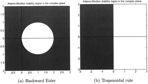
Adams-Moulton stability region in the complex plane Adams-Moulton stability region in the complex plane
-1 -u.3 u u.3 I I.U z
(a) Backward Euler
-2 -1 0 1 2 3
(b) Trapezoidal rule Figure 1-2: Adams-Moulton stability region for p = 1 and 2
We can just as easily derive the stability region for the Adams Moulton methods using the same method as before: Taylor expand to obtain the amplification factor g, then plot the values of z which ensure
IgI
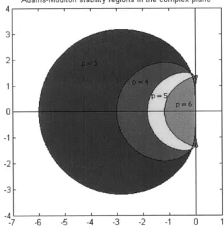
< 1 on the complex plane.4 3- 21 - 0--1 --2 3 --4 -7
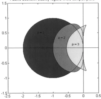
Adams-Moulton stability regions in the complex plane
-6 -5 -4 -3 -2 -1 0 1
Figure 1-3: Adams Moulton stability region for p = 3, 4, 5 and 6
a
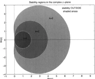
Similarly, we have the stability regions for the Backwards Differentiation Formulae derived earlier: 4 3 2 1 -1 -2 -3 -4I -1 0 1 2
Stability regions in the complex z-plane
stability OUTSIDE
"A shaded areas
3 4
Re(z)
5 6 7 8 9
Figure 1-4: BDF stability region for p = 1, 2 and 3
Stability regions in the complex z-plane
stabirity OUTSIDE shaded areas
5 10 15 20 25 30 35
Re(z)
Figure 1-5: BDF stability region for p = 4, 5 and 6 15 10 5 0 -6 -15--10 -5 0
Chapter 2
Nonlinear solvers
2.1
Newton's method for solving systems of
non-linear systems of equations
Newton's method (or the Newton-Raphson method) is a well known iterative nu-merical technique for finding the (real) roots of a function
f,
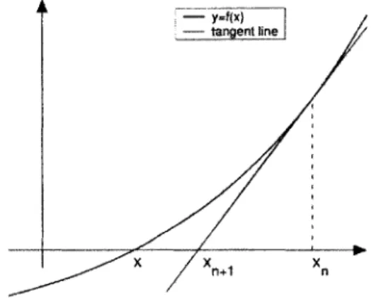
say. We will see that it is a very efficient root finding algorithm, in the sense that if our current iterate is 'close' to a root, we will converge quadratically to it.- tangetln
Xn+1 X
Figure 2-1: Newton's method in ID
Newton's method is perhaps most easily explained with an illustration in one di-mension. The idea is simple: at each iterate x, we draw the tangent to the function
and calculate where the tangent line intersects the x-axis. We take this value of x as
our new iterate, xn+1
-Mathematically speaking:
f '(Xn) 0 - f(xn)
Xn+1 - Xn
Rearranging this equation for our new iterate we obtain:
Xn
Xn+1 = Xn - f (X) (2.1)
The idea of root solving in this way extends naturally to higher dimensions. Assume now that we are to solve n nonlinear equations. We can write these n equations as:
f(_X) = 0
where x is an n dimensional vector and
f
: Rn -* RProceeding in the analogous way as the one dimensional case, we replace the scalar derivative f'(xn) with a matrix of derivatives called the Jacobian.
'x1
J= ... 211
/9f
We can demonstrate the method with an example: consider solving the system of equations with two unknowns
f,(x, y) = xy2 + sin(y) = 0
Our Jacobian matrix is then a_[ f J(x, y) a x af2 X-D22 2 j-- -sin(x) 2xy + cos(y) 3y2
So the Newton-Raphson iterates are as follows:
[
-n+1 n _1 f1(X, yin)Yn+1 Yn
J
[
f2(X, yn)substituting our expressions iterative algorithm:
[
Xn+1F
1
Yn+1 L n I
for J, fi(x,, y,) and f2(x,, yn) to give us the explicit
[
yn2
-sin(Xn) 2xyn + COS(yn) 3y -1 2 Xnyl + sin(yn) cos(x) + y3 n zn yn Residualf1 Residualf21 6.863161e-001 3.985806e-001 1.841471e+000 1.540302e+000 2 1.672218e+000 -4.654934e-002 4.971432e-001 8.369068e-001
3 1.570680e+000 4.597843e-003 4.290910e-002 1.013492e-001 4 1.570796e+000 3.269765e-005 4.63103le-003 1. 164770e-004 5 1.570796e+000 1.679210e-009 3.269933e-005 1.923241e-007 6 1.570796e+000 4.429249e-018 1.679210e-009 7.000528e-014 7 1.570796e+000 0.00000000000 4.429249e-018 6.123234e-017
2.1.1
Convergence analysis
An attractive feature of the Newton-Raphson method for solving systems of equations is that we can obtain quadratic convergence under certain assumptions (discussed at the end of this section) once we are sufficiently close to the solution. We briefly present the proof of this for the one dimensional case.
I
Assume the equation we wish to solve is f(x) = 0 with corresponding solution
x = x*. Then we can truncate the Taylor expansion about our current iterate 1 k at
the point x* using the mean value theorem to yield
f (xk) + df(xk)(x* - Xk) + 1 d2
f
2 dx2(x)(x - xk)2
for some r E [xk, x*]
We then truncate the Taylor expansion about the solution Xk at our next iterate,
Xk+1
0 = f(xk) +
dj
(Xk)(Xk+1 - Xk) (2.3)Subtracting we obtain
df (Xk)(Xkd d 2f
(xf)(xk+1 - Xk) = dx2 (z)(x* - xk)2
If we assume that [ (x)] {(x) < L Vx we then have
|Xk+1 - xl < Ljxk -
x*|2
Hence we see quadratic convergence if L is bounded.
(2.4)
(2.5)
Chapter 3
Numerical integrators
3.1
The concept of stiffness
Stiffness is a phenomenon exhibited by certain ODEs. Physically, it signifies the fact that the solution has constituents which independently evolve on widely varying time-scales. We can elucidate this point with a concrete example. Consider the equation
y" + lOy' + 99y = 0 (3.1)
The eigenvalues are A, = -99 and A2 = -1, so the solution is given by
y = Ae-t + Be~99t (3.2)
Now, one would expect to be able to 'ignore' the transient Be- 99t term when it
becomes 'insignificant' but stability theory dictates that we need our step length h, multiplied by our largest negative eigenvalue A, to lie in our absolute stability region (as discussed in section 1.1.3). Should we use Forward Euler, this would restrict our
choice of h to lie in the range
2
0 < h <
Needless to say, this is a very severe constraint on our maximum allowable stepsize in order to guarantee stability. More often than not, to bound the LTE (and hence maintain a desired level of accuracy) when calculating a numerical solution, the step length predicted to meet these requirements is safely within the stability region. However, there are instances (as seen in example 3.1) that this is not the case - the maximum possible step length is determined by the boundary of the stability region.
Problems with this feature are classified as stiff.
Mathematically, we can also say the ODE
y' =
f
(t, y)is stiff if the eigenvalues of the Jacobian differ in magnitude by a significant amount. What this practically means, is that if an explicit method is used (such as Forward
Euler) to meet stability requirements we have to use an extremely small step size h
to march the solution y in time. It seems computationally inefficient to be doing so many steps to compute our numerical solution, which we already may know to be reasonably smooth.
3.2
A-stable integration methods
The notion of stability as motivated by Dahlquist has a strong connection with the linear model problem:
y= Ay (3.4)
where A is a complex constant with a negative real part.
We say that a numerical method is A-stable if its stability region contains the whole left half plane. This is a very strict requirement: we can immediately deduce that explicit methods (which have finite stability regions) cannot meet this criterion. For example, all of the explicit Runge-Kutta (RK) methods have finite stability regions'
It is easy to see that the trapezoidal rule is indeed A-stable. For our model problem, we have
I1+ MhA
yn+1 1 - !hA y (3.5)
2
and for stability, 1+-hX < 1 e Re(hA)< 0. Therefore the trapezoidal rule is
1 2
A-stable. It is straightforward to show that Backward Euler is also A-stable.
The trade-off in using an implicit method, which can guarantee A-stability at each iteration, is that we must solve a system of (possibly nonlinear) equations. The Newton-Raphson method is usually the method of choice because more often than not (provided we are using a reasonable step size h) we have a good initial guess, so
quadratic convergence is observed almost immediately.
In the context of the linear model problem above: we know the system is stable for all Re(A) < 0. Given this, it would be nice then, if our integration method was stable
for any step length h, i.e. our stability region should be the entire left half plane
-hence an A-stable integration method.
We will see later on, that for the nonlinear examples we consider, although A-stable methods can be used, they come with an important caveat: sometimes these integration methods do not provide adequate damping to maintain stability (in par-ticular, the dynamical systems that exhibit chaotic behavior). Round-off errors can
accumulate to the point where they cause our numerical solution to explode.
3.3
L-stable integration methods
As briefly motivated at the end of the last section, A-stable methods must be used with caution. We proceed to define what it means for an integration method to be L-stable and highlight examples of where A-L-stable methods fail to produce a numerical solution while L-stable methods do not break down.
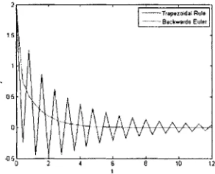
Beneath is the solution to (stiff) equation 3.1 with the initial conditions chosen to ensure that A = B = 1 using the second order Trapezoidal rule and the first order Backward Euler method. The fact that the Trapezoidal rule is only A-stable manifests itself as the 'ringing' effect seen below.
Ft
NVV0A
5150
12
L-stability is a stronger requirement than A-stability. Once again, its definition is based on the linear test problem y' = Ay. We say that the integration method is L-stable if yni+/Yn -- 0 as hA -+ -oo
We now show the trapezoidal rule (proven earlier to be A-stable) is not L-stable. We know Yn+1 1+ !hAY2 (3.6) y1 - jIhA2 1 + hRe(A) + 1h 2JA 2 1- 1 as hA -+ -oo (3.7) 1 -hRe(A) + -12 A21
There is however a way to overcome this difficulty using a extrapolation/smoothing technique [7] but that is not the focus of this thesis.
The L-stable method which we will be focusing on will be the composite second order trapezoidal rule/backward differentiation method (TR-BDF2). For simplicity, assume we already have a second order accurate discretization of the form
dy - (y) =
Ay dt
Then, as intuition might suggest, the TR-BDF2 scheme consists of two steps: the first marches our solution from tn to t,+, using the (second order) Trapezoidal rule
-At At
yn+, - 2y-Ayn+, = yn + -y-Ayn (3.8)
2 2
and the second step marches our solution from tn+, to tn+1 using the second order Backward Differentiation Formula (BDF2)
I - Y 1 (1 -- Y)2
Yn+i - AtAyn+1 Yn+-Y y(3.9)
It is worth noting that the Jacobians for the Trapezoidal rule and the BDF scheme are: At JTrap = I - A 2 JBDF =-I AtA 2 -y7
These matrices are identical if
2 2 -y
-Y 1-7
Solving this gives -y = 2 - v/5. Using this value of -y means the Jacobian matrices for the Trapezoidal and BDF steps are the same. This means we only have to invert one matrix for the TR-BDF2 method, even though we are using two different implicit schemes. It was also proven that it is precisely this value that minimizes the LTE when implementing the TR-BDF2 scheme [2].
We now proceed to prove that the TR-BDF2 scheme as described above with this value of -y is indeed L-stable. From the Trapezoidal step, we have
=(2 - yhA)
Yn+y (2yhA)9n (3.10)
(2 + 7hA)
Substituting this into the BDF2 formulae, we have
=1 (2 -yhA) _(1 - 7)2
(2- - )yn+ -(I - )hAyn+1 - n - 1__/2n (3.11)
-y (2 + -yhA) 7
Setting z = Ah we can simplify this expression for yf+1
2(2-7) - z(1 + (1 - _) 2)
z2 Q - 1)y + z(-y2 + 4y - 2) + 2(2-'y) y, (3.12)
(3.13) 2(2 - -) z(1 + (I_ - y)2)
z2(-y _ 1)- + z(-7 2 + 4-y - 2) + 2(2 - -y)
and this clearly tends to zero, as IzI -+ oc. By definition then, the TR-BDF2 scheme is L-stable. We can plot the stability regions (which are outside the bounded areas) for different values of the parameter -y. We see that when -y = 1, we are essentially using the Trapezoidal scheme, hence our stability region is the left-half plane.
TR-60F2 stability regions
10 -
---5 0 5 10 15 20 25
Figure 3-2: TR-BDF2 stability regions
TR-BDF2 stability regions 0 0 6- - -- -.. -- -... --- . . .-004 - -- - -00 -0 0 4 -. -. -. - -.---.-.-.--. .. . . -0'0 2 162 11.64 11,66 11 60 11.7 1172 11.74 11.76 Real
3.4
Integration schemes in commercial software
Given the numerous integration schemes that exist today, a natural question might be "which method(s) are actually being implemented in commercial software applica-tions?" to solve ODE's which arise in industrial settings. Companies which specialize in circuit and structural analysis simulators clearly need accurate, robust solvers which will produce results in an acceptable amount of time. We briefly look at some
of the industry-standard codes and which integration schemes they employ.
ADINA2 (Automatic Dynamic Incremental Nonlinear Analysis) is one of the lead-ing finite element analysis products available. It was founded in 1986 by Dr. Klaus-Jiirgen Bathe, a professor at the Massachusetts Institute of Technology. Their soft-ware is currently being used for many applications [8]: at the California Department of Transportation in the design and testing of bridges for seismic analysis. ACE Controls, which manufactures shock absorbers (where linear deceleration is critical) for the automotive industry and theme parks chose ADINA from eleven other soft-ware providers. ADINA gives the user the option of using the TR-BDF2 integration scheme to solve fluid-structure, fluid flow and structural problems.
PISCES is another well known commercial piece of software, developed and main-tained by the Integrated Circuits Laboratory at Stanford University. PISCES is a device modeling program which predicts component behavior in electrical circuits and is widely regarded [9] as "the industrial device simulator standard". Simucad, Synopsys and Crosslight sell commercial versions of the code which are used in the manufacturing process of integrated circuits as well as the perturbation analysis of individual components. Currently, six of the top ten electronics manufacturers [10] use code from Crosslight Software Inc.
PISCES gives the user the option of using either the TR-BDF2 scheme or the Backward Euler method. However the stepsize used is calculated automatically by
2
The ADINA programs are developed in their entirety at ADINA R & D, Inc. and are the exclusive property of ADINA R & D, Inc.
the software and is dynamically adjusted during the simulation.
One might ask why we persistently use backwards differentiation schemes, given their natural dissipativeness. There are several reasons for this, the first being that these methods greatly reduce the number of functions evaluations required to compute a numerical solution. In [4], Gear describes in great detail the expense of these operations in circuit simulation. Secondly, we can very easily implement a higher order method without much extra cost.
The trapezoidal rule is not considered suitable for these applications because of its lack of damping. Since the trapezoidal rule conserves energy, oscillations are not damped at all (even the very high frequency ones which result from numerical noise) so errors propagate without being damped (see Figure 3.1). It is with this in mind that the TR-BDF2 scheme was constructed. With it, we can combine the advantages of each method: the energy conservation property of the trapezoidal rule as well as the damping properties of our backwards differentiation scheme.
Chapter 4
Numerical Examples
4.1
The Chaotic Pendulum
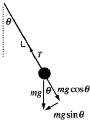
L
6m09 Mg cos6
mgsin6
Figure 4-1: Free body force diagram for the simple pendulum
Throughout history, pendulums have had an exclusive role in the study of classical mechanics. In 1656, Christiaan Huygens invented the first pendulum clock which kept
time accurately to an error of 10 seconds a day. In 1851, Jean Foucault used it to provide proof that the earth was rotating beneath us. Even today, pendulums serve as prime examples in the study of nonlinear (including chaotic) dynamics because of their natural oscillatory nature.
Under certain conditions, (namely a driving and damping force) we can make the simple pendulum exhibit chaotic behavior. By 'chaotic' we mean extreme sensitivity to initial conditions: the slightest of changes in how the system was initially configured can lead to large deviations in the long-term behavior of the system. The chaotic pendulum is an example of 'deterministic chaos' - meaning that at all times of the motion Newton's laws are obeyed. There is no randomness or stochastic element to the problem.
We begin by deriving the equation of motion for the damped, driven pendulum. When gravity is the only force present, the pendulum obeys
-mgl sin(9) = m129 (4.1)
where 0 is the angular displacement from the horizontal.
We then add a damping force m103 and a periodic driving force mlCsin(wjt), so our equation of motion becomes
1 -/ C
-O + -0 + sin(O) = -sin(wft) (4.2)
9 9 9
We then rescale time by setting t = s 9. Finally we are left with
0 + PW + sin(9) = Fsin(#) (4.3)
To apply our integration methods we write this as 3 first order differential equa-tions:
(4.4)
C = -puw - sinO + Fsin() (4.5)
Here p is the coefficient of damping and g is the amplitude of the (periodic) forcing. We now apply our usual trapezoidal step:
Att +-t
'A At
wt+. - t -Iwt+! - sin±i. + F sin( ±t+.) = wt + - t - sinOt + Fsin($t) (4.8)
At At
Owl - t W = t + tWf b (4.9)
The Jacobian matrix, J is now found by taking partial derivatives of this nonlinear equation as described in the earlier section:
2 -At 0
J A t cos() 2 + pAt -AtFcos(#) (4.10)
0 0 2
We use the scheme as above for the pure Trapezoidal scheme. For the TR-BDF2 method, we then use a 3 point backward Euler BDF2 step (given below) to evaluate the first derivative (which is the same operation for each unknown, U). The Jacobian for the BDF2 step (although a little more tedious) can be similarly derived.
1 4 3
&t+1 = 1 Ut At Ut+ + At Ut+1 (4.11)
Fortunately from the result in Section 3.3 we know we do not need to calculate the Jacobian matrix for the BDF2 step: by setting -y = 2 - v/2 we ensure both matrices are the same, saving us an extra calculation.
In this section, with the intention of demonstrating the importance of choosing an appropriate numerical integration technique, we present the results of applying the Trapezoidal rule and the TR-BDF2 integration scheme to the chaotic (damped, driven) pendulum. Solutions were computed over an interval of 40 seconds. At each iteration, the coupled nonlinear equations were solved using the Newton-Raphson method to an accuracy of 10-8.
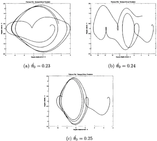
The parameters selected for the following examples were intentionally chosen to lie in the chaotic regime of the motion. Note the Poincare plots for the pendulum, when the initial velocity is perturbed in increments of 0.01
-2 ~ 1.
(a) 0o = 0.23 (b) do = 0.24
I(
(c) do =0.25
Figure 4-2: Chaotic behavior for the damped, driven pendulum with 60 =
2, o =
We now demonstrate the superior performance of the TR-BDF2 scheme over that of the Trapezoidal scheme for the
I. 18, )
12 -1
.,$ 2 1j -2 -,
(a) Trapezoidal rule dt 0 07
//l
(..5 r0
-2 1
-12 .1 - -2 2
12 R r
(e) Trapezoidal rule dt = 0.03
last example given (Oo = , 0o = 0.25, F
2/ (b) Trapezoidal rule dt 0.06 2 -/N J (d) (f) -1 8-2 0 2 Trapezoidal rule dt = 0.04 } -Trapezoidal ruledt = 0.02
A theoretical stability analysis of the model we have used for the chaotic pen-dulum would be very difficult to carry out because of the nonlinear nature of the coupled equations. Therefore we have to draw conclusions based on the results of our numerical simulation, since we cannot solve the model analytically.
Figure 4-3 is a very insightful one: with a stepsize of dt = 0.05 using the TR-BDF2 scheme, the numerical solution obtained is almost identical to that of the Trapezoidal scheme with a stepsize of dt = 0.02.
Several parameters were experimented with (F, p, wf, dt as well as 00 and O) but
it proved difficult to find a parameter set which exposed the numerical instability of the Trapezoidal scheme (see Section 3.3). However our next example, the elastic pendulum, gives some compelling evidence to warrant our claim that purely A-stable methods should be implemented with caution: not just on the ground of 'greater accuracy', but based on the fact that they are genuinely more stable.
An animated movie of the chaotic pendulum with these parameters is available
online from http: //www-math.mit .edu/18085/ChaoticPendulum.html for both the
Trapezoidal and the TR-BDF2 scheme. It can be seen that when the r and the 0 components were too high (relative to the selected time step) the numerical solution from the Trapezoidal rule blew up.
4.2
The Elastic Pendulum
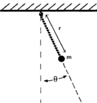
The elastic pendulum is another model problem for us to use the ideas of numerical time stepping to predict evolution. The elastic pendulum, as the name might suggest is modeled as a heavy bob of mass m attached to a light elastic rod of length r and modulus of elasticity k which is allowed to stretch, but not bend. The system is free to oscillate in the vertical plane.
m
Figure 4-4: The elastic pendulum
Since the equations of motion are not as well known as the simple (inelastic) pen-dulum, we will derive them from Lagrange's equations. We begin by constructing the Lagrangian. The kinetic energy T is the sum of the transverse and radial kinetic energies of the bob:
T = (W + r2 ) (4.12)
2
The potential energy, V is the sum of the elastic potential energy in the rod and the gravitational potential energy of the bob:
V = k(r - L)2 - mgrcosO (4.13)
So our Lagrangian L is then defined as T - V
L = $( + r202) - k(r - L + mgrcosO (4.14)
The equations of motion are exactly the Euler-Lagrange equations
dOBL DL
- ( - O =L _0 (4 .1 5 )
dt O<) aq
where q and e4 are the state variables r and 0 and their derivatives, respectively.
Hence the governing equations are:
k
= gcosO - --(r - L) + r02 (4.16)
2M + gsiri9
(4.17)
-r
Linear analysis of this problem is very straightforward: we can integrate the gov-erning equations of motion exactly using analytical techniques. However, this comes at a price because it is only when nonlinear effects are taken into account that we can accurately capture the coupling effects between the elastic oscillations in the rod and the rotational motion. We will see that solving the resulting (coupled) nonlinear equations has to be done numerically with an appropriate scheme (explicit methods are notoriously inefficient at solving systems of stiff nonlinear differential equations
-see equation 3.1).
As described earlier, the trapezoidal rule can be used to time integration when we have a first order ordinary differential equation: hence we introduce new variables
R=r (4.18)
E=o
(4.19)0 r R 0 2te+gsinO -r R gcosO - '{r - L) + rO2
Now this is exactly in the form we require to use our trapezoidal integrator: comparing the above equation with an ODE in standard form:
dx
- = f(x,t)
dt
So substituting into the trapezoidal rule:
dt
- 1(f'(xn, t) + f'(Xn+1, tn+1))and using subscripts to denote the time at which we evaluate each term, we end up with:
At 2
We observe that now our variable x is identical to our state vector, U and f(x, t) plays the role of our derivative vector, V.
0 E r R and
e
2t9+gsinO -r R gcos - (r - L) + rE2What remains now is to illustrate how we use the Newton-Raphson process to solve this implicit equation for our new state vector, Ut+1.
At Rt+1 - - gcosvt+1 2 ( Ot+1 - -- Et+1 2 - t (2Rt+1E 1+1 +gsin0t+ 1 2 -rt+i At rt+i - t+1 2 k k (rt+1 m - L) + rt+1E)+1) At = rt + -t 2 = t+At 2 Rt0t + -_sin0t. 2 -'rt = rt + 2Rt = ~±At
(
Rt + Atgcoso 2 ( k mThe Jacobian matrix, J is again found by taking partial derivatives of these non-linear equations as described in the chapter on nonnon-linear solvers, Section 2.1
1 At2 0 2 r 1+At-R -- (2RE±+gsinO) 0 At gsin 2 r 0 1 At E2 At k 2 2 m 0 - E At 2 (4.20)
As mentioned in the previous example (the chaotic pendulum) the Jacobian matrix for the BDF2 step of the TR-BDF2 scheme is identical to that of the Trapezoidal rule when y is set equal to 2 - v"2.
Now we present the results of applying the Trapezoidal rule and the TR-BDF2 integration scheme to a several instances of the elastic pendulum. The 'spring con-stant' is taken to be 10 (in non-dimensional units) for all of our examples. With each set of initial conditions, we solve for the 4 unknowns, 0, 0, r and i' over an in-terval of 20 seconds. At each iteration, the nonlinear equations were solved using the
f
(a) 0 evolution - Trapezoidal
I-I
(e) r evolution - Trapezoidal
I
____1
(g) 7 evolution - Trapezoidal (I )0 evolution - TR-BDF2 (d) C evolution - TR-BDF2 (f) r evolution - TR-BDF2 (h) i evolution -TR-BDF2Figure 4-5: Plots for 0, 0, r and i evolution with the Trapezoidal and TR-BDF2
(a) C evolution- Trapezoidal -E. 2S 10-14 - 2 4 6 a 1 11 16 'a 2a
(e) r evolution - Trapezoidal
(a) 0 evolution - Trapezoidal
2E-I
1-.2-15
(g) evolution - Tr~apezoidal
Figure 4-6: Plots for 0,0, r and i evolution
scheme with 0o = ,0o = 3.5,r= 1,= 0.8,
0 4 2 a lO lZ I 1 1 20 (b) 0 evolution - TR-BDF2 -T tsBF2d-C.15 - TR.22e 2 --(d) 0 evolution -TR-BDF2 S 6 a 10 142 I's I", 2 (f) r evolution - TR-BDF2 (h) i evolution - TR-BDF2
with the Trapezoidal and TR-BDF2
(a) 0 evolution - Trapezoidal
20
(c) 0 evolution - Trapezoidal
(e) r evolution - Trapezoidal
e 10o 3 --- r r , ,--- --- rpd0 (g25 vlto -Taeodl Figure 4-7: scheme with R-DF23=331 /
\
/_} 6 (b) 0 evolution - TR-BDF2 - -t (d) 0 evolution - TR-BDF2 3i
2 (f) r evolution - TR-BDF2 '61~\ff~x
72
/\
L13; (h) r evolution -TR-BDF2Plots for 0,0 , r and i evolution with the Trapezoidal and
00 = 0= 2.5,ro= 1,io = 0.2,dt = 0.3
In the first example, Figure 4-5 we verify in some sense what we already knew: that the TR-BDF2 scheme is more stable that the Trapezoidal rule for a given time step. This is especially clear from the plots of 0 and 0 against time. The solution from the Trapezoidal rule rapidly diverges from the exact one around 13 seconds.
In the second example, Figure 4-6 with an increased time step dt = 0.15 we see the problem forewarned earlier: numerical errors lead to a blow up of the solutions obtained. Although this is not apparent from the plots of 0 and 0, clearly the solutions for r and indicate some non-physical behavior. Although the TR-BDF2 scheme is not very accurate with the larger time step at least we have stability.
In the third and last example, Figure 4-7 with an even larger time step dt = 0.3 the problem with the Trapezoidal scheme is even clearer - now the method does not conserve energy, even approximately. Again, the TR-BDF2 scheme is inaccurate with this large time step, but again stability is observed.
The data from these simulations was used to produce an animated movie (avail-able from http: //ww-math.mit.edu/18085/ElasticPendulum.html) for both the Trapezoidal and the TR-BDF2 scheme. We note that when the and the 0 com-ponents were too high (relative to the time step) the numerical solution from the Trapezoidal blew up.
4.3
The Double Pendulum
The double pendulum is a simple dynamical system which demonstrates complex be-haviour. As the name suggests, it consists of one pendulum attached to the end of another and each pendulum is modeled as a point mass at the end of a light rod. Both pendulums are confined to oscillate in the same plane.
01 1
MIn
Figure 4-8: The double pendulum
We could derive the equations of motion in Cartesian coordinates, but this is somewhat tedious. Instead, as in the elastic pendulum we use polar coordinates to construct the Lagrangian, from which we will derive the Euler-Lagrange equations. Had we used cartesian coordinates, we would need to impose the constraint that the length of each rod is fixed:
x + y2? (4.21)
However, we can forget about the constraints by choosing our coordinates appro-priately:
yi = Licos(01)
X2= Lisin(01) + L2sin(02)
Y2 = Licos(01) + L2cos(02)
(4.24)
(4.25)
Using these coordinates, we transform our unconstrained Lagrangian:
~ Mi 2+y2 ) M2
L
= 2 2 (x2 1 + - 2gy,) + 22 (x 2+ y2 - 2gy2) (4.26)to the new Lagrangian, which captures the fact that the rod lengths are fixed:
L - m 2 12_+ 2 (l12+21l 2cos(01-02)j1j2+l222 )+m1gl1cos(01)+m 2g(l1cos(01)+l2cos(02)) (4.27)
These yield the two Euler-Lagrange equations we would have obtained had we substituted our constraint equations and eliminated the tensions in the rods:
- -g(2m 1 + m 2)sin01 - m2gsin(01 - 202) - 2sin(01 - 02)m 2[922L 2 + 1 Licos(01 - 02)] L,(2m + m2 - m2cos(201 - 202)
(4.28)
2sin(01 - 02)(O2L,(mi + m2) + g(mi + m2)cos01 + 6jL2m2cos(61 - 02))
02 = L2(2m1 + m2 - m2cos(201 - 202)
(4.29)
As described earlier, the trapezoidal rule can be used for the time integration when we have a system of first order ordinary differential equation: hence we introduce new variables
Wi = 01 (4.30)
W2 = 2 (4.31)
and we can then rewrite equations 4.28 and 4.29 as:
-g(2m1+m2)sin6l -m2gsin(1 -202)-2sin(1 -02)m2 [O2L 2+OL1cos(01 -02)]
L1(2m1+m2-m 2cos(201-202)
02 W
2sin(01-02) (O L1 (mI +m2)+g(mI +m2)cos01 +2L 2m2cos(01-2))
W2 \L2(2m 1+m2-m2cos(201-202)
Now this is exactly in the form we require to use our trapezoidal integrator: comparing the above equation with an ODE in standard form:
dx
-=f(x,t)
We observe that now our variable x is identical to our state vector, U and f(x, t) plays the role of our derivative vector, V.
01 U =~ 02 W2 and W1
-g(2m 1 +m2)sin6l -m2gsin(01 -202)-2sin(01 -62)m2 [02L2+2Licos(01 -02)]
V = L1(2m1+m2-m 2cos(201-20 2)
2sin(O1 -02) L1 (ml+m2)+g(ml +m2)cos1 +0L2m2cos(01-02))
So substituting into the trapezoidal rule:
dx _1
=x- (f '(Xn, tn) + f '(Xn+ 1, tn+ 1))
dt 2
and using subscripts to denote the time at which we evaluate each term, we end up with:
Ut+1 = Ut + (Vt + Vt+1) 2
What remains now is to use the Newton-Raphson process to solve this implicit equation for our new state vector, Ut+1. Clearly the Jacobian of this system is large and unsightly, so we avoid writing it out explicitly. Essentially, the steps are the same as those described in the earlier sections: construct the matrix by taking partial derivatives of the discretized equations.
Again, to implement the TR-BDF2 scheme we need to write out the backwards difference step and construct the Jacobian matrix but this is the same as the Jacobian for the Trapezoidal rule when -y is chosen to be 2 - vf2.
In this section we present the results of applying the Trapezoidal rule and the TR-BDF2 integration scheme to a sample double pendulum problem. With each set of initial conditions, solutions were computed over an interval of 30 seconds. As before, at each iteration, the nonlinear equations were solved using the Newton-Raphson method to an accuracy of 10-8.
Test 1 - Initial data: 010 = 020 7 0I = d2= 0, dt = 0.04 JA Figure 4-9: 010 = 020 = o =20 = 0, d = 0.04 200 100 0 .00 -200 300so -250 -200 0 -10 -50 0 50
(a) Pendulum 1 -Trapezoidal scheme
0
(
.25 2 5 1 -05 0,5 1 1.3 2 25
AnguWaW asspkeme --,
(c) Pendulum 1 -TR-BDF2 scheme
Figure 4-10: Poincare plots
I.--
.100-.200
-5W0
n -300 -250 -200 0 50 0 50
(b) Pendulum 2 -Trapezoidal scheme
15--1 -1 - - 0 .'2 Z o
(d) Pendulum 2 - TR-BDF2 scheme
Test 2 - Initial data: 010 = 020 = 010 = 20 = 0, dt = 0.08
F/
Figure 4-11: 010 =020= 4 61 0 d2o , dt 0.04
(a) Pendulum 1 -TPezoida scemo
40
200___________ 0 ~5 (cedlu2W RBD2shm Fiue -2:Pinae0lt Iw 2O-S - -2(b) Pendulum 2 -Trapezoidal scheme
--(d) Pendulum 2 - TR-BDF2 scheme