Water quality failure in distribution networks: a framework for an aggregative risk analysis

Publisher’s version / Version de l'éditeur:

Vous avez des questions? Nous pouvons vous aider. Pour communiquer directement avec un auteur, consultez la première page de la revue dans laquelle son article a été publié afin de trouver ses coordonnées. Si vous n’arrivez pas à les repérer, communiquez avec nous à PublicationsArchive-ArchivesPublications@nrc-cnrc.gc.ca.

Questions? Contact the NRC Publications Archive team at

PublicationsArchive-ArchivesPublications@nrc-cnrc.gc.ca. If you wish to email the authors directly, please see the first page of the publication for their contact information.

https://publications-cnrc.canada.ca/fra/droits

L’accès à ce site Web et l’utilisation de son contenu sont assujettis aux conditions présentées dans le site LISEZ CES CONDITIONS ATTENTIVEMENT AVANT D’UTILISER CE SITE WEB.

American Water Works Association (AWWA) 2003 Annual Conference

[Proceedings], pp. 1-11, 2003-06-15

READ THESE TERMS AND CONDITIONS CAREFULLY BEFORE USING THIS WEBSITE. https://nrc-publications.canada.ca/eng/copyright

NRC Publications Archive Record / Notice des Archives des publications du CNRC :

https://nrc-publications.canada.ca/eng/view/object/?id=bb72bf5f-eba0-4d0f-b942-6da5f50f9190 https://publications-cnrc.canada.ca/fra/voir/objet/?id=bb72bf5f-eba0-4d0f-b942-6da5f50f9190

NRC Publications Archive

Archives des publications du CNRC

This publication could be one of several versions: author’s original, accepted manuscript or the publisher’s version. / La version de cette publication peut être l’une des suivantes : la version prépublication de l’auteur, la version acceptée du manuscrit ou la version de l’éditeur.

Access and use of this website and the material on it are subject to the Terms and Conditions set forth at

Water quality failure in distribution networks: a framework for an

aggregative risk analysis

Water quality failure in distribution networks: a framework for an aggregative risk analysis

Sadiq, R.; Kleiner, Y.; Rajani, B.

NRCC-46272

A version of this document is published in / Une version de ce document se trouve dans American Water Works Association (AWWA) – 2003, Annual Conference, Anaheim, Ca., June

15-19, 2003, pp. 1-11

Water quality failure in distribution networks: a framework for an aggregative risk

analysis

Rehan Sadiq, Yehuda Kleiner, and Balvant Rajani

Institute for Research in Construction, National Research Council (NRC), Ottawa, ON, Canada K1A 0R6

Abstract: The pathways through which water quality can be compromized in the distribution system may be classified into five major categories: intrusion of contaminants into the distribution system, regrowth of bacteria in pipes and storage tanks, water treatment failure, leaching of chemicals or corrosion products from system components (pipes, storage tanks, liners, etc.) and permeation of organic compounds through plastic pipe and pipe components in the system. The characterization and quantification of these risk factors is complex and highly uncertain. The current inability to precisely quantify these risks may require the usage of a quantitative-qualitative framework.

In this paper, a framework for aggregative risk analysis is proposed for water quality failure in the

distribution system. Each basic risk item is expressed by a fuzzy numbers, which is derived from the product of the likelihood of a failure event and its consequence. The fuzzy numbers capture vagueness inherent in the qualitative (linguistic) definitions. A multi-stage hierarchical model for water quality failure is developed. An analytic hierarchy process is used for estimating the weighting scheme for grouping risk items. The

framework is demonstrated with a simplified structure of risk hierarchies for water quality in distribution systems.

Key Words: Risk, water quality failure, fuzzy, aggregation methods, uncertainty, analytic hierarchy process,

and distribution network.

____________________________________________________________________________________

1. Introduction

Safety of drinking water is the supreme priority of water utilities and other water industry stakeholders. A typical modern water supply system comprises the water source (groundwater or surface water including the catchment basin), transmission mains, treatment plant and distribution network which includes pipes and distribution tanks. While water quality can be compromised at any component, failure at the distribution level can be extremely critical because it is closest to the point of delivery and, with the exception of a rare filtering device at the consumer level, there are virtually no safety barriers before consumption. Water quality failures in distribution networks can generally be classified into the following major categories (Kleiner, 1998), also schematically described in Figure 1:

Intrusion of contaminants into the distribution system through system components; Regrowth of microorganisms in the distribution network;

Injured microbes and residual chemicals and their byproducts from water treatment plant; Leaching of chemicals and corrosion products from system components into the water; and

To quantify the risk of contamination in water distribution systems is a difficult task. Water distribution systems comprise several (sometimes thousands of) kilometers of pipes of different ages and various

materials. The operational and environmental conditions are highly uncertain and dependent on pipe location. In addition, pipes are buried structures, therefore limited performance and deterioration data are available. Finally, some of the failure processes are not well understood and the diagnosis of contamination is very difficult because there is generally a time lag between the occurrence of failure and the time at which the consequences (e.g., outbreaks) are observed.

Water quality failure in the distribution system

Intrusion No pressure, maintenance event Cross connection Faulty pipes Faulty gaskets

Poorly protected tanks

Bacterial Regrowth Nutrients Regrowth (conditions) Regrowth in pipes Regrowth in tanks Leaching

Pipe material & corrosionproducts

Pipe liners

Tank liners and sealers Permeation Organic compounds in soil Plastic pipes Elastomers

Water treatment deficiency

Injured bacteria DBPs & residual disinfectants

Other residual treatment chemicals

Trace chemicals from source

Figure 1. Contamination pathways in water distribution systems (modified after Kleiner, 1998)

Risk refers to the joint probabilities of an occurrence of an event and its consequences. Therefore, risk analysis is the estimation of the frequency and physical consequences of undesirable events, which can produce harm (Ricci et al., 1981). When a complex system involves various contributory risk items with uncertain sources and magnitudes, it often can not be treated with mathematical rigor during the initial or screening phase of decision-making (Lee, 1996). The objective of this paper is to describe a hierarchical model for the evaluation of an aggregative (cumulative) risk of water quality failure in distribution networks. The hierarchical structure provides a breakdown of the total risk into basic risk items. A fuzzy-based

technique, combined with an analytic hierarchy process (AHP) is proposed for the qualitative (or linguistic) characterization of risk magnitude.

2. Fuzzy-based Techniques

Fuzzy logic provides a language with syntax and semantics to translate qualitative knowledge into numerical reasoning. In many engineering problems, the information about the probabilities of various risk items is vaguely known or assessed. The term computing with words has been introduced by Zadeh (1996) to explain the notion of reasoning linguistically rather than with numerical quantities.

When evaluating risk items in complex systems, decision-makers, engineers, managers, regulators and other stake-holders often view risk in terms of linguistic variables like very high, high, very low, low etc. The fuzzy-based techniques are able to deal effectively with uncertain (vague and imprecise) information for approximate reasoning and subsequently estimate the uncertainties throughout the decision process. A fuzzy

number describes the relationship between an uncertain quantity x and a membership function µ, which ranges between 0 and 1. A fuzzy set is an extension of the traditional set theory (in which x is either a member of set A or not) in that an x can be a member of set A with a certain degree of membership µ. Triangular fuzzy numbers (TFN) are often used for representing linguistic variables (Lee, 1996).

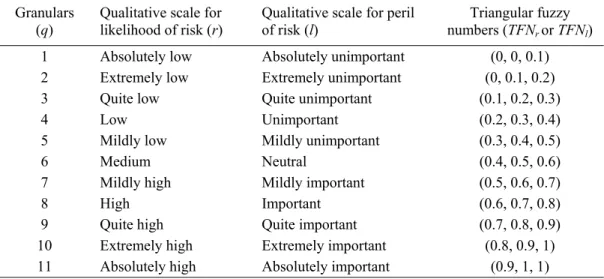
Let the likelihood r of failure be defined by the triangular fuzzy number TFNr and the consequence (or peril)

l of failure be defined by TFNl. Table 1 describes an 11-grade (or 11-granulars, q) qualitative scaling system

for both factors r and l (after Lee, 1996). The TFN definitions can be changed or modified based on expert opinion or on Delphi method-based surveys.

Table 1. Linguistic definitions of grades (granulars) using TFNs for likelihood and peril Granulars

(q)

Qualitative scale for likelihood of risk (r)

Qualitative scale for peril of risk (l)

Triangular fuzzy numbers (TFNr or TFNl) 1 Absolutely low Absolutely unimportant (0, 0, 0.1) 2 Extremely low Extremely unimportant (0, 0.1, 0.2) 3 Quite low Quite unimportant (0.1, 0.2, 0.3)

4 Low Unimportant (0.2, 0.3, 0.4)

5 Mildly low Mildly unimportant (0.3, 0.4, 0.5)

6 Medium Neutral (0.4, 0.5, 0.6)

7 Mildly high Mildly important (0.5, 0.6, 0.7)

8 High Important (0.6, 0.7, 0.8)

9 Quite high Quite important (0.7, 0.8, 0.9) 10 Extremely high Extremely important (0.8, 0.9, 1) 11 Absolutely high Absolutely important (0.9, 1, 1)

Failure risk is defined as the product of the fuzzy numbers denoting r and l (equivalent to defining risk as the joint probabilities of occurrence and consequences provided the representative probabilities are independent). By definition, the product of two TFNs is itself a TFN. Let TFNr be defined by the members (ar, br, cr) and

TFNl by (al, bl, cl). The risk TFNrl for these r and l is then calculated by

TFNrl = TFNr× TFNl = (ar * al, br * bl, cr * cl) (1)

TFNrl a fuzzy number can be ‘defuzzified’. Defuzzification is a process to determine a crisp or point estimate

of a fuzzy number. A defuzzified value is generally defined by the centroid using the moment of area method (Yager, 1980). Defuzzified risk = ( ) ( ) ( ) ( ) ∫ ∫ ⋅ = l c * r c l a * r a rl rl l c * r c l a * r a rl rl rl dx ) x ( dx ) x ( x ) l , r ( g µ µ (2)

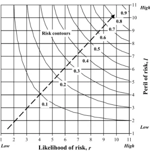
Figure 2 depicts the risk contours representing defuzzified risk g(r,l). The reason for this defuzzification is explained below.

1 2 3 4 5 6 7 8 9 10 11 1 2 3 4 5 6 7 8 9 10 11 Likelihood of risk, r Peril o f risk, l 0.1 0.2 0.3 0.4 0.5 0.6 0.7 0.8 0.9 Risk contours Low Low High High

Figure 2. Contours to estimate defuzzified risk g(r, l) for basic risk items

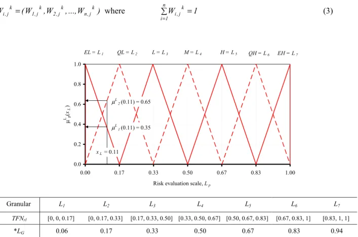
Let L1 through L7 denote seven-grades (or granulars, p) in a scale system for risk magnitude. In this system,

the qualitative variables are - extremely low (EL), quite low (QL), low (L), medium (M), high (H), quite high (QH) and extremely high (EH). Figure 3 shows a graphical representation of the risk grades with their membership functions (TFNs). This seven-grade system will be used to quantify risk in linguistic terms. Consequently, TFNrl has to be expressed in terms of L1 through L7. This cannot be done directly because

TFNrl is derived from two TFNs with 11 granulars each. Instead, the defuzzified value xL = g(r,l) is mapped

into the 7-grade risk scale using the appropriate membership functions. For the example given in Figure 3, the membership values of xL = 0.11 to L1 and L2 are 0.35 and to 0.65, respectively. The fuzzy number

representing xL is the 7-tuple fuzzy number X= {0.35, 0.65, 0, 0, 0, 0, 0}, in which each tuple represents the

membership value of xL to each of the seven grades in the system. This can also be expressed as

      = EH 0 , QH 0 , H 0 , M 0 , L 0 , QL 65 . 0 , EL 35 . 0

X , where the denominators are the names of the corresponding

grades.

3. The Structure of Hierarchical Model

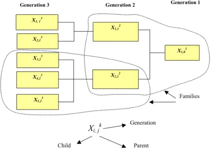
Figure 4 and Table 2 illustrate the basic building blocks of the hierarchical structural model. Essentially, each risk item is partitioned into its contributory factors, which are also risk items, and each of those can be further partitioned into lower level contributory factors. The unit consisting of a risk factor (“parent”) and its contributory factors (“children”) is called the “family”. A family consists of two generations but each of the children can be further partitioned into children of the next generation. A risk element with no children is called “basic risk item”, while the term risk item or risk attribute are interchangeably used for all elements with offspring.

The notation used for a risk item or attribute is Xi,jk, where i is the ordinal number of risk item X in the current

generation; j is the ordinal number of the parent (in the previous generation); and k is the generation order of X. In Table 2, the factors ri,jk and li,jk respectively denote likelihood and peril for the risk item Xi,jk. When the

respective contributions of sibling risk items towards their parent are non-commensurate in their units (e.g., one is quantified as financial loss, while the others are quantified in terms of environmental damage), a weighting scheme is required. Table 2 shows the general case where weights are assigned to each risk item. The notation used is Wi,jk, which denotes the weight of Xi,jk relative to its siblings. The weights are estimated

using analytic hierarchy process (AHP) and the details are given in the following paragraphs. When the respective contributions of sibling risk items towards their parent are commensurate in their units, then Wi,jk

are equal for all the siblings.

The analytic hierarchy process (AHP) is a technique commonly used for multiple-criteria analysis. The AHP develops a linear additive model, which derives weights by performing pair-wise comparisons between criteria or attributes (Ziara et al., 2002). Saaty (1988,1996) defined a 9-level scale for relative importance used in this process of pair-wise comparisons. These levels range from equal importance through strong importance up to extreme importance. Saaty (1988, 2001) describes complete details of the procedure to derive weights from the relative importance scale. These weights are normalized to a sum of 1, such that in any generation (k), for n siblings with parent j, a set of weights can be written as

) W ..., , W , W ( W_i,jk = _1,jk _2,jk _n,jk where ∑ = (3) = n 1 i k j , i 1 W 0.0 0.2 0.4 0.6 0.8 1.0 0.00 0.17 0.33 0.50 0.67 0.83 1.00

Risk evaluation scale, Lp

µ L p (x L ) EL = L1 QL = L2 L = L3 M = L4 H = L5 QH = L6 EH = L7 xL = 0.11 µL 1(0.11) = 0.35 µL 2(0.11) = 0.65 Granular L1 L2 L3 L4 L5 L6 L7 TFNrl [0, 0, 0.17] [0, 0.17, 0.33] [0.17, 0.33, 0.50] [0.33, 0.50, 0.67] [0.50, 0.67, 0.83] [0.67, 0.83, 1] [0.83, 1, 1] *LG 0.06 0.17 0.33 0.50 0.67 0.83 0.94

*LG is the x-co-ordinate of the centre of gravity of a granular and is expressed as a vector LG = {0.06, 0.17, 0.33, ... , 0.94}

Figure 3. Seven-grade fuzzy scale for representing risk

Table 2. A hierarchical model for aggregative risk analysis

Xi,j3 ri,jk li,jk *g (ri,jk, li,jk) Wi,j3 Xi,j2 Wi,j2 †Xi,j1 X1,13 r1,13 l1,13 g (r1,13, l1,13) W1,13 X1,12 W1,12 X1,01 X2,13 r2,13 l2,13 g (r2,13, l2,13) W2,13

X3,23 r3,23 l3,23 g (r3,23, l3,23) W3,23 X2,12 W2,12 X4,23 r4,23 l4,23 g (r4,23, l4,23) W4,23

X5,23 r5,23 l5,23 g (r5,23, l5,23) W5,23

Parent Child

Generation 3 Generation 2 Generation 1

X1, 13 X2,1 3 X3,23 X4,2 3 X5,2 3 X2,1 2 X1,01 X1,1 2 Families Xi, j k Generation

Figure 4. A hierarchical structure for the estimation of aggregative risk

Aggregation of fuzzy sets require operations by which several fuzzy numbers are combined in a desirable way to produce a single fuzzy number (Klir and Yuan, 1995). Although there are various ways to aggregate fuzzy sets, in this study, the weighted average technique was used to aggregate risk.

The process of evaluating aggregative risk in a fundamental unit (i.e., “family”) of the aggregative structure can now be summarized, using the family (Figure 4) of X2,12 (parent) and X3,23, X4,23, X5,23(children) as an

example. For each of the sibling risk items, the likelihood r and peril l are estimated using the 11-grade scaling system (Table 1). Their respective TFNr and TFNl values are then multiplied to obtain their TFNrl

values (equation 1), which are then defuzzified using equation (2) to obtain the respective values for g(r,l). These values are then mapped into the 7-grade risk scale (Figure 3), to obtain the 7-tuple fuzzy numbers X3,23, X4,23, X5,23representing the risk contribution of each of the siblings towards their parent. For ease of

manipulation these 7-tuple numbers can be arranged in a fuzzy assessment matrix (FAM), which is a 3 × 7 matrix F(Xi,23), where the index j = 2 stands for siblings of parent item number 2 in the previous generation.

The AHP is then applied and weights W3,23, W4,23, W5,23are evaluated and arranged into a 3-member vector.

The aggregative risk (or parent or risk attribute) of the three siblings is a 7-tuple fuzzy number X2,12which is

calculated by

[

]

[

]

where µpL (p = 1, 2,…, 7) are the membership values of the aggregated risk with respect to a 7-grade risk

scale. The aggregation of risk towards the next level (next generation) is done in the same way.

The process of evaluating r and l and re-mapping the product risk into the 7-grade risk scale, is done only for basic risk items (those risk items which do not have children). Consequently it is useful to use notation that distinguishes between basic and non-basic risk items. In the remainder of this paper, the notation for a basic risk item will include an apostrophe at the generation index, i.e., if item X4,23 is a basic risk item, it will be

denoted X4,23’. It should also be noted that in the first generation of the structure (i.e., the head of the

pyramid) the final aggregative risk can be defuzzified to provide a single (crisp) measure of the risk of the entire structure. This can be determined by

Defuzzified risk = L_G⋅X_1,01 (5)

where LG is the 7-member vector defined in Figure 3. The defuzzified risk is calculated as a dot product of

vector LG and fuzzy number X1,01.

4. An Application of the Proposed Methodology

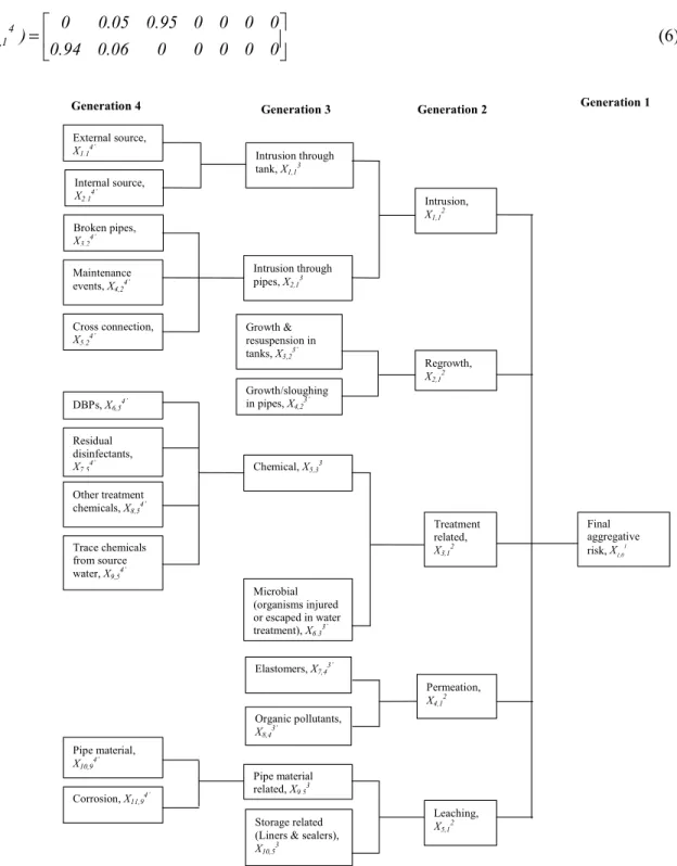
Figure 5 shows a simplified hierarchical structure for water quality failure. The detailed discussion on each type of water quality failure can be seen in Sadiq et al. (2003). This structure is used to demonstrate the aggregative risk framework introduced earlier. Table 3 lists the 17 basic risk items for the proposed structure. These basic risk items are grouped into third generation risk attributes, which in turn are grouped into second generation risk attributes including intrusion, regrowth, water treatment related, permeation and leaching. The weight matrices Wi,jk for each set of siblings were developed using an AHP technique as discussed

before.

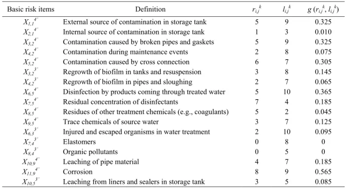
Table 3. Complete data set for basic risk items for the evaluation of final aggregative risk Basic risk items Definition ri,jk li,jk g (ri,jk, li,jk)

X1,14’ External source of contamination in storage tank 5 9 0.325 X2,14’ Internal source of contamination in storage tank 1 3 0.010 X3,24’ Contamination caused by broken pipes and gaskets 5 9 0.325 X4,24’ Contamination during maintenance events 2 8 0.075 X5,24’ Contamination caused by cross connection 6 7 0.305 X3,23’ Regrowth of biofilm in tanks and resuspension 3 8 0.145 X4,23’ Regrowth of biofilm in pipes and sloughing 2 7 0.065 X6,54’ Disinfection by products coming through treated water 5 10 0.365 X7,54’ Residual concentration of disinfectants 7 4 0.185 X8,54’ Residues of other treatment chemicals (e.g., coagulants) 5 2 0.045

X9,54’ Trace chemicals of source water 3 7 0.125

X6,33’ Injured and escaped organisms in water treatment 2 10 0.095

X7,43’ Elastomers 0 8 0

X8,43’ Organic pollutants 0 5 0

X10,94’ Leaching of pipe material 4 7 0.185

X11,94’ Corrosion 8 9 0.565

X10,53’ Leaching from liners and sealers in storage tank 3 5 0.085

4.1. First stage risk aggregation

The first stage aggregation process is applied to only basic risk items. For each basic risk item r and l are assigned and then defuzzified to obtain the risk scalar g(ri,jk, li,jk). It should be noted that a basic risk item can

be in any generation in the hierarchical structure. The g(ri,jk, li,jk) values are then mapped on the 7-grade risk

scale to estimate their membership µpL(x) to the seven risk levels L1 to L7. For example, for basic risk item

7-grade risk scale are L1 = 0, L2 = 0.05, and L3 = 0.95 and L4 to L7 = 0 . The same procedure is applied to X2,14’

and subsequently, F(Xi,14) matrix can be formed as

      = 0 0 0 0 0 06 . 0 94 . 0 0 0 0 0 95 . 0 05 . 0 0 ) X ( F _i,14 (6)

Generation 4 _{Generation 3 Generation 2} Generation 1

External source, X1,14’ Internal source, X2,1 4’ Broken pipes, X3,24’ Maintenance events, X4,24’ Cross connection, X5,24’ Growth & resuspension in tanks, X3,23’ Intrusion through pipes, X2,13 Growth/sloughing in pipes, X4,23’ DBPs, X6,54’ Residual disinfectants, X7,54’ Chemical, X5,33 Other treatment chemicals, X8,54’ Trace chemicals from source water, X9,5 4’ Microbial (organisms injured or escaped in water treatment), X6,33’ Final aggregative risk, X_1,01 Intrusion, X1,12 Treatment related, X3,12 Elastomers, X7,43’ Organic pollutants, X8,43’ Regrowth, X2,12 Permeation, X4,1 2 Pipe material, X10,9 4’ Corrosion, X11,94’ Intrusion through tank, X1,13 Pipe material related, X9,53 Storage related (Liners & sealers), X10,5

3

Leaching, X5,1

2

Figure 5. Hierarchical structure for aggregative risk of water quality failure

This process is applied to all the families containing basic risk items and the fuzzy risk assessment matrices are established. These fuzzy risk assessment matrices are then multiplied by their respective weights. For example, F(Xi,14) is multiplied by weights W1,14 and W2,14 to determine the risk item X1,13

[

] [

]

[

X_1,13 = _1,14 _2,14 × _i,14 =

]

Similarly, all the other first stage aggregative risk items can be determined. The risk items estimated in the first stage aggregation can now be used to evaluate the aggregative risk items in the next stage.

4.2. Intermediate stage(s) risk aggregation

The intermediate stage risk aggregation is applied to all non-basic risk items except those feeding into the head of the pyramid. In the intermediate stage, the risk items from the previous stage are weighted and grouped to obtain the aggregated risk in the next generation. For example, X1,13 and X2,13 are multiplied by

W1,13 (= 0.33) and W2,13 (= 0.67) to obtain the intermediate risk item X1,12

[

]

[

]

All other intermediate risk items are determined following the same steps. These risk items can now be used to evaluate the aggregative risk items in the final stage.

4.3. Final stage risk aggregation

To obtain the final risk item X1,01 (head of the pyramid), the intermediate stage aggregative risk items X1,12,

X2,12, X3,12, X4,12 and X5,12 are arranged to form the fuzzy risk assessment matrix F(Xi,12), which is then

multiplied by the corresponding weights W1,12 (= 0.39), W2,12 (= 0.21), W3,12 (= 0.20), W4,12 (= 0.07) and W5,12

(= 0.13)

[

]

[

]

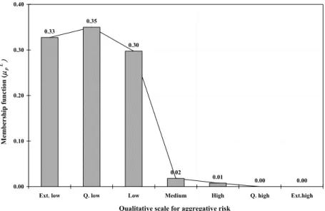
X1,01 is the final aggregative risk item. It is a 7-tuple fuzzy number, which can be expressed as

      = EH 0 , QH 0 , H 01 . 0 , M 02 . 0 , L 30 . 0 , QL 35 . 0 , EL 33 . 0 X_1,01 (11)

Equation (11), also called a possibility mass function, is plotted in Figure 6. The final defuzzified aggregative risk is determined by the multiplication of the centroids of membership functions LG and the 7-tuple fuzzy

number X1,01 as in equation (5). In this example, the final defuzzified risk value is L X 0.19. 1

0 , 1

0.33 0.35 0.30 0.02 0.01 0.00 0.00 0.00 0.10 0.20 0.30 0.40

Ext. low Q. low Low Medium High Q. high Ext.high

Qualitative scale for aggregative risk

Membership function (

µp L)

Figure 6. Possibility mass function for final aggregative risk of water quality failure

5. Summary and Conclusions

The structure presented in this paper is a simplified demonstration of the approach. A comprehensive structure would require a major effort, including the collaboration of several experts in various disciplines of knowledge. The proposed hierarchical aggregative risk approach has several advantages:

• It enables the synthesis of both quantitative and qualitative information into a single framework; • It can explicitly consider and propagate uncertainties;

• It is scalable and possesses a modular form; therefore, the addition of new knowledge and information can be accommodated at any stage and in any form, e.g., vulnerability to terrorist acts (safety related risk), hydraulic failure, financial risk etc. can be part of this framework;

• It can be used for cost-benefit analysis to facilitate efficient budget allocation and prioritize attention to those areas which have the most adverse impact on total system risk

• More data results in lesser uncertainty, which, when propagated through the hierarchical structure, can result in reduced total risk. The proposed approach can help pinpoint those areas in which more data would yield the highest benefits.

• It is easily programmable for computer applications and can become a risk analysis tool for a water distribution system.

The limitations of the proposed method are:

• It may be sensitive to the selection of aggregation operators. Different operators can be used for different segments of the model and trial and error approach can be used to avoid exaggeration (it occurs when all basic risk items are of relatively low risk, yet the final aggregative risk comes out unacceptably high), and

eclipsing (it occurs when one or more of the basic risk items is of relatively high risk, yet the estimated aggregative risk comes out as unacceptably low); and

• This framework supports both qualitative and quantitative data. Some data may be supported by rigorous observations, while other data may be based on loosely supported or anecdotal-based beliefs. These two types of data should have different weights in the aggregation process. The hierarchical structure in its current form does not address this need to distinguish between data obtained from sources of different reliabilities.

In the model development stages, the final aggregative risk value is expected to have limited meaning for the acceptability level of the risk to the general public. It is envisaged that as this hierarchical structure is

developed, populated and subsequently improved upon (using newly obtained data) the developers will gain insight into acceptable risk levels as they are manifested in the final fuzzy and/or defuzzified risk values. In the longer term, this approach could serve as a basis for bench marking acceptable risks in water distribution systems.

6. References

Kleiner, Y. 1998. Risk factors in water distribution systems, British Columbia Water and Waste Association 26th Annual Conference, Whistler, B.C., Canada.

Klir, G.J., and Yuan, B. 1995. Fuzzy sets and fuzzy logic - theory and applications, Prentice- Hall, Inc., Englewood Cliffs, NJ, USA.

Lee, H.-M. 1996. Applying fuzzy set theory to evaluate the rate of aggregative risk in software development, Fuzzy Sets and Systems, 79: 323-336.

Ricci, P.F., Sagen, L.A., and Whipple, C.G. 1981. Technological risk assessment series E: Applied Series No.81.

Saaty, T.L. 1988. Multicriteria decision-making: the analytic hierarchy process, University of Pittsburgh, Pittsburgh, Pa, USA.

Saaty, T.L. 1996. Decision making with dependence and feedback: the analytic hierarchy process, RWS, Pittsburgh, Pa, USA.

Saaty, T.L. 2001. How to make a decision? Chapter 1, Models, methods, concepts and applications of the analytic hierarchy process, Ed. Saaty, T.L., and Vargas, L.G., Kluwer International Series.

Sadiq, R., Kleiner, Y., and Rajani, B. 2003. Aggregative risk analysis for water quality in distribution networks, Submitted to Water Resources Research.

Yager, R.R. 1980. A general class of fuzzy connectives, Fuzzy Sets and Systems, 4: 235-242.

Zadeh, L.A. 1996. Fuzzy logic computing with words, IEEE Transactions – Fuzzy Systems, 4(2): 103-111. Ziara, M., Nigim, K., Enshassi, A., and Ayyub, B.M. 2002. Strategic implementation of infrastructure