Characterization of solar X-ray response data from the REXIS instrument

(1)

Characterization of Solar X-ray Response Data from the REXIS Instrument by

Andrew T. Cummings

S.B., Physics and S.B., Earth, Atmospheric, and Planetary Sciences Massachusetts Institute of Technology, 2020

Submitted to the MIT Department of Earth, Atmospheric, and Planetary Sciences and Department of Aeronautics and Astronautics in Partial Fulfillment of the Requirements for the Degrees

of

Master of Science in Earth, Atmospheric, and Planetary Sciences and Master of Science in Aeronautics and Astronautics

at the

Massachusetts Institute of Technology September 2020

Author . . . Department of Earth, Atmospheric, and Planetary Sciences Department of Aeronautics and Astronautics August 18, 2020 Certified by. . . . . . Richard P. Binzel Professor of Planetary Sciences Thesis Supervisor Certified by. . . . . . Rebecca A. Masterson Principal Research Scientist Thesis Supervisor Certified by. . . . . . Branden T. Allen Research Scientist, Harvard College Observatory Thesis Supervisor Accepted by . . . . . .

Robert D. van der Hilst Schlumberger Professor of Earth and Planetary Sciences

Department Head Accepted by . . . . . .

Zoltan S. Spakovszky Associate Professor of Aeronautics and Astronautics Chair, Graduate Program Committee

(2)

(3)

Characterization of Solar X-ray Response Data from the

REXIS Instrument

by

Andrew T. Cummings

Submitted to the Department of Earth, Atmospheric, and Planetary Sciences and Department of Aeronautics and Astronautics

on August 18, 2020, in partial fulfillment of the requirements for the degree of

Master of Science in Earth, Atmospheric, and Planetary Sciences and Master of Science in Aeronautics and Astronautics

Abstract

The REgolith X-ray Imaging Spectrometer (REXIS) is a student-built instrument that was flown on NASA’s Origins, Spectral Interpretation, Resource Identification, Safety, Regolith Explorer (OSIRIS-REx) mission. During the primary science ob-servation phase, the REXIS Solar X-ray Monitor (SXM) experienced a lower than anticipated solar x-ray count rate. Solar x-ray count decreased most prominently in the low energy region of instrument detection, and made calibrating the REXIS main spectrometer difficult. This thesis documents a root cause investigation into the cause of the low x-ray count anomaly in the SXM. Vulnerable electronic components are identified, and recommendations for hardware improvements are made to better facilitate future low-cost, high-risk instrumentation. A CAST Analysis is conducted and programmatic recommendations for future student instruments are provided.

Thesis Supervisor: Richard P. Binzel Title: Professor of Planetary Sciences

Thesis Supervisor: Rebecca A. Masterson Title: Principal Research Scientist

Thesis Supervisor: Branden T. Allen

(4)

(5)

Acknowledgments

I conducted my work as a research assistant with the REXIS program in the Space Systems Laboratory as a student in the MIT Department of Earth, Atmospheric, and Planetary Sciences and the MIT Department of Aeronautics and Astronautics. I owe this thesis to the dedication of countless friends, loved ones, faculty, and staff. Though there are too many to list, I wish to acknowledge a few:

First and foremost, I would like to express my gratitude to Dr. Rebecca Mas-terson for her guidance and encouragement in the past year. Thank you for always challenging me to grow and improve as an engineer, and for always believing in me.

I would like to thank my other advisor, Professor Richard Binzel, who first invited me to join the REXIS project, and whose passion for science motivated me to dream big and start down this road. Thank you for recognizing something in me, and for agreeing to advise just one last time.

I could not have completed this thesis without the the help and guidance of Dr. Branden Allen. Thank you for always responding to my 2:00 AM emails and for pushing me to always ask the why questions. I hope that we can both get some sleep now that this thesis is complete. We need it.

AdditionallyI would like to recognize the Harvard-Smithsonian Center for Astro-physics team of Dr. Daniel Hoak, Dr. Jaesub Hong, and Professor Jonathan Grindlay for mentoring me. Many thanks to the REXIS cohort of Maddy Lambert, Carolyn Thayer, and David Guevel; I would do it all again for the laughs and camaraderie. Special thanks to Megan Jordan for tolerating endless paperwork and logistics, and at times, wrangling me in.

I would also like to thank my family for sending their love and support from so very far away. And to my friends: Lucy, Dan, Brandon, Ruth, Brendan, and Lara; Thank you for being the people who lifted me up when I was down, and for being with me all the way.

Lastly, I wish to thank the Halperin family and Lopez Island, Washington, for welcoming me into their home and community during an unprecedented global crisis.

(6)

(7)

List of Figures

1-1 A CAD model of the REXIS Main Spectrometer [8]. . . 21

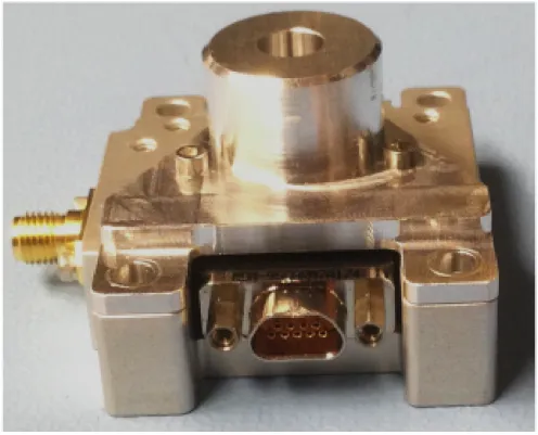
1-2 The REXIS Solar X-ray Monitor. . . 22

2-1 Common circuit elements. . . 28

2-2 A generic op-amp. (1) Inverting input, (2) Non-inverting input, (3) Positive power supply, (4) Negative power supply, (5) Output. . . 31

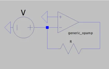
2-3 A generic op-amp with open-loop gain. . . 32

2-4 A generic op-amp with closed-loop gain. . . 33

2-5 An example differentiator circuit. . . 34

2-6 An example integrator circuit. . . 35

2-7 An integrator circuit with an additional resistor added to the feedback loop provides a discharge path for the capacitor. . . 35

2-8 An example Schmitt Trigger. . . 36

2-9 A spectral abundance model is created using the Chianti database. A simulated SXM response histogram shows instrument response based on the abundance model. Level 0 flight data from the SXM is matched to the simulated response histogram to generate single temperature fits and produce a time-dependent solar temperature plot. . . 39

2-10 An example safety control structure [13]. . . 42

3-1 The REXIS Requirements documentation flow from Jones, 2015 [7]. 45 3-2 SXM detector and preamp housing. The SXM detector is located below the collimator. . . 48

(12)

3-4 Schematic of SXM Amplification Chain. Outputs outb and outu are seen on the far right. The Outb opamp is configured as a differentiator circuit, and the outb opamp is configured as an integrator circuit. The three opamps behind the outu and outb opamps amplify the signal from the preamp. . . 49

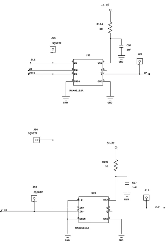
3-5 SXM Trigger Circuit Schematic. When outb exceeds VLLD, LLD

switches from 0 V to its on state at 2.4V. LLD’s rising action arms the ADC for detection. In the top comparator, when VB exceeds outb, ZP switches from its on setting to 0 V. ZP’s change of state tells the ADC to trigger, and coincides with the maximum of 𝑜𝑢𝑡𝑢1. . . 51

3-6 SXM signals at various points throughout the amplification chain [7]. outu is the output signal from the integrator circuit, and 𝑜𝑢𝑡𝑢1 is outu

minus an offset voltage. Outb is the output of the differentiator circuit. When outb exceeds VLLD, LLD goes high, arming the ADC. As outb falls below VLLD, LLD returns to 0 V. The zero point of outb where it crosses its steady state voltage coincides with the peak of 𝑜𝑢𝑡𝑢1. When

𝑜𝑢𝑡𝑢1 is at its maximum, ZP switches states and triggers the ADC. The

peak height of 𝑜𝑢𝑡𝑢1 is captured by the ADC and provides the energy

of the x-ray being detected. . . 52

3-7 A calibration histogram showing SXM response to an Fe-55 source. . 55

3-8 Set temperatures on the DE during Instrument Level TVAC Test, 2015. The DE is considered a proxy for MEB temperature because the DE records all boards housed in the REXIS Electronics Box where the MEB resides. The DE records lower temperature noise than the MEB, making the DE temperature sensor a more accurate measurement. . . 56

3-9 Instrument level testing results demonstrate a susceptibility in the MEB. The temperature recorded in this figure is of the MEB base plate and shows how temerature was cycled during the test. . . 56

(13)

3-10 Results of SXM Oven Test, November 2015. In this test, the preamp and detector were placed in the chamber, and the MEB was left out-side. This eliminated the possibility that the preamp was the source of thermal senstivity in SXM circuitry. The red curve is the temperature of the chamber, and the blue are x-ray data from the instrument. . . 57

3-11 Timeline of REXIS Operations highlighting instances where the SXM Low Count Rate anomaly was observed. . . 58

3-12 SXM Event Rate Histogram from L+6. The gain change is seen in the low and high energy artifacts, and suppresses signal as seen in the boxed region. . . 59

3-13 An event rate histogram from Pre-EGA. Subtle threshold changes are seen at 2 keV between 20,000 seconds and 35,000 seconds where the low energy zero point line disappears. High energy artifact shows a small gain change as well that is highlighted with red arrows at the top of the figure. The threshold must be high to suppress signal at 3keV. The reset artifact is eliminated as shown by the right red arrows. The elimination of the reset artifact indicates a gain change. The SXM is not pointing towards the sun between 45,000 and 70,000 seconds. . . 60

3-14 An event rate histogram from Post-EGA. A more drastic threshold change is shown to suppress the low energy at 2 keV. High energy artifacts disappear at the same time as signal is lost at 150 ADU, indicating that the threshold has gone high. The disappearance of high energy artifacts, shown with arrows, indicates a gain change. . . 61

3-15 SXM Event Rate Histograms at L+30. . . 62

3-16 SXM Event Rate Histogram from Orbital B, 25 July 2019. Low en-ergy x-ray signal sits at 2 keV, and counts are on the same order of magnitude as the low energy noise artifacts. The area with no data is when the SXM was not on. . . 64

(14)

3-17 SXM Event Rate Histogram from Orbital R, 13 November 2019. The SXM recorded a similar slow rate of low energy signal, which is shown at 2 keV. The gap in data occurred when the instrument was powered

off. . . 65

4-1 SXM count rate histogram from launch to Orbital R. Data are shown chronologically from left to right, and Orbital B data are shown in the center of the figure. Low energy x-ray data are shown at 100 ADU on the y-axis; there is a distinct dropoff in low energy signal during Orbital B and the first half of Orbital R, and then a more drastic decrease in signal during the second half of Orbital R. Orbital R data from the second half of the observation window have a low energy count rate similar to in-flight calibrations where the sun was not in the SXM’s field of view (FOV). . . 69

4-2 SXM Saturated Histogram (Right) and Corrected Histogram (Left) . 70 4-3 SXM count rate histogram on 18 November, 2019. The gap in the his-togram is when the instrument was not recording data, and is unrelated to the low count rate anomaly in Orbital R. . . 71

4-4 Fishbone diagram constructed for OSIRIS-REx ISA #10939 . . . 72

4-5 Flare Coincidence between the SXM and GOES15. . . 74

4-6 SXM longterm HV for its operational lifetime. . . 75

4-7 The longterm temperature of the SXM. The increase in MEB temper-ature can be seen in Orbital R and Orbital B. Orbital R is hotter than Orbital B and the MEB saw temperatures similar to EGA. . . 77

(15)

4-9 SXM Histogram comparison of before and after low count rate anomaly. Low energy is lost in the 80-150 ADU range in Orbital B and Orbital R data. High Energy matches previous data taken in internal calibra-tion. Artifacts seen at 90 ADU, 0 ADU, and 512 ADU remain constant throughout observation, indicating that there was no gain change dur-ing Orbital B and Orbital R. . . 79

4-10 A block diagram of the resistance coupling configuration used in SXM threshold simulations. The resistive couplings are boxed in blue. The resistors in the feedback loops for the opamps are more complex than what is shown in the figure and feedback loops contain both capacitors and resistors to shape the feedback signal. . . 82

4-11 The VLLD voltage switching thresholds for different magnitudes of resistance coupling. When VLLD exceeds the top threshold value, outb settles to a low quiescent value. Likewise, when VLLD is lower than the low switching threshold, outb shifts to its high quiescent value. 83

4-12 Time-dependent resistance coupling for outu and outb demonstrating the hysteresis effect in resistive coupling. The coupling resistance was increased over time in order to identify potential coupling strengths of interest that matched the flight phenomenon. The area between 1000Ω and 10,000Ω is a region of interest in we see a little variation in the gain (outu), and a large variation in the threshold (outb). . . 84

4-13 Results of constant threshold test. This case depicts a 2 keV x-rfay signal passing through the SXM amplification chain and triggering. VLLD does not vary in this experiment. . . 85

4-14 Results of Set-High-Set threshold test. This Case most resembles the startup sequence used for the SXM during flight. Outb settles after VLLD returns to its starting value. At 5𝜇s, the preamp signal pulses, after which outu andoutb show a characteristic response. The voltage response from outb rises above VLLD and triggers a detection. . . 86

(16)

4-15 Results of Set-Low-Set threshold test. Outb settles after VLLD returns to its starting value. At 5𝜇s, the preamp signal pulses, after which outu andoutb show a characteristic response. However, the voltage response from outb is suppressed and does not rise above VLLD and does not trigger a detection. . . 87

5-1 High level safety control structure. The red box outlines the CAST boundary for this analysis. . . 96 5-2 The SXM safety control structure being studied in this chapter . . . . 96

C-1 Email correspondence outlining changes made to the SXM during Fall 2015. . . 139

(17)

List of Tables

3.1 Quantum Efficiency Requirements for the SXM Detector. . . 46

3.2 SXM Level 3 Requirements [7]. . . 47

3.3 SXM Level 4 Requirements [7]. . . 47

(18)

List of Acronyms

ADC Analog-to-Digital Converter

CAST Causal Analysis based on System

Theory

CXB Cosmic X-ray Background

DE Detector Electronics

EAPS Earth, Atmospheric, and

Plane-tary Sciences

EBOX Electronics Box

FOV Field of View

HCO Harvard College Observatory

LLD Lower Limit Discriminator

MBU Multi-Bit Upset

MEB Main Electronics Board

MKI MIT Kavli Institute for

Astro-physics and Space Research

Opamp Operational Amplifier

OSIRIS-REX Origins, Spectral Interpretation,

Resource Identification, Security, Regolith Explorer

PCB Printed Circuit Board

PI Principle Investigator

PM Project Manager

REXIS Regolith X-ray Imaging

Spec-trometer

SDD Silicon Drift Diode

SEU Single Event Upset

SSL Space Systems Laboratory

SXM Solar X-ray Monitor

VLLD Voltage Lower Limit

(19)

Chapter 1 Introduction

This thesis provides an overview of operations involving the REXIS Solar X-ray Mon-itor (SXM), and a root cause investigation into the cause of unanticipated low solar signal seen during data collection. The SXM is a complementary instrument to the REgolith X-ray Imaging Spectrometer (REXIS), which is mounted aboard NASA’s OSIRIS-REx mission.

The REXIS instrument was designed to produce elemental abundance maps of the surface of the asteroid 101955 Bennu, a C-type near-Earth asteroid using spectrom-etry. Bennu is of particular interest because it has a 1-in-2700 chance of impacting Earth between 2175 and 2199 [12].

REXIS is a low-cost, high-risk payload. Isolating the root cause of the malfunc-tion and identifying critical components that resulted in failure will provide future projects with additional knowledge for instrument design. The SXM detects variable x-ray flux from the Sun, which is used to measure solar temperature and spectral abundance. This thesis provides an explanation of how solar x-rays are captured by the SXM and how signal data are interpreted. Solar spectra analysis and solar temperature fitting techniques are discussed, as well as the limitations of SXM model-ing. SXM amplification electronics hardware and signal processing is discussed, with a focus on the analog signal amplification chain and threshold trigger circuit. An operational timeline of the SXM is presented and observation results are discussed. The focus of the latter portion of the thesis is a root cause analysis of the low x-ray

(20)

count-rate anomaly that occurred late in the SXM’s operational lifetime. This thesis concludes with a roadmap for future work, including a more complete root cause in-vestigation into thermal sensitivity, and a CAST analysis to highlight organizational and programmatic controls that may have contributed to the drop off in x-ray counts.

1.1 REXIS Mission

REXIS is a student experiment developed initially as part of the 2011 undergraduate capstone class in the Department of Aeronautics and Astronautics at MIT. Construc-tion and management of the instrument was conducted in the MIT Space Systems Laboratory (SSL) as part of a larger collaboration with Harvard College Observatory (HCO), the MIT Department of Earth, Atmospheric, and Planetary Science, the MIT Kavli Institute (MKI), MIT Lincoln Laboratories, and Aurora Flight Sciences. Day-to-day operations and engineering are conducted primarily by students with guidance from senior faculty and staff including Professor Richard Binzel, the REXIS Instru-ment Scientist, Professor Jonathan Grindlay, the REXIS Deputy InstruInstru-ment scientist from HCO, and Dr. Rebecca Masterson, the REXIS Project Manager, from the MIT Department of Aeronautics and Astronautics. To date, over 80 students have worked on REXIS at all levels and stages of the project.

The REXIS main spectrometer uses x-ray spectroscopy to capture incident x-rays from Bennu’s surface in the soft x-ray band (0.5-7.5 keV). A total x-ray spectrum is derived from the soft x-ray data and REXIS was designed to detect, if measurable, signals from Si, S, Mg, and O. In imaging mode, REXIS maps specific abundances to locations on Bennu’s surface with necessary spatial resolution at an observation distance of 700m. In spectral mode, REXIS records x-ray energies and produces the global average of the x-ray spectrum passing through the coded aperture mask [20]. REXIS performs its science objective independent of the other OSIRIS-REx instruments [11],[15].

A CAD model of REXIS is shown in Figure 1-1. The primary components of REXIS are housed in the main instrument. The main spectrometer detector consists

(21)

of a 2x2 array of CCD’s housed within a coded aperture mask. Housed separately is the Solar X-Ray Monitor (SXM), that captures solar x-ray data with a single SDD detector (Figure 1-2.) The SXM is the focus of this study. The SXM is an x-ray

Figure 1-1: A CAD model of the REXIS Main Spectrometer [8].

detector attached externally to the spacecraft bus, near the high gain antenna, so that it would be sun facing during observations of Bennu. The SXM detector is mounted to the outside of the spacecraft, and detector electronics are connected via a coax to the Main Electronics Board (MEB), located inside the spacecraft.

REXIS is the second student experiment to accompany a New Frontiers mission as part of NASA’s education and public outreach initiative. The first student instru-ment, the Venetia Burney Student Dust Counter (VBSDC, formerly SDC) built by University of Colorado Boulder, flew on the New Horizons spacecraft and recorded interplanetary dust from between 2.6 and 15.5 AU [19]. REXIS is a significant leap in complexity from the VBSDC, and is meant to directly involve students with all parts of spacecraft instrumentation development and operations.

(22)

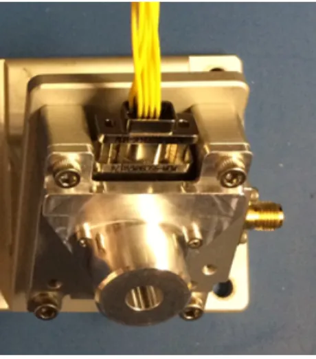
Figure 1-2: The REXIS Solar X-ray Monitor.

1.2 REXIS Operational Timeline

This section discusses the operational lifetime of REXIS and the SXM, from its launch on 8 September 2016 until the conclusion of the instrument’s science mission follow-ing the OSIRIS-REx Orbital R mission phase in November 2019. A more detailed explanation of SXM operations can be found in Chapter 3. Henceforth, some opera-tional times will be referred to as "L+", which stands for months after launch, unless otherwise specified. For example, events in the L+30 phase of the mission occurred 30 months after launch.

REXIS was powered on during L+14 Days for a payload inspection and functions check. The SXM took 3935 seconds of x-ray data, and the instrument function was nominal. The SXM was turned on for an additional function check at L+6, where the instrument threshold was set. A third functions check was conducted during L+18. The SXM remained nominal, and there were no anomalies in x-ray detection.

(23)

the SXM were again checked for behavioral anomalies. Data collected by the SXM demonstrated that the SXM was able to collect solar x-ray data. During L+22, REXIS was internally calibrated to identify background noise and hot pixels. As a diode detector, the SXM cannot have hot pixels in the same way as a charge-coupled device (CCD) detector. The SXM was not facing the sun during L+22 and recorded nominal cosmic x-ray background (CXB).

REXIS performed its cover opening operation in September 2018. The radiation cover was released using a frangibolt, after which REXIS detectors were first exposed to the space environment. REXIS underwent a series of cosmic x-ray calibrations (CXB), and the REXIS spectrometer was shown to be sensitive to stray light.

The L+30 Calibration was the first time Bennu was observable in the REXIS field of view. During this calibration, a hot pixel mask was tested on REXIS. SXM count rates were lower than previous observations, but returned to previously seen levels in later flight.

During flight, REXIS underwent a series of calibrations using the Crab Nebula and Scorpius X-1 (Sco-X-1), two known cosmic ray sources. Using a known, stable x-ray emitter provided a source that allowed the gain and offset of the REXIS detector nodes to be set. Crab Calibration took place in November 2018 and March 2019, while Sco X-1 occurred later, during Mask Calibration.

Orbital B, the first REXIS observation phase, occurred from 1 July to 6 August, 2019. Orbital B was initially the only planned observation window for the REXIS instrument. The OSIRIS-REx spacecraft was placed in a stable orbit one kilometer above the surface of Bennu. The SXM count rate saturation anomaly was found during Orbital B, where the instrument reported abnormally high counts on the detector. On 5 July, SXM data was saturated with an additional value of 34880. It was believed that a multi-bit upset (MBU) occurred, where radiation moved the reset value on the SXM. The multi-bit upset (MBU) error was corrected with a reset

command from the ground. Additionally, throughout Orbital B the SXM began

showing a two order of magnitude decrease in x-ray signal that was unexplained by the spacecraft’s increase in solar distance. The results from results from the SXM’s

(24)

Internal Calibration are depicted in Figure 4-1. More on this anomaly can be found in Chapter 4. In all, two anomalies were detected in the SXM, and three were detected in the main spectrometer. For more information on REXIS anomalies, consult Maddy Lambert’s thesis [9].

Orbital R was the final observation window for REXIS, which occurred during November 2019. The REXIS team petitioned for, and was awarded, this additional observation to supplement limited data taken during Orbital B.

1.3 Motivation

The REXIS project was developed with the philosophy of being a low cost, high risk student instrument. From its inception as the final deliverable for 16.83, the MIT Aerospace Engineering senior design capstone class, undergraduate and gradu-ate students worked side-by-side with experienced research scientists and engineers. Students directly applied skills learned in their undergraduate curricula, and pro-duced an instrument of complexity, scale, and mission worthy of being included on a New Frontiers spacecraft. Like all projects, there were challenges faced along the way. A rotating ensemble of students created a challenging environment for informational and experiential entropy.

The REXIS instrument is contracted as a "Do No Harm" mission, which is char-acterized by lower cost and the use of legacy hardware [17]. Indeed, a portion of the electronics design process for REXIS consisted of utilizing existing schematics from NICER, an x-ray instrument developed by the MIT Kavli Institute (MKI). These schematics were simplified for the design of the SXM as a matter of reducing cost. Identifying the source of the SXM spaceflight anomaly not only provides guidance on potential hardware vulnerabilities which exist in current spaceflight missions; it also yields a roadmap for future missions. Often, mission rely on heritage hardware com-ponents to cut down on integration and testing time, but this can be deceptive. As this thesis discusses later on, relying on heritage hardware without proper considera-tion for an instrument’s unique mission creates a hazardous development environment

(25)

where an instrument is not properly tested.

The SXM experienced lower than anticipated x-ray counts during the Orbital B and Orbital R phases of flight. SXM data during this time were unable to be fit to solar temperature models, and the integrity of SXM function was called into question. The lack of low energy x-ray events during Orbital B launched a root cause investigation to trace the cause of low signal. The MEB inherited signal amplification design heritage with the NICER instrument, which is an ongoing project. Isolating the root cause of low x-ray signal benefits future x-ray instrumentation instruments and existing instruments that use similar signal shaping electronics. This thesis presents a CAST analysis of the root cause of the low x-ray count rate anomaly, and provides recommendations for future low cost, high risk instrumentation.

1.4 Thesis Roadmap

This thesis is organized into six chapters that document the SXM background, in-strument anomaly, root cause investigation, and CAST analysis. Chapter 2 presents a background on the SXM, including an explanation of the SXM data pipeline and associated solar x-ray modeling. A broad overview of the electronic components that comprise the SXM is provided, as well as how they operate in the space environment. In Chapter 3, the structure and design process of the SXM is explained in greater detail. Chapter 3 continues with a summary of instrument development testing that occurred, both on the ground and after launch. Then, SXM flight operations leading up to and after the anomaly are discussed. Chapter 4 explores the SXM low x-ray count rate anomaly and root cause analysis. The identification of the low count-rate anomaly is explained in depth. Chapter 4 ends with a plan for future research into the identification of the vulnerability that caused the anomaly and how such a find-ing may be interpreted. Chapter 5 summarizes a CAST analysis conducted around the findings of the root cause investigation and provides recommendations for fu-ture instruments with similar project scope. Chapter 6 concludes with a summary of the low x-ray count rate root cause investigation and CAST analysis, and provides

(26)

(27)

Chapter 2 Background

This chapter describes the circuitry used in the SXM. The SXM relies on an intricate array of amplifiers and filters, which are capable of x-ray detection when combined. The chapter begins with an introduction of standard electrical components and how they operate. An example circuit of each component is provided and includes a visual representation of ideal operation. Chapter 2 creates a foundation of understanding that creates a background to discuss the more complex electrical engineering systems seen in the SXM. The first advanced concept explained is signal amplification. Sig-nal amplification is the primary means through which a sigSig-nal is passed from the SXM detector and recorded by the instrument. Typical amplification techniques are compared against amplification used in the SXM. To understand signal processing in the SXM, an explanation of analog-to-digital conversion is provided. A more thor-ough model of SXM signal processing is covered later in the chapter. The thermal sensitivity of electrical systems is explained, and typical response sensitivities are modeled. An overview of the SXM explains the functions of the instrument and how an x-ray signal is processed. A theoretical solar x-ray response is traced from initial detection, through the pipeline, and finally to transmission to the ground. The SXM Data Pipeline is explained from end-to-end. Finally, the chapter concludes with the modeling of theoretical instrument response using the Chianti Atomic Database and an explanation of how it is implemented in the Data Pipeline. Appendix A contains electrical schematics for the SXM amplification chain and trigger circuit. SXM solar

(28)

A

B

C

Figure 2-1: Common circuit elements.

temperature modeling simulation code can be found in Appendix B. Appendix C contains select emails used to gather information for the CAST analysis. Appendix D contains LTSpice code used to replicate the SXM amplification circuit and trigger.

2.1 Basic Circuitry

This section introduces the common electrical components used in the SXM, how they operate individually, and how they are used together to create more complex circuitry.

2.1.1 Common Components

Resistor

A resistor is an electrical element with a positive and negative terminal that utilizes the property of electrical resistance. Its primary functions include voltage division, current flow reduction, and signal reduction. Ideal resistors function based on Ohm’s law,

(29)

where the voltage differential across the resistor is proportional to the product of current and resistivity. Resistors are commonly used in two constructions: parallel and series. Resistors in parallel are be treated as the multiplicative inverse of the sum of the reciprocals of individual resistors,

1 𝑅𝑒𝑞 = 1 𝑅1 + 1 𝑅2 + · · · + 1 𝑅𝑛 . (2.2)

Series resistors are treated as the sum of individual resistances,

𝑅𝑒𝑞 = 𝑅1+ 𝑅2+ · · · + 𝑅𝑛. (2.3)

.

In practical application, resistors are susceptible to series induction and parallel capacitance in alternating current (AC) systems. These vulnerabilities are expressed primarily in the high frequency regime, which can impact signal amplification. Re-sistors are thermally emissive as a property of power dissipation. Power dissipation in an ideal resistor is modeled as

𝑃 = 𝑉

2

𝑅 = 𝐼

2

𝑅 = 𝐼𝑉. (2.4)

This power is converted to heat and emitted by the component.

Capacitor

A capacitor is a passive, two terminal component that stores electrical charge. When a voltage potential is passed along a capacitor, an electrical charge is produced. A capacitor consists of two charged conducting nodes separated by a non-conductive medium. This medium consists of either a vacuum or a dielectric material, that increases the capacitance of the component. Capacitors are characterized by their capacitance. In an ideal capacitor, its capacitance is measured as the ratio of charge

(30)

held to the voltage across the component. Capacitance is formulated as

𝐶 = 𝑄

𝑉 (2.5)

in a DC system. In AC systems, a capacitor’s impedance influences the capacitance of the system. Impedance is a vector quantity described as the sum of the resistance and reactance, and is the component’s opposition to current. Impedance is inversely related to capacitance and signal frequency. Impedance in DC circuits is resistance.

The characteristics of capacitors in parallel and series are exactly opposite of a resistor. The capacitance of multiple capacitors in parallel are calculated as the sum of the capacitance of the individual components, represented by the equation

𝐶𝑒𝑞= 𝐶1+ 𝐶2+ · · · + 𝐶𝑛. (2.6)

For capacitors in series, the total capacitance can be calculated as the multiplicative inverse of the sum of the reciprocals of individual resistors and represented by the formula 1 𝐶𝑒𝑞 = 1 𝐶1 + 1 𝐶2 + · · · + 1 𝐶𝑛 . (2.7) Diode

A diode is a unidirectional conductor that passes current from a positive to negative terminal, and restricts current flow in the reverse direction. A typical diode utilizes a p-n junction material to generate a forward direction with zero resistance, and a backward direction of infinite resistance. A diode has two response modes known as reverse-bias and forward-bias (also referred to as negative and positive bias, re-spectively). A diode that is reverse-biased acts as an insulator and ideally prohibits current from being passed, so long as its voltage limit is not exceeded. Conversely, a diode that is operating with a forward-bias becomes a conductor, and current can pass backwards through the diode. Diodes also possess a property known as breakdown voltage. A diode’s bias is flipped when the breakdown voltage is exceeded. When a diode is exposed to its breakdown voltage in the direction opposite the flow of current,

(31)

the formerly infinite resistance drops to low resistance, and current backflows. This property is exploited to direct current in anomalous situations such as overvoltage. When an overvoltage situation occurs, a diode switches from being negative-biased to being positively-biased, and directs current away from sensitive components. Ad-ditionally, diodes have a characteristic voltage drop in the direction of current flow, which is described in its commercial datasheet. Characteristic voltage can be used to help shape a voltage in signal processing.

2.1.2 Operational Amplifiers

An Operational Amplifier, or op-amp is a high-gain voltage amplifier that takes a differential input and produces a single output. It is directly coupled, meaning that it relies on direct current transmission [3]. In a circuit diagram, an op-amp has five terminals, which are labeled in Figure 2-2.

Figure 2-2: A generic op-amp. (1) Inverting input, (2) Non-inverting input, (3) Positive power supply, (4) Negative power supply, (5) Output.

Additionally, an ideal op-amp has the following characteristics [3]:

∙ No output impedance

∙ No noise contribution to the output signal

(32)

∙ Infinite bandwidth

∙ Infinite input impedance

∙ Infinite open-loop voltage gain

In analog amplification systems like the SXM, gain refers to the ratio of output to input signal. Voltage gain will be primarily discussed henceforth, as this is what occurs in the SXM amplification chain, although power, amplitude, and current are all other methods of measuring gain. In analog amplification systems like the SXM, gain refers to the ratio of output to input signal. Voltage gain will be primarily discussed henceforth, as this is what occurs in the SXM amplification chain, although power, amplitude, and current are all other methods of measuring gain.

Open-loop gain is entirely dependent on the input. Consider Figure 2-3 in which an op-amp is placed in the open-loop configuration. For any non-zero voltage input, the open-loop gain drives the op-amp output into saturation. When the op-amp is saturated, the output voltage no longer increases. When the voltage input to the op-amp is zero, the output from the op-amp is also zero. An op-amp in the open-loop configuration is liable to latch-up, where the op-amp experiences a short circuit and ceases to work. Op-amp saturation is not always reversible, and can permanently disrupt current flow through the circuit.

Figure 2-3: A generic op-amp with open-loop gain.

(33)

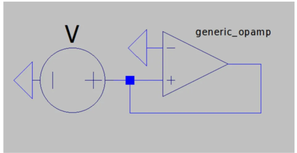
for closed-loop gain, as shown in Figure 2-4. Closed-loop gain relies on the output signal feeding back into the input in order to shape desired input. Op-amps that amplify through the use of closed-loop gain are less susceptible to voltage saturation through amplification. However, it should be noted that saturation can still occur through overvoltage from the input.

Figure 2-4: A generic op-amp with closed-loop gain.

2.1.3 Signal Amplification

The SXM uses a signal amplification chain to shape and condition x-ray flux signal for analog-to-digital conversion. Two different input configurations are discussed in this section, and select common amplification circuits are explained.

Inverting amplifiers take a positive DC voltage at the input and produce a larger negative voltage at the output. In AC amplification, the output is exactly 180 ∘ out of phase with the input. Non-inverting amplifiers take an AC input and preserve its phase in the amplified output. A positive voltage DC input will yield a positive voltage output.

The first common amplification circuit is a differentiator, shown in Figure 2-5. A differentiator is created using an inverting amplifier with a capacitor in the input line, and a resistor in the negative feedback loop, which can be considered a rudimentary high-pass filter. The differentiator output is proportional to the time derivative of

(34)

the input. The differentiator has a few characteristic limitations. For instance, a differentiator is susceptible to circuit noise is amplified in the output. A differentiator is also susceptible to high-frequency noise, causing instability [3].

Figure 2-5: An example differentiator circuit.

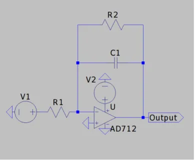
Similar to the differentiator, an integrator is used to integrate and invert an input signal. The output voltage is the time-dependent integral of the input voltage [3]. In this configuration, a resistor is included on the input line, and a capacitor is placed in the negative feedback loop, creating a low-pass filter, as shown in Figure 2-6.

In its simplest configuration, an integrator circuit requires periodic discharge of charge-saturated capacitors. When saturation occurs, the output voltage can drift beyond the optimal range of the op-amp. One way to mitigate this challenge is to include a resistor in the feedback loop that functions as a discharge path for the loop capacitor (Figure 2-7).

The last configuration used in the SXM is the Schmitt Trigger, which shapes an input signal into a square wave. An example Schmitt Trigger is provided in Figure 2-8. This configuration is used to shape a signal at a set voltage, to channel an input into a voltage accepted by the specifications of an analog-to-digital converter. A Schmitt Trigger is a modified integrator with positive feedback. A voltage divider is used to set the positive feedback, and looped back to the non-inverting input. When

(35)

Figure 2-6: An example integrator circuit.

Figure 2-7: An integrator circuit with an additional resistor added to the feedback loop provides a discharge path for the capacitor.

a prescribed threshold voltage is exceeded, the input voltage triggers and changes the state of the output voltage. This configuration is vulnerable to hysteresis effects. Schmitt Trigger hysteresis is dependent on resistance in the positive feedback loop. A Schmitt Trigger can operate as a binary switch. When a characteristic voltage is exceeded, the opamp drives the circuit output to the maximum voltage supplied by

(36)

the positive power rail. Below this characteristic voltage, feedback drives the opamp output to the minimum voltage connected on the negative power rail.

Figure 2-8: An example Schmitt Trigger.

2.1.4 Analog-to-Digital Signal Conversion

Analog-to-digital conversion is the process through which an analog signal is trans-lated into a series of digital values using an analog-to-digital converter (ADC). In the SXM, an input x-ray signal is amplified and shaped before being converted and digitized for data processing. The digital output from the ADC is proportional to the analog input signal, and is limited by quantization speed and accuracy concerns, where two signals detected in close succession might be amplified and captured as one signal. Quantization speed is critical for signal capture in instruments that receive rapid signal, or signal from multiple detectors at once. The SXM is a single diode detector, and does receive signal impulses close enough together to be concerned with quantization.

(37)

2.1.5 Thermal Impact on Circuitry

Temperature effects must be accounted for when designing and operating complex electrical systems. Amplification circuits often have a small window of acceptable input voltages, and signals must remain within specified bounds in order to be am-plified and ultimately converted by an ADC. An unexpected increase or decrease in temperature impacts part performance, signal suppression, and part longevity. Fur-thermore, unwanted over- or under-voltage can cause temporary or even irreversible damage to sensitive electrical systems.

The function of individual circuit elements is thermally dependent. For instance, an increase in temperature can affect power dissipation in resistors. Thermal condi-tions beyond a resistor’s rating causes permanent damage to the resistor by burning or melting internal materials. In capacitors, temperature can alter how charge moves within a dielectric material, increasing or decreasing the amount of charge required to saturate the component. Additionally, resistivity in the wiring connecting circuit elements scales positively with temperature and cause unintended voltages within the circuit.

Temperature concerns are considered in the design process of space hardware. For Class D missions, NASA recommends that only Level 1, Qualified Manufacturer List Class V (QMLV) legacy hardware is used in instrumentation. Circuitry tested to this level is rated for interplanetary spaceflight, where extreme radiation and thermal conditions are experienced [16]. The SXM was a "Do No Harm" instrument, and personnel working on the SXM received space rated electronics hardware and advice from design mentors at NASA Goddard Space Flight Center.1

2.2 SXM Overview

The SXM component of the REXIS instrument suite is a subassembly located on the OSIRIS-REx bus such that it faces the sun during windows of operation that REXIS

1_{Information from CAST interview with member of the SXM design team during CAST analysis}

(38)

is pointed at Bennu. The SXM is split into two parts, the SXM detector head and "backpack", and the MEB. The SXM detector head houses the SDD detector and the "backpack" contains the preamplification circuit. The "backpack" is connected to the SXM Main Electronics Board (MEB) by a coax tether. The SXM detector head mechanically adheres to the spacecraft bus using an aluminum mounting bracket. The SXM detector head is comprised of an Amptek XR-100SSD silicon drift diode (SDD) detector connected to a pre-amplification circuit (henceforth referred to as the preamp) located on a mounted printed circuit board (PCB).

When a solar x-ray hits the SDD detector, an analog signal is passed through the preamp, where it is conditioned and sent to the MEB. At the MEB, the analog signal passes through an ADC and captured as a digital response signal. This digital response is processed further by the MEB into x-ray energy event histograms sorted by energy level. Event energy data is kept in Analog-to-Digital Units, which can be converted to units of Electronvolt (eV). A conversion from ADU to eV is calculated using the formula

𝑘𝑒𝑉 = (0.0219 * 𝐴𝐷𝑈 ) + 𝑜𝑓 𝑓 𝑠𝑒𝑡, (2.8)

for the REXIS SXM.

Solar x-rays and their energies are then used to calculate the influx and energy of primary solar x-rays onto Bennu. A knowledge of primary x-ray energies is required to calibrate the secondary x-ray fluorescence capture by the REXIS detector.

2.3 SXM Data Pipeline

The SXM Data Pipeline takes a converted signal from the SXM ADC and processes it into data packets that are transmitted to the ground. The complete path for SXM signal through instrument response modeling and single temperature fitting is shown in Figure 2-9.

(39)

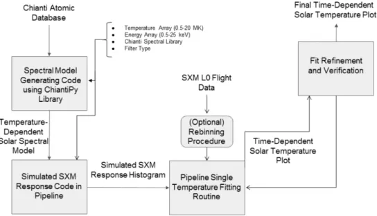
Figure 2-9: A spectral abundance model is created using the Chianti database. A simulated SXM response histogram shows instrument response based on the abun-dance model. Level 0 flight data from the SXM is matched to the simulated response histogram to generate single temperature fits and produce a time-dependent solar temperature plot.

2.3.1 Instrument Response Modeling

The SXM underwent a series of ground and in-flight validations between 2013 and 2019. This section focuses on the instrument response modeling used to verify early in-flight observations. The SXM Data Pipeline includes a model of ideal SXM response, which at its core captures a sample time-series of x-ray detections and produces energy histograms. These energy histograms are then fit to a known solar abundance model, which matches an input signal to x-ray characteristics of elements in the Sun’s photosphere, and subsequently constrain solar temperature at the time of x-ray emission. While this function fell beyond the original scope of the SXM’s purpose, it provided yet another way to produce instrument science.

2.3.2 Chianti Atomic Database

The Chianti Atomic Database creates an instrument response model across all tem-peratures and energies observable by the SXM. The Chianti Database is an atomic spectra database built and maintained by a global consortium of atomic scientists

(40)

[10]. Chianti and its associated python package, ChiantiPy, allow a user to generate model spectra of astrophysical bodies. For the purposes of the SXM, Chianti is a known database against which sample SXM histograms are matched. Both coronal and photospheric abundance models are generated at the temperatures and energies observable by the SXM, and ideal instrument response is cross-referenced against early in-flight calibration data taken prior to the REXIS instrument’s primary obser-vation window. Cross-referencing the Chianti database builds reasonable confidence in the instrument response model such that temperatures and spectra abundances are derived from data collected during observation.

2.4 CAST Analysis

This section provides an overview of CAST techniques applied to the SXM low x-ray count rate anomaly. A Causal Analysis based on System Theory (CAST) is an approach to accident investigation that adapts the System-Theoretical Accident Model and Process (STAMP) approach created at MIT by Dr. Nancy Leveson [13]. The CAST approach examines an accident, in this thesis the SXM low count rate anomaly, by constraining a system boundary around the incident, and includes a study of the culture, communication, and management of the project organization [14].

2.4.1 CAST Analysis Process

A CAST analysis is an impartial study of both the root cause of an accident and the key factors that created the environment in which the accident occurred [13]. Recommendations for improvements to future systems are provided to prevent future accidents. CAST utilizes personnel interviews to gain an understanding of who knew what, and when. The focus of CAST is to discover why an accident occurred, rather than direct any sort of blame [13],[14].

CAST incorporates a distinct vocabulary that allows the investigation to be ob-jective. Commonly used vocabulary include:

(41)

∙ A system goal is the objective of the system being examined.

∙ A system constraint is a condition in which the system goal can be met successfully.

∙ An accident is the undesired event that results in a loss.

∙ A loss is the result of an accident.

∙ A hazard is a condition or set of conditions in the project environment that allow the accident to occur.

2.4.2 Performing a CAST Analysis

A CAST Analysis is conducted in five steps:

∙ Acquire basic systems information

∙ Develop a safety control structure model

∙ Analyze individual loss components

∙ Identify systemic flaws in the control structure

∙ Provide recommendations for future systems

To begin a CAST analysis, information is gathered about the accident, loss, and associated hazards. A system boundary is created to maintain a directed investigative scope. The sequence of events is established and a set of general questions are com-piled [13]. A safety control structure is modeled. The safety control structure depicts various components within an organization, including organizational teams and the object to which the loss occurred. A safety control structure also depicts actions and influences as controls that did or did not create system hazards. An example safety control structure is shown in Figure 2-10.

Each component is examined individually to determine its role in in the timeline of events. Here, questions generated in the first step are answered, and further questions

(42)

Figure 2-10: An example safety control structure [13].

may be posed. In step four, key organizational interactions between components and overall organizational behavior are characterized based on information gathered in the previous step. The last step of the CAST analysis provides a set of recommendations for the current project team, as well as for similar future situations [14]. Feedback is given to the current team and events are documented thoroughly. A CAST analysis is ideal for the purpose of this thesis, because it investigates an unexpected result in solar x-ray data, and examines a dynamic organization that will serve as a model for future student spaceflight instruments.

(43)

Chapter 3 SXM Design and Operation

This chapter describes the design process and flight operations of the REXIS Solar X-ray Monitor (SXM). The first section will focus on the design constraints of the instrument. REXIS is a "Do No Harm" instrument on a Risk Class B mission which means it is a low budget instrument, and is designed to use legacy, off-the-shelf com-ponents [17],[18]. This section also describes the science requirements for the SXM, as well as comment on the lack of formal requirements prescribed by the OSIRIS-REx team, and how these requirements changed over time. The design section will primarily detail the development of the SXM signal amplification chain, which is at the center of the Root Cause investigation found in Chapter 4.

The next section of this chapter will describe ground testing used to characterize the SXM before launch. The SXM’s pre-flight ground testing regimen includes testing data relevant to the SXM root cause analysis, and include rationale for why some tests were foregone. Results of SXM in-flight calibration are presented, and nominal x-ray count data are shown.

The last section of this chapter summarizes SXM flight operations. A timeline of operations is included to understand where in-flight calibration occurred relative to science observations. Flight operations are separated into three distinct phases, which correlate to OSIRIS-REx mission phases. Early flight operations are described, followed by operations during Orbital B and Orbital R, REXIS’s two science operation phases.

(44)

3.1 SXM Design Background

The SXM was added to the REXIS project after the REXIS team had been awarded the student instrument contract by the OSIRIS-REx team in 2011. The SXM design team used heritage spaceflight technology. The SXM detector is an Amptek XR-100SDD, which is an updated model of the detectors flown on the NICER instrument. The XR-100SDD is an updated version of the XR-100CR, and the former uses a silicon drift diode, while the latter uses a PIN photodiode [1]. Both models have a beryllium window above an evacuated chamber in which the detector is housed. Amptek XR-100CR detectors were used in the Solar X-ray Spectrometer aboard GSAT-2, a space-based Indian solar observatory [6]. A similar Russian space observatory used the XR-100CR in the Solar Photometer in X-rays (SphinX) instrument [22]. Both of these previous instruments demonstrated that the Amptek XR-100 class detector could be reasonably be used to for x-ray solar observation, despite the XR-100SDD never having flown prior to REXIS.

The XR-100SDD detector was also included in early designs of the Neutron star Interior Composition ExploreR (NICER) instrument. NICER was developed by the MIT Kavli Institute (MKI), and the engineering teams worked closely together in the development processes. MIT Kavli Institute served as a Co-Investigator on the REXIS instrumet. The Goddard Spaceflight Center serves as the managing center for REXIS.

The NICER instrument is mounted aboard the International Space Station, where its main spectrometer observes neutron stars in the 0.2 to 12 keV range [5]. The REXIS SXM shares both structural and electronic heritage with the NICER instru-ment. An early design of NICER implemented 56 XR-100SDD detectors, the same detector used by the REXIS SXM. The NICER team later changed their design to use an Amptek CMOS detector, which benefits from higher temporal resolution.

While the NICER instrument and the REXIS SXM’s designs diverged during the design phase, the SXM was heavily influenced by this early NICER design. The de-sign of the SXM preamp circuit and SXM Electronics Board resemble the NICER

(45)

preamplifier board and surrounding electronics housing respectively. These similari-ties are the legacy of John Doty, an electrical engineer who consulted for the REXIS team and created the SXM timing circuitry, signal pulse shaping, and threshold trig-ger. These designs were further improved by Mike Jones, a graduate student working with the REXIS team from 2013-2015 [7]. A complete documentation of SXM circuit diagrams can be found in Appendix A.

3.1.1 Instrument Requirements

REXIS SXM requirements fall under the REXIS instrument’s main requirements, which in turn are derived from OSIRIS-REx requirements for the instrument. The REXIS requirements documentation flow was described extensively in Mike Jones’s Master’s thesis [7]. The information flow diagram for REXIS is shown in Figure 3-1

Figure 3-1: The REXIS Requirements documentation flow from Jones, 2015 [7].

The SXM’s energy band of interest is from 0.6 keV to 6 keV. Quantum efficiency for the SXM is also outlined in the REX-74 requirement. Quantum efficiency is the ratio of photon events that are successfully converted to electrons by the detector, and

(46)

is a metric used to evaluate the performance of an instrument at different detection energies (shown in Table 3.1).

Table 3.1: Quantum Efficiency Requirements for the SXM Detector.

Quantum Efficiency Energy Range (keV)

>0.01 0.62 - 0.7 >0.03 0.7 - 0.8 >0.09 0.8 - 1.2 >0.65 1.6 - 2.8 >0.85 2.8 - 4.1 >0.9 6.0 - 7.0

The REXIS SXM Requirements are derived from the different levels of REXIS requirements. The Level 2 requirement REX-7 is the highest-level requirement per-taining to the SXM. REX-7 requires that the SXM "shall measure solar coronal tem-perature to within 0.1 MK every 50 sec while observing Bennu in Phase 5B assuming a single temperature model." Level 3 documentation describes the requirements for detector functionality. SXM operational and environmental requirements are found in the Level 4 documentation. An important note is that the MEB had no temperature requirements during design. This contrasts with the SXM detector head and preamp were given temperature requirements. A complete overview of Level 3 and Level 4 requirements can be seen in Tables 3.2 and 3.3.

3.1.2 Overview of SXM Signal Amplification Chain

The SXM amplification chain is responsible for priming a signal from the SDD de-tector before it is converted by the Analog-to-Digital Converter (ADC). The amplifi-cation chain is housed on the SXM Main Electronics Board (MEB), which is located within the REXIS main spectrometer on the spacecraft. The SXM detector and preamp circuit are housed in the SXM backpack, which is connected to the outside of the spacecraft by the SXM bracket. The backpack houses both power and data for the detector, and is connected by a coax cable to the MEB. The SXM detector housing is shown in Figure 3-2.

(47)

Table 3.2: SXM Level 3 Requirements [7].

ID No. Title Description

REX-225 Integration

Time

The SXM shall integrate counts for 32 seconds (nominally) to form a spec-trum.

REX-73 Spectral

Resolu-tion

The SXM shall have a spectral resolu-tion (FWHM) that is less than 200 eV from 0.6 to 6 keV.

REX-74 Quantum

Effi-ciency

The SXM shall detect x-ray events from 0.6 to 6.0 keV with quantum efficiencies as given in Table 3.1.

REX-75 Field of View The SXM shall have a full width zero

intensity (FWZI) FOV of no greater than 60 deg full cone and a full width full intensity (FWFI) FOV of no less than 10 deg full cone.

Table 3.3: SXM Level 4 Requirements [7].

ID No. Title Description

REX-228 SDD Survival

Temperature

The temperature of the SDD shall al-ways be greater than -65∘C and less than 150∘C.

REX-229 SDD Operating

Temperature

The temperature of the SDD shall be less than -30∘Cand greater than -70∘C.

REX-76 Preamp Survival

Temperature

The temperature of the SXM Preamp shall be greater than -55∘C and less than 85∘C.

REX-77 Preamp

Operat-ing Temperature

The temperature of the SXM preamp shall be greater than -40∘C and less than 85∘C while operating.

REX-78 SXM Health The SXM shall survive and remain

op-erational through the end of Phase 8.

REX-79 SXM

Opera-tional Time

The SXM shall be capable of operating 24 hours per day

The SXM ADC requires a positive voltage signal pulse to be passed to it in order to register a detection count. Figure 3-3 provides an overview of SXM Signal processing. When an x-ray strikes the SDD detector, the measure of the incoming x-ray creates ionization within the detector’s silicon diode that in turn induces a charge in the form of a pulse signal. The raw signal is shaped in the preamp and then sent across

(48)

Figure 3-2: SXM detector and preamp housing. The SXM detector is located below the collimator.

Figure 3-3: A simple block diagram of SXM signal processing.

a coax cable to the MEB. When the signal reaches the MEB, it is passed through three opamps, which amplify the signal. Then the voltage signal is divided, such that one signal passes through an integrator circuit and the other signal through a differentiator circuit. The output from the integrator circuit is labeled outu, and the output from the differentiator circuit is labeled outb. The amplification chain schematic diagram is shown in Figure 3-4. Additional SXM electronics schematics can be found in Appendix A.

(49)

Figure 3-4: Sc hematic of SXM Amplification Chain. Outputs outb and outu are seen on the far righ t. The Outb opamp is configured as a differen tiator circuit, a n d the outb opamp is co n figured as an in tegrator circuit. The three opamps b ehind the outu and outb opamps amplify the signal from the preamp.

(50)

noise artifacts added to the signal when it passed through the preamp circuit. The outu signal is then sent to the final section of the amplification circuit, where 3 V of bias are subtracted, leaving the signal with a residual 0.3 V bias. This bias is required to keep the outu signal positive because the ADC used in the SXM electronics chain is not rated for negative voltage inputs. When the bias subtraction occurs, outu becomes 𝑜𝑢𝑡𝑢1. Subtracting the outu bias prevents 𝑜𝑢𝑡𝑢1 from reaching high signal

saturation.

Next, Signal outu is sent to the ADC to be measured, while signal outb is sent to a zero cross monitor, that provides the timing for the ADC to sample new signal, now named outu1.

In order to trigger an ADC detection, the SXM relies on a trigger circuit that uses a series of comparators to compare outb to a reference voltage. The trigger circuit is shown in Figure 3-5.

This trigger includes a command to manually set the threshold Voltage Lower Limit of Detection (VLLD). The VLLD is set above the outb bias voltage as well as the noise floor to prevent the SXM from accidentally triggering due to random noise in the electronics. The relationship of outb to VLLD is considered a binary switch

⎧ ⎪ ⎨ ⎪ ⎩ 𝑉 𝐿𝐿𝐷 > 𝑜𝑢𝑡𝑏 𝐿𝐿𝐷 = 0 𝑉 𝐿𝐿𝐷 < 𝑜𝑢𝑡𝑏 𝐿𝐿𝐷 ≈ 2.4𝑉

where LLD is the Lower Limit of Detection.

The second threshold circuit is used to determine the zero crossing of outb. When 𝑜𝑢𝑡𝑢1 is at it’s peak, outb will have a zero crossing with the outb nominal voltage,

and the ADC is triggered to begin recording [2]. Figure 3-6 shows an example of all signal shapes.

3.2 Instrument Level Testing

As part of the instrument design process, the REXIS SXM was subject to numer-ous functionality tests on the ground. Testing was limited by time and financial

(51)

Figure 3-5: SXM Trigger Circuit Schematic. When outb exceeds VLLD, LLD switches from 0 V to its on state at 2.4V. LLD’s rising action arms the ADC for detection. In the top comparator, when VB exceeds outb, ZP switches from its on setting to 0 V. ZP’s change of state tells the ADC to trigger, and coincides with the maximum of 𝑜𝑢𝑡𝑢1.

(52)

Figure 3-6: SXM signals at various points throughout the amplification chain [7]. outu is the output signal from the integrator circuit, and 𝑜𝑢𝑡𝑢1 is outu minus an offset

voltage. Outb is the output of the differentiator circuit. When outb exceeds VLLD, LLD goes high, arming the ADC. As outb falls below VLLD, LLD returns to 0 V. The zero point of outb where it crosses its steady state voltage coincides with the peak of 𝑜𝑢𝑡𝑢1. When 𝑜𝑢𝑡𝑢1 is at its maximum, ZP switches states and triggers the

ADC. The peak height of 𝑜𝑢𝑡𝑢1 is captured by the ADC and provides the energy of

the x-ray being detected.

constraints, but the testing framework was rigorous and proved the SXM ready for flight. The subsection on ground testing focuses on testing that provided thermal

(53)

testing history for the SXM, which is important for investigating the SXM low count rate anomaly discussed in Chapter 4. A more thorough description of SXM ground testing can be found in Kevin Stout’s thesis [21].

The SXM also underwent a series of in-flight calibrations between launch in 2016 and Orbital B, the first data collection phase, in July of 2019. Flight testing was pri-marily used to characterize the REXIS main spectrometer, whose CCD array required in-flight calibration, and the SXM was tested as well [9].

3.2.1 Ground Testing

The SXM flight model was put through a battery of ground tests to ensure the in-strument was working properly and ready for launch. The testing procedure followed NASA requirements for Risk Class B missions and were optional for the REXIS SXM, which was classified as a "Do No Harm" instrument [17]. The focus of this subsection is on SXM thermal tests, which provide a background for the root cause analysis outlined in Chapter 4.

The SXM flight model was subject to thermal testing using thermal vacuum cham-bers built in the MIT Space Systems Laboratory and at MIT Lincoln Laboratory in Fall 2015. Environmental testing was conducted by the REXIS team at the Applied Physics Laboratory in the summer of 2015.

SXM Flight Model Delivery and Early Repairs

The SXM flight model was delivered in June 2015. A number of issues are identified: the first of which concerns the TEC cooling unit power supply which, due to a change to rad-hard optocouples, does not regulate voltage appropriately and exceeds maxi-mum allowable voltages in the device. To remedy the TEC power issue and another error in the cable-diagram / MEB pinout to the SXM the backpack board is created which creates a feedthrough that corrects the pinout issue. A power supply board within the backpack is designed to supply power directly to the TEC and the MEB. This was altered for both the flight spare and the flight model to accommodate this.

(54)

The only change was the removal of the optocopyles. Following the repair of the TEC, testing of the SXM could be directly carried out on the flight spare and MEB but it was determined that the flight spare was still not triggering on X-ray events although the pre-amplifier could be seen at the input into the electronics. After the application of a conformal coating to protect the MEB, alterations of this nature were more difficult. After these repairs, the SXM still did not function. Further repairs were identified, but were deferred to after environmental testing, while the possibility of science without the SXM was discussed.

Environmental Testing

REXIS underwent environmental testing at the Applied Physics Laboratory (APL) in August 2015. The SXM flight model was not functioning during environmental testing. The main spectrometer demonstrated an issue with the degradation of energy resolution during environmental testing.

REXIS at Lockheed Martin

The solution for the degradation of energy resolution in the main spectrometer was identified, and the REXIS instrument returned to MIT for a few weeks and underwent

a pre-ship review during this time. REXIS was supposed to be mounted to the

spacecraft when it was delivered to Lockheed Martin. However, at Lockheed Martin results from a vibration test conducted at APL raised structural concerns and REXIS was returned to MIT.

SXM Instrument Level Testing

In October 2015, the REXIS main spectrometer underwent electrical repairs that corrected previous issues. The SXM was functional, although a threshold anomaly was discovered. Members of the REXIS team identified a fix to the threshold startup sequence that fixed threshold control. The threshold anomaly fix involved setting the SXM trigger threshold to its maximum voltage twice before setting the threshold at the desired voltage.

(55)

Next, the SXM underwent instrument level testing at Lincoln Laboratory in November 2015. The SXM detector head, preamp board, and MEB were placed in a thermal vacuum (TVAC) chamber. The temperature of the thermal chamber was then cycled between -40∘C and 60∘C with a ground calibration Fe-55 x-ray source to measure instrument performance as a function of temperature. An example histogram from the ground calibration source is shown in Figure 3-7.

Figure 3-7: A calibration histogram showing SXM response to an Fe-55 source.

Varying temperature in both the preamp and MEB produced a gain change and indicated thermal sensitivity in the SXM. The Preamp and the MEB had separate heaters during the instrument level test, and gain changes seemed to correlate more with thermal changes in the MEB than in the Preamp.

As the MEB temperature increased, the SXM recorded lower source counts than at lower temperatures. Hysteresis effects were also seen in the MEB, and it was determined that temperature changes in the MEB can result in changes to the SXM’s low energy threshold. The results of the instrument level test are provided in Figure

(56)

Figure 3-8: Set temperatures on the DE during Instrument Level TVAC Test, 2015. The DE is considered a proxy for MEB temperature because the DE records all boards housed in the REXIS Electronics Box where the MEB resides. The DE records lower temperature noise than the MEB, making the DE temperature sensor a more accurate measurement.

3-9.

Figure 3-9: Instrument level testing results demonstrate a susceptibility in the MEB. The temperature recorded in this figure is of the MEB base plate and shows how temerature was cycled during the test.

Characterization of solar X-ray response data from the REXIS instrument

Characterization of Solar X-ray Response Data from the

REXIS Instrument

by

Andrew T. Cummings

Abstract

Acknowledgments

Contents

List of Figures

List of Tables

Chapter 1

Introduction

1.1

REXIS Mission

1.2

REXIS Operational Timeline

1.3

Motivation

1.4

Thesis Roadmap

Chapter 2

Background

2.1

Basic Circuitry

2.1.1

Common Components

2.1.2

Operational Amplifiers

2.1.3

Signal Amplification

2.1.4

Analog-to-Digital Signal Conversion

2.1.5

Thermal Impact on Circuitry

2.2

SXM Overview

2.3

SXM Data Pipeline

2.3.1

Instrument Response Modeling

2.3.2

Chianti Atomic Database

2.4

CAST Analysis

2.4.1

CAST Analysis Process

2.4.2

Performing a CAST Analysis

Chapter 3

SXM Design and Operation

3.1

SXM Design Background

3.1.1

Instrument Requirements

3.1.2

Overview of SXM Signal Amplification Chain

3.2

Instrument Level Testing

3.2.1

Ground Testing