Optical in situ and geostationary satellite-borne observations of suspended particles in coastal waters

HAL Id: tel-02178385

https://tel.archives-ouvertes.fr/tel-02178385

Submitted on 9 Jul 2019

HAL is a multi-disciplinary open access archive for the deposit and dissemination of sci-entific research documents, whether they are pub-lished or not. The documents may come from teaching and research institutions in France or abroad, or from public or private research centers.

L’archive ouverte pluridisciplinaire HAL, est destinée au dépôt et à la diffusion de documents scientifiques de niveau recherche, publiés ou non, émanant des établissements d’enseignement et de recherche français ou étrangers, des laboratoires publics ou privés.

observations of suspended particles in coastal waters

Griet Neukermans

To cite this version:

Griet Neukermans. Optical in situ and geostationary satellite-borne observations of suspended par-ticles in coastal waters. Oceanography. Université du Littoral Côte d’Opale, 2012. English. �NNT : 2012DUNK0406�. �tel-02178385�

T

HÈSE

D

E L

’U

NIVERSITÉ DU

L

ITTORAL

C

OTE D

’O

PALE

La oratoire d’O a ologie et de G os ie es

Présentée par Griet NEUKERMANS

Pour obtenir le grade de Docteur en Sciences de la Mati re, du Rayo e e t et de l’E viro e e t

Spécialité Océanographie

Sujet de thèse

Les particules en suspension dans les eaux côtières turbides:

esti atio pa esu es opti ues i situ et depuis l’espace

Soutenue le 18 avril 2012

devant le jury composé de

Directeur de thèse Hubert

L

OISEL (LOG, France)

Co-Directeur de thèse Kevin

R

UDDICK (MUMM, Belgique)

Rapporteurs David

A

NTOINE (LOV, France)

Michael

T

WARDOWSKI (WET Labs, USA)

Membres de jury Jean-François

B

ERTHON (JRC, Italy)

Emmanuel

B

OSS (UMaine, USA)

D

ISSERTATION

U

NIVERSITÉ DU

L

ITTORAL

C

OTE D

’O

PALE

La oratoire d’O a ologie et de G os ie es

By Griet

N

EUKERMANS

Submitted in partial fulfillment of the requirements for the degree of Doctor in Science (Oceanography)

Subject

Optical in situ and geostationary

satellite-borne observations of

suspended particles in coastal waters

Defended on 18 April 2012

for the dissertation committee composed of

Promoter Hubert

L

OISEL (LOG, France)

Co-Promoter Kevin

R

UDDICK (MUMM, Belgium)

Reporters David

A

NTOINE (LOV, France)

Michael

T

WARDOWSKI (WET Labs, USA)

Committee members Jean-François

B

ERTHON (JRC, Italy)

Emmanuel

B

OSS (UMaine, USA)

Print: Silhouet, Maldegem

© 2012 Griet Neukermans

2012 ASP nv (Academic and Scientific Publishers nv)

Ravensteingalerij 28

B-1000 Brussel

Tel. + 32 (0)2 289 26 50

Fax + 32 (0)2 289 26 59

info@aspeditions.be

www.aspeditions.be

ISBN 978 90 7028 949 2

NUR 912

Legal deposit D/2012/11.161/015

All rights reserved. No parts of this book may be reproduced or transmitted in any form or by

any means, electronic, mechanical, photocopying, recording, or otherwise, without the prior

written permission of the author.

This thesis work was funded by the Belgian Science Policy Office (BELSPO) STEREO

Programme in the framework of the BELCOLOUR-2 (SR/00/104) and GEOCOLOUR

(SR/00/139) projects.

This work was also supported by Centre National d’Etude Spatiale

(CNES) in the frame of the COULCOT project (TOSCA program).

Keywords: diurnal variability, tidal variability, resuspension, PAR attenuation, particulate

scattering coefficient, bio-optics, particle size distribution, mass-specific scattering coefficient,

light attenuation, turbidity, suspended particulate matter concentration measurement protocol,

ocean colour, remote sensing, atmospheric correction, meteorological satellite, SEVIRI, MODIS.

C

ONTENT

Acknowledgements i

Abstract ii

Résumé iii

Samenvatting v

List of abbreviations and acronyms vii

List of symbols xi

List of Figures xvii

List of Tables xxvii

GENERAL INTRODUCTION 1

CHAPTER 1 OPTICAL PROPERTIES AND SEAWATER CONSTITUENTS: DEFINITIONS

AND MEASUREMENT 5

1.1 SEAWATER CONSTITUENTS 5

1.2 OPTICAL PROPERTIES 7

1.2.1 INHERENT OPTICAL PROPERTIES (IOPS) 8

1.2.1.1 Definition of IOPs 8

1.2.1.2 Partitioning of IOPs 10

1.2.1.3 Concentration-specific IOPs 11

1.2.2 APPARENT OPTICAL PROPERTIES (AOPS) 12

1.2.2.1 Reflectances 13

1.2.2.2 Diffuse attenuation coefficients 14

1.2.3 LINK BETWEEN IOPS AND AOPS 15

1.3.1 IOPS 16

1.3.1.1 Beam attenuation 16

1.3.1.2 Combined measurements of absorption and attenuation 18

1.3.1.3 Volume scattering function and backscattering coefficients 19

1.3.1.4 Turbidity 20

1.3.2 AOPS 21

1.3.2.1 Above-water radiometry 21

CHAPTER 2 TURBIDITY MEASUREMENTS TO OPTIMIZE MEASUREMENTS OF

SUSPENDED PARTICULATE MATTER CONCENTRATION 25

ABSTRACT 25

2.1 INTRODUCTION 25

2.2 MATERIALS AND METHODS 27

2.2.1 MEASUREMENT OF [SPM] 27

2.2.1.1 Measurement protocol 27

2.2.1.2 Filter blanks 28

2.2.1.3 Salt retention tests 29

2.2.2 TURBIDITY MEASUREMENTS 29

2.2.3 OPTIMAL FILTRATION VOLUME 30

2.2.3.1 T as proxy for [SPM] 30

2.2.3.2 Determining optimal filtration volume 30

2.2.4 EFFECT OF FILTRATION VOLUME ON PRECISION OF [SPM] MEASUREMENTS 31

2.2.5 BETWEEN GROUP STATISTICAL ANALYSIS 31

2.3 RESULTS AND DISCUSSION 32

2.3.1 UNCERTAINTIES IN [SPM] MEASUREMENT 32

2.3.1.1 Salt retention tests 32

2.3.1.2 Filter blanks 33

2.3.1.3 Sample mixing 34

2.3.2 UNCERTAINTIES IN [SPM] MEASUREMENT FROM FILTRATION VOLUME 35

2.3.2.1 Determining optimal filtration volume 35

2.3.2.2 Effect of filtration volume on precision of [SPM] measurement 39

BACKSCATTERING OF MARINE PARTICLES WITH RESPECT TO PARTICLE SIZE,

DENSITY, AND COMPOSITION 45

ABSTRACT 45

3.1 INTRODUCTION 45

3.2 METHODS 49

3.2.1 DESCRIPTION OF THE STUDY AREAS 49

3.2.2 OPTICAL MEASUREMENTS 51

3.2.3 WATER SAMPLING 54

3.2.4 PARTICLE SIZE AND MEAN APPARENT DENSITY 55

3.2.5 MASS-SPECIFIC ATTENUATION AND BACKSCATTERING COEFFICIENTS 57

3.3 RESULTS 59

3.3.1 INSTRUMENT INTERCOMPARISON FOR PARTICULATE BEAM ATTENUATION 59

3.3.2 RELATIONSHIPS BETWEEN SCATTERING PROPERTIES AND PARTICLE CONCENTRATION BY AREA OR

DRY WEIGHT 61

3.3.3 INVESTIGATION OF THE VARIABILITY OF MASS-SPECIFIC SCATTERING PROPERTIES 64 3.3.4 INVESTIGATION OF THE VARIABILITY OF ATTENUATION AND BACKSCATTERING EFFICIENCY 70

3.3.5 SCATTERING MEASUREMENTS AS PROXIES FOR [SPM] 73

3.4 DISCUSSION AND CONCLUSION 75

3.5 APPENDICES 79

3.5.1 DEALING WITH MEASUREMENT UNCERTAINTIES: PROPAGATION OF UNCERTAINTIES AND LINEAR

REGRESSION METHODS 79

3.5.1.1 Repeat measurements of IOPs and particle concentration 79

3.5.1.2 Propagation of uncertainty 80

3.5.1.3 Least squares regression for measurements with uncertainties 82

3.5.1.4 Correlation coefficient uncertainty estimation 84

3.5.2 IOPS AND PARTICLE SIZE DISTRIBUTIONS 84

3.5.2.1 Scattering properties vs. area concentration by size class 84

3.5.2.2 Particle size distributions 89

3.5.2.3 Relationship between Junge PSD slope and cp spectral slope from in situ measurements 91

ABSTRACT 95

4.1 INTRODUCTION 96

4.2 MATERIALS AND METHODS 98

4.2.1 THE SEVIRI RADIOMETER 98

4.2.2 STUDY AREA:SEVIRI SUBSCENE AND VIEWING ANGLES 100

4.2.3 DEFINITIONS AND GENERAL APPROACH 102

4.2.4 SEVIRI SOLAR CHANNELS CALIBRATION 106

4.2.5 ATMOSPHERIC CORRECTION OF SEVIRIVIS06 107

4.2.5.1 Rayleigh and gas corrections 107

4.2.5.2 Aerosol correction 108

4.2.5.3 Atmospheric correction assumptions 109

4.2.5.4 Solving for marine and aerosol reflectances 113

4.2.5.5 Atmospheric correction processing steps 114

4.2.6 ATMOSPHERIC CORRECTION USING THE HRV BAND 115

4.2.6.1 Relating marine reflectances in the HRV and VIS06 bands 115

4.2.6.2 Estimating spatial variability of



_w0(0.6) on the HRV grid from HRV spatial anomaly 117

4.2.7 ESTIMATE OF UNCERTAINTY ON MARINE REFLECTANCE 118

4.2.7.1 Uncertainties associated with the atmospheric correction assumptions 118

4.2.7.2 Digitization uncertainties 119

4.2.7.3 Combined atmospheric-digitization uncertainty 120

4.2.7.4 Uncertainty estimate of marine reflectance in the VIS06 band on the HRV grid 122

4.2.8 CROSS-VALIDATION WITH MODIS REFLECTANCE DATA 122

4.3 RESULTS 124

4.3.1 MAPPING MARINE REFLECTANCE AND ITS UNCERTAINTIES 124

4.3.2 MARINE REFLECTANCE ON THE HRV GRID 125

4.3.3 SEVIRI–MODIS CROSS VALIDATION 126

4.3.3.1 VIS06 reflectance 126

4.3.3.2 VIS06 reflectances on the HRV grid 130

4.3.4 DIURNAL VARIABILITY OF MARINE REFLECTANCES AND AEROSOLS 131

4.4 DISCUSSION AND CONCLUSION 133

4.4.1 OPTIMAL REFLECTANCE RANGE FOR ATMOSPHERIC CORRECTION 133

4.4.2 SPATIAL RESOLUTION 135

4.4.3 EXPLOITING HIGH TEMPORAL RESOLUTION IMAGERY 136

4.5.1 COMPARISON OF BANDS VIS08 AND NIR16 FOR AEROSOL CORRECTION OF VIS06 139 4.5.1.1 Estimation of uncertainty on



_w0(0.6) using band combination (VIS06, NIR16) 139 4.5.1.2 Band pair selection based on minimization of





_w0(0.6) 141 4.5.2 INTER-CALIBRATION OF VIS06 AND VIS08 BANDS USING RAYLEIGH AND GAS-CORRECTED

REFLECTANCES 142

CHAPTER 5 DIURNAL VARIABILITY OF TURBIDITY AND LIGHT ATTENUATION IN TURBID SOUTHERN NORTH SEA WATERS FROM THE SEVIRI GEOSTATIONARY

SENSOR 145

ABSTRACT 145

5.1 INTRODUCTION 145

5.2 MATERIALS AND METHODS 146

5.2.1 RETRIEVAL OF TURBIDITY AND SUSPENDED MATTER FROM SEVIRI 146

5.2.1.1 Retrieval Algorithms 146

5.2.1.2 Uncertainty on SEVIRI turbidity and suspended matter products 147

5.2.2 RETRIEVAL OF PAR ATTENUATION 148

5.2.2.1 PAR attenuation algorithm 148

5.2.2.2 Uncertainty on PAR attenuation retrieval 149

5.2.3 VALIDATION OF SEVIRI TURBIDITY AND PAR ATTENUATION PRODUCTS 149

5.2.3.1 SmartBuoy measurements of turbidity and PAR attenuation 149

5.2.3.2 Comparison of instantaneous SEVIRI-SmartBuoy observations 150

5.2.3.3 Validation of SEVIRI product time series 150

5.3 RESULTS 151

5.3.1 COMPARISON OF INSTANTANEOUS SEVIRI-SMARTBUOY OBSERVATIONS 151

5.3.1.1 Turbidity observations 151

5.3.1.2 PAR attenuation observations 151

5.3.2 VALIDATION OF SEVIRI PRODUCT TIME SERIES 155

5.3.2.1 Time series of turbidity 155

5.3.2.2 Times series of PAR attenuation 158

5.4 DISCUSSION 160

5.4.2 LIMITATIONS OF SEVIRI SPATIAL RESOLUTION 162

5.4.2.1 sub-pixel scale variability 162

5.4.2.2 Use of the HRV band 164

5.4.3 LIMITATIONS OF THE T AND KD RETRIEVAL ALGORITHMS 164

5.4.3.1 Turbidity retrieval algorithm 164

5.4.3.2 KPAR retrieval algorithm 164

5.4.4 INCOMMENSURABILITY BETWEEN IN-SITU AND REMOTELY SENSED PRODUCTS 165

5.4.4.1 remotely sensed vs. in-situ T 165

5.4.4.2 Remotely sensed vs. in-situ KPAR 166

5.4.5 PERSPECTIVES FOR THE DESIGN OF FUTURE GEOSTATIONARY SENSORS AND SYNERGY WITH

POLAR-ORBITING SENSORS 167

5.5 CONCLUSION 168

5.6 APPENDICES 168

5.6.1 CALIBRATION DATASET FOR TURBIDITY AND [SPM] RETRIEVAL ALGORITHMS 168

5.6.1.1 Data collection, treatment, and selection 169

5.6.1.2 Impact of [SPM] measurement improvement on the [SPM] retrieval algorithm 170

5.6.2 VARIABILITY OF TURBIDITY-SPECIFIC BACKSCATTERING 171

5.6.3 UNCERTAINTIES OF THE T AND [SPM] RETRIEVAL ALGORITHMS 173

5.6.3.1 Variability of the mass- and turbidity-specific backscattering coefficient 173

5.6.3.2 regional calibration 175

5.6.4 COUPLING BETWEEN TURBIDITY AND HYDRODYNAMICS 175

CHAPTER 6 GENERAL CONCLUSIONS AND PERSPECTIVES 179

6.1 IN-SITU VARIABILITY OF SCATTERING PROPERTIES AND SUSPENDED MATTER CONCENTRATION 179 6.2 REMOTE SENSING OF DIURNAL VARIABILITY OF SUSPENDED PARTICLES FROM THE

GEOSTATIONARY SEVIRI METEOROLOGICAL SENSOR 180

REFERENCES 185

A

CKNOWLEDGEMENTS

This dissertation is the result of collaboration between the Laboratoire d’Océanographie et de Géosciences (LOG) and the Management Unit of the North Sea Mathematical Models (MUMM). I am very grateful to the numerous people who contributed to this work.

My foremost gratitude to my promoter and co-promoter, Hubert Loisel and Kevin Ruddick, for their guidance, mentoring, and support. I was a lucky pupil to have learned from the masters in marine optics and atmospheric correction!

I thank the reporters of my dissertation, David Antoine and Mike Twardowski, and members of the dissertation committee, Jean-François Berthon, Emmanuel Boss, and François Schmitt for evaluating and reviewing this work.

Many thanks to my colleagues of the Remote Sensing and Ecosytem Modeling team of MUMM and of the Physical Oceanography, Transport, and Remote Sensing team of LOG. I received a great deal of support and assistance of a few people in particular: Xavier Mériaux for data processing and lab analysis, Lucie Courcot for Electron Microscopy analysis, Clémence Goyens for translating the abstract, Michel Laréal for technical support, Quinten Vanhellemont for providing ocean colour data, Geneviève Lacroix for hydrodynamic modeling, and Bouchra Nechad for suspended matter retrieval algorithms.

The crews of research vessels Belgica, Alliance, Papy Jo, and Zeeleeuw are thanked for their kind help during many sea campaigns. Thanks to the Chemistry Laboratory of MUMM for their analysis of hundreds of suspended matter and phytoplankton pigment samples. I also thank Flanders Marine Institute (VLIZ) for providing a LISST instrument during several campaigns.

I am very grateful to Nicolas Clerbaux of the Royal Meteorological Institute of Belgium for providing SEVIRI data and kind support. Thanks to Naomi Greenwood of the Centre for Environment, Fisheries & Aquaculture Science, for providing SmartBuoy data and kind help.

Thanks to the BELCOLOUR-2 and GEOCOLOUR project scientists and steering committee members for scientific discussions and data sharing.

Finally, a special thanks to my parents, Peter and Jelle, for giving me the chance to study, develop, and grow, and for their trust, love, and support. Many thanks to my family and friends for their love and understanding.

A

BSTRACT

Particles suspended in seawater include sediments, phytoplankton, zooplankton, bacteria, viruses, and detritus, and are collectively referred to as suspended particulate matter, SPM. In coastal waters, SPM is transported over long distances and in the water column by biological, tide or wind-driven advection and resuspension processes, thus varying strongly in time and space. These strong dynamics challenge the traditional measurement of the concentration of SPM, [SPM], through filtration of seawater sampled from ships. Estimation of [SPM] from sensors recording optical scattering allows to cover larger temporal or spatial scales. So called ocean colour satellites, for example, have been used for the mapping of [SPM] on a global scale since the late 1970s. These polar-orbiting satellites typically provide one image per day for the North Sea area. However, the sampling frequency of these satellites is a serious limitation in coastal waters where [SPM] changes rapidly during the day due to tides and winds. Optical instruments installed on moored platforms or on under-water vehicles can be operated continuously, but their spatial coverage is limited. This work aims to advance in situ and space-based optical techniques for [SPM] retrieval by investigating the natural variability in the relationship between [SPM] and light scattering by particles and by investigating whether the European geostationary meteorological SEVIRI sensor, which provides imagery every 15 minutes, can be used for the mapping of [SPM] in the southern North Sea.

Based on an extensive in situ dataset, we show that [SPM] is best estimated from red light scattered in the back directions (backscattering). Moreover, the relationship between [SPM] and particulate backscattering is driven by the organic/inorganic composition of suspended particles, offering opportunities to improve [SPM] retrieval algorithms. We also show that SEVIRI successfully retrieves [SPM] and related parameters such as turbidity and the vertical light attenuation coefficient in turbid waters. Even though uncertainties are considerable in clear waters, this is a remarkable result for a meteorological sensor designed to monitor clouds and ice, much brighter targets than the sea! On cloud free days, tidal variability of [SPM] can now be resolved by remote sensing for the first time, offering new opportunities for monitoring of turbidity and ecosystem modelling. In June 2010 the first geostationary ocean colour sensor was launched into space which provides hourly multispectral imagery of Korean waters. Other geostationary ocean colour sensors are likely to become operational in the (near?) future over the rest of the world’s seas. This work allows us to maximally prepare for the coming of geostationary ocean colour satellites, which are expected to revolutionize optical oceanography.

R

ÉSUMÉ

Les particules en suspension dans l'eau de mer incluent les sédiments, le phytoplancton, le zooplancton, les bactéries, les virus, et des détritus. Ces particules sont communément appelés matière en suspension (MES). Dans les eaux côtières, la MES peut parcourir de longues distances et être transportée verticalement à travers la colonne d'eau sous l'effet des vents et des marées favorisant les processus d'advection et de resuspension. Ceci implique une large variabilité spatio-temporelle de MES et quasiment impossible à reconstituer à travers les mesures traditionnelles des concentrations de MES, [MES], par filtration de l'eau de mer à bord de bateaux. La [MES] peut être obtenue à partir de capteurs optiques enregistrant la diffusion et déployés soit de manière in-situ, soit à partir d'un satellite dans l'espace. Depuis la fin des années 70, par exemple, les satellites « couleur de l'eau » permettent d'établir des cartes de [MES] globales. La fréquence d’une image par jour pour la mer du Nord de ces capteurs polaires représente un obstacle non-négligeable pour l'étude de variabilité de la [MES] dans les eaux côtières où la marée et les vents engendrent des variations rapides au cours de la journée. Cette limitation est d'autant plus importante pour les régions avec une couverture nuageuse fréquente. Les méthodes in-situ à partir d’un navire autonome ou d'une plateforme amarrée permettent d'enregistrer des données en continu mais leur couverture spatiale reste néanmoins limitée. Ce travail a pour objectif de mettre en avant les techniques de mesures in-situ et satellites de la [MES] en se concentrant principalement sur deux points. Premièrement, d’acquérir une meilleure connaissance de la variabilité de la relation entre la [MES] et la lumière diffuse, et deuxièmement, d’établir des cartes de [MES] dans la mer du Nord avec le capteur géostationnaire météorologique Européen (SEVIRI), qui donne des images chaque 15 minutes.

La variabilité de la relation entre la [MES] et la lumière diffuse est étudiée à l'aide d'une banque de données in-situ. Nous démontrons que la [MES] est le mieux estimée à partir des mesures dans l'intervalle rouge du spectre de lumière rétro-diffuse. Par ailleurs, la relation entre la [MES] et la rétrodiffusion est gouvernée par la composition organique/inorganique des particules, ce qui représente des possibilités d'amélioration pour les algorithmes d'estimation de [MES] à partir de la couleur de l'eau. Nous démontrons aussi qu’avec SEVIRI il est possible d’estimer la [MES], la turbidité et le coefficient d'atténuation, deux variables étroitement liées à la [MES], avec généralement une bonne précision. Bien qu'il y ait d'importantes incertitudes dans les eaux claires, cette réussite est remarquable pour un capteur météorologique initialement conçu pour le suivi des nuages et des masses glacières, cibles beaucoup plus brillantes que la mer! Ce travail démontre pour la première fois que la variabilité de la [MES] à l'échelle temporelle des marées dans les eaux côtières au sud de la Mer du Nord peut être capturée et mesurée par le biais de la télédétection de la couleur de l'eau ; ce qui ouvre des opportunités pour le monitoring de la

turbidité et pour la modélisation des écosystèmes. Le premier capteur géostationnaire couleur de l’eau à été lancé en juin 2012, donnant des images multispectrale des eaux coréennes chaque heure. D’autres capteurs vont probablement suivre dans l’avenir (proche ?), couvrant le reste des eaux du globe. Ce travail nous permet de préparer, de façon optimale, l’arrivée de ces capteurs qui vont révolutionner l'océanographie optique.

S

AMENVATTING

De in zeewater aanwezige zwevende materie zoals sedimenten, fytoplankton, zooplankton, bacteriën, virussen en detritus, worden collectief “suspended particulate matter” (SPM) genoemd. In kustwateren worden deze deeltjes over lange afstanden en in de waterkolom getransporteerd door biologische processen of wind- of getijdenwerking, waardoor SPM sterk varieert in ruimte en tijd. Door deze sterke dynamiek wordt de traditionele bemonstering van de concentratie van SPM, [SPM], door middel van filtratie van zeewaterstalen aan boord van schepen ontoereikend. Optische technieken die gebruik maken van de lichtverstrooiingseigenschappen van SPM bieden een gebieds- of tijdsdekkend alternatief. Zogenaamde “ocean colour” satellieten bijvoorbeeld leveren beelden van o.a. [SPM] aan het zeeoppervlak op globale schaal sinds eind 1970, met een frequentie van één beeld per dag voor de Noordzee. Deze frequentie is echter onvoldoende in onze kustwateren waar [SPM] drastisch kan veranderen in enkele uren tijd. Optische instrumenten aan boord van schepen of op onderwatervoertuigen kunnen continu meten, maar de gebiedsdekking is beperkt. Dit werk heeft tot doel de lichtverstrooiingseigenschappen van SPM te karakterizeren en te onderzoeken of de Europese geostationaire weersatelliet, die elk kwartier een beeld geeft, kan worden gebruikt voor de kartering van [SPM] in de zuidelijke Noordzee.

Op basis van een grote dataset van in situ metingen tonen wij aan dat [SPM] het nauwkeurigst kan worden bepaald door de meting van de verstrooiing van rood licht in achterwaartse richtingen (terugverstrooiing). Bovendien blijkt de relatie tussen [SPM] en terugverstrooiing afhankelijk van de organische-anorganische samenstelling van zwevende stof, wat mogelijkheden biedt tot het verfijnen van teledetectiealgoritmen voor [SPM]. Voorts tonen wij aan dat de Europese weersatelliet, SEVIRI, successvol kan worden aangewend voor de kartering van [SPM] en gerelateerde parameters zoals troebelheid en lichtdemping in de waterkolom. Hoewel met grote meetonzekerheid in klaar water toch een opmerkelijk resultaat voor een sensor die ontworpen werd voor detectie van wolken en ijs! Op wolkenvrije dagen wordt hierdoor de getijdendynamiek van [SPM] in de zuidelijke Noordzee voor het eerst detecteerbaar vanuit de ruimte, wat nieuwe mogelijkheden biedt voor de monitoring van waterkwaliteit en verbetering van ecosysteemmodellen. Sinds juni 2010 is de eerste geostationaire ocean colour satelliet een feit: elk uur een multispectraal beeld van Koreaanse wateren. Vermoedelijk zullen er in de (nabije?) toekomst meer volgen over Europa en Amerika. Dit werk laat toe ons maximaal voor te bereiden op de komst van zo’n satellieten, waarvan verwacht wordt dat zij een nieuwe revolutie in optische oceanografie zullen ontketenen.

L

IST OF ABBREVIATIONS AND ACRONYMS

AAOT Acqua Alta Oceanographic Tower

ac-9 Nine-channel Absorption and Attenuation Meter

AERONET Aerosol Robotic Network

AERONET-OC Aerosol Robotic Network-Ocean Colour AGRI Advanced Geosynchronous Radiation Imager

ANOVA Analysis Of Variance

AOP Apparent Optical Property

AU Astronomical Units

AVHRR Advanced Very High Resolution Radiometer

C-star WET Labs transmissometer CDOM Colored Dissolved Organic Matter

COHERENS COupled Hydrodynamical Ecological model for REgioNal Shelf seas CTD Conductivity, Temperature, Depth

c.v. Coefficient of variation

CZCS Coastal Zone Color Scanner

d.f. Degrees of freedom

DL Detection Limit

DM Dissolved Matter

DOM Dissolved Organic Matter

ECO-BB9 Nine-channel backscattering meter

ESA European Space Agency

EUMETSAT European Organisation for the Exploitation of Meteorological Satellites

FCI Flexible Combined Imager

FNU Formazine Nephelometric Units

GF/F Glass Fiber Filter

GOCI Geostationary Ocean Colour Imager HICO Hyperspectral Imager for the Coastal Ocean HPLC High Performance Liquid Chromatography HRV High Resolution Visual broadband of SEVIRI IOCCG International Ocean Color Coordinating Group

IQR Interquartile range, difference between 75th and 25th percentile value

ISO International Standards Organization

LED Light Emitting Diode

LISST Laser In Situ Scattering and Transmissometry device LOWTRAN Low Resolution Spectral Transmission

MASCOT Multi-Angle Scattering Optical Tool MERIS Medium Resolution Imaging Spectrometer MODIS Moderate Resolution Imaging Spectroradiometer

MPE Median relative prediction error

MSG METEOSAT Second Generation

MSU Multichannel Scanning Unit

MTG METEOSAT Third Generation

NASA National Aeronautics and Space Administration

NB Normalized Bias

NAE Normalized Absolute Error

NCEP National Center for Environmental Prediction

NIR Near-infrared wavelength range

NOAA National Oceanic and Atmospheric Administration OBS Optical Backscatter

PAR Photosynthetically Available Radiation

PPE Prediction percentile error

PSD Particle Size Distribution

PSU Practical Salinity Units

PWC Precipitable water content

RMSE Root mean square error

RSS Rapid Scan Service

SeaWiFS Sea-viewing Wide Field-of-view Sensor

SBE SeaBird Electronics

SEVIRI Spinning Enhanced Visible and Infrared Imager

SNR Signal-to-Noise Ratio

SPM Suspended Particulate Matter

SSW Synthetic Seawater

SWIR Short wave infrared wavelength range TOA Top of atmosphere

UTC Universal Time Coordinated

VIS Visible wavelength range

VSF Volume Scattering Function

L

IST OF SYMBOLS

Symbol Parameter definition, units

 Angström exponent, dimensionless

A0 SEVIRI solar channel calibration correction factor, dimensionless AS, AT [SPM] and turbidity retrieval algorithm calibration constants, mg L

-1

or FNU [AC] Total particle projected area concentration, m-1

[AC]i Particle projected area concentration in the i-th size bin of the LISST, m

-1

a, ap, aDOM Total, particulate, and dissolved matter absorption coefficient, m

-1

BS, BT [SPM] and turbidity retrieval algorithm offsets, mg L

-1

or FNU

, p, w Total, particulate, and pure water volume scattering function, m

-1

sr-1



~

 Scattering phase function, sr-1

b, bp, bw Total, particulate, and pure water scattering coefficient, m

-1

m p

b

bp:[SPM], mass-specific scattering coefficient, m

2

g-1

bb , bbp, bbw Total, particulate, and pure water backscattering coefficient, m

-1

bp

b

~

Backscattering ratio, bbp:bp, dimensionless m

bp

b

bbp:[SPM], mass-specific backscattering coefficient, m

2

g-1

bs Side scattering coefficient, relative to a formazine particle suspension, FNU m

s

b

bs:[SPM], mass-specific side scattering coefficient, FNU m

3

g-1 [Chl a] Chlorophyll a pigment concentration, g L-1

cf Calibration gain factor for SEVIRI bands, mWm-2 sr-1cm cp Particulate beam attenuation coefficient, m

-1

m p

c

cp:[SPM], mass-specific beam attenuation coefficient, m

2

g-1  Uncertainty of a measurement

a Aerosol correction uncertainty, dimensionless

d Digitization uncertainty, dimensionless

w Turbid water uncertainty, dimensionless

DA Mean particle diameter, weighted by area, m Di Mean diameter of the i-th LISST size bin, m

 VIS06:VIS08 band ratio of aerosol reflectances, dimensionless

d

E

 Downwelling spectral irradiance, W m-2 nm-1

0

E

Total spectral scalar irradiance, W m-2 nm-1

TOA

E

₀ Extraterrestrial solar irradiance at TOA, Wm-2m-1 f’ Reflectance model factor, dimensionless

F F-statistic

v Azimuth angle, sensor and sun azimuth angle

0 Incident flux, W nm -1 a Absorbed flux, W nm -1 b Scattered flux, W nm -1 t Transmitted flux, W nm -1

 Hyperbolic slope of particle number concentration size distribution, dimensionless

 VIS06:VIS08 ratio of two-way aerosol transmittances, dimensionless

d

K  Spectral diffuse attenuation coefficient for downwelling irradiance, m-1

SB PAR

K

Vertical attenuation of photosynthetically active radiation derived from SmartBuoy PAR

data, m-1

 , PAR

K

Vertical attenuation of photosynthetically active radiation derived from SEVIRI on the HRV grid, m-1

PAR

K

Diffuse attenuation coefficient of PAR, m-1

PAR

K Vertically averaged diffuse attenuation coefficient of PAR, m-1

 Wavelength of light, nm or m

 Waveband central wavelength, nm or m

TOA a

L

Aerosol radiance at TOA, W m-2 sr-1 m-1

TOA g

L

Sunglint radiance at TOA, W m-2 sr-1 m-1

TOA r

L

Rayleigh (air molecule) radiance at TOA, W m-2 sr-1 m-1

TOA ra

L

Aerosol-Rayleigh multiple scattering radiance at TOA, W m-2 sr-1 m-1

 0

sea

L

Total upwelling radiance, W m-2 sr-1 m-1

 0

sky

TOA tot

L

Total radiance and reflectance at TOA, W m-2 sr-1 m-1

 0

,

_w TOA

w

L

L

Water-leaving radiance at TOA and above-water, W m-2 sr-1 m-1

TOA wc

L

White-cap radiance at TOA, W m-2 sr-1 m-1 m Two-way airmass, dimensionless

N(D)dD Number of particles in the size range D to dD, dimensionless

N(Di)

Number of particles in the i-th LISST size bin per unit volume and per unit diameter increment, L L-1 m-1

N Real part of the refractive index, relative to water, dimensionless no Total number of observations

nx Number of outliers

 Sensor spectral response function, dimensionless

 Solid angle, sr

p Statistical significance, dimensionless

PAR Photosynthetically active radiation, photons s-1 m-2 [PIC] Particulate inorganic carbon concentration, g L-1 [PIM] Particulate inorganic matter concentration, g m-3 [POC] Particulate organic carbon concentration, g L-1 [POM] Particulate organic matter concentration, g m-3

Q Ratio of subsurface upwelling irradiance to the subsurface upwelling radiance, sr Qbb Backscattering efficiency, dimensionless

Qbbe Mean backscattering efficiency, weighted by area, dimensionless Qbse Mean side scattering efficiency, weighted by area, FNU m

-1

Qc Attenuation efficiency, dimensionless

Qce Mean attenuation efficiency, weighted by area, dimensionless r Correlation coefficient, dimensionless

 Air-water interface reflection and refraction factor, dimensionless R Irradiance reflectance, dimensionless

r0 Calibration offset factor for SEVIRI bands, mWm

-2

sr-1cm rrs Subsurface remote sensing reflectance, sr

-1

Rrs Remote sensing reflectance, sr

-1

a

TOA a



Aerosol reflectance at TOA, dimensionless

ag



Aggregate apparent density (dry weight:aggregate interstitial volume), kg L-1

ap



Solid particle apparent density (dry weight: particle internal fluid volume), kg L-1

c



Rayleigh and gas corrected reflectance at TOA, dimensionless

TOA g



Sun glint reflectance at TOA, dimensionless

TOA ra



Rayleigh-aerosol interaction reflectance at TOA, dimensionless

sky



Reflectance factor for sky radiance at air-sea interface, dimensionless

TOA tot



Total reflectance at TOA, dimensionless

TOA w



Marine reflectance at TOA, dimensionless

 0 w



Above-water marine reflectance, dimensionless

  0

, w



Above-water marine reflectance on HRV grid, dimensionless

TOA wc



White cap reflectance at TOA, dimensionless

 VIS06:VIS08 band ratio of marine reflectance (dimensionless), or standard deviation,

depending on the context

[SPM] Suspended particulate matter concentration, g m-3

a v o a v a o

t

t

t

,

,

_, Sun-sea, sea-sensor, and two-way aerosol transmittance, dimensionless

g v o g v g o

t

t

t

,

,

_, Sun-sea, sea-sensor, and two-way atmospheric gas transmittance, dimensionless

r v o r v r o

t

t

t

,

,

_, Sun-sea, sea-sensor, and two-way Rayleigh transmittance, dimensionless T, Tb, Ta Turbidity, Turbidity before, and after SPM filtration, FNU

T0, Tv, To,v Total sun-sea, sea-sensor, and two-way atmospheric transmittance, dimensionless TSB T recorded by SmartBuoy, m-1



T

Turbidity retrieved by SEVIRI on the HRV grid, FNU

a Aerosol optical thickness, dimensionless

m Centroid angle of a backscattering instrument, °

v Viewing zenith angle, °

0 Solar zenith angle, °

Vopt Optimal Filtration volume, L

[VC] Total volume concentration of particles, L L-1

[VC]i Volume concentration of particles in the i-th LISST size class, L L

-1

wb, wa Weight of a GF/F filter before filtration and after filtration and drying in the lab, g

 , p

Proportionality factor between (m) and bb() and between p(m) and bbp(),

dimensionless

L

IST OF

F

IGURES

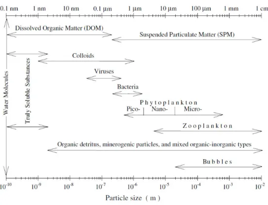
Figure 1.1. Size spectrum of seawater constituents between 0.1 nm and 1cm. Arrow ends indicate approximate boundaries for different constituent categories (source: Stramski et al. 2004). ... 6 Figure 1.2. Scanning Electron Microscopy images of particles retained on a GF/F glass fiber filter for a sample collected in the southern North Sea in September 2011, showing the enormous diversity in particle shapes and sizes. (A) Large diatom chains (microphytoplankton), large diatoms, and mineral particles. (B, C, D) Smaller particles: nanophytoplankton, and small minerogenic particles. (C) diatoms attached to a mineral particle. (D) coccolithophores. ... 7 Figure 1.3. Schematical geometrical configurations used to define absorption, scattering, and attenuation coefficients. (A) Fluxes of light when passing through a volume of seawater (after Morel 2008), (B) The elementary volume of thickness dx, seen as a point source from which originates the scattered radiation in all directions (after Morel 2008 and Mobley 1994) ... 9 Figure 1.4. (top) Spectral absorption and backscattering coefficients of pure seawater, phytoplankton, non-algal particles, and DOM (denoted by ‘w’, ‘ph’, ‘NAP’ and ‘CDOM’, respectively). Pure water absorption and scattering after Morel 1974; Pope and Fry 1997, respectively. (bottom) the resulting remote sensing reflectance computed from Eq. (1.21). ... 11 Figure 1.5. Geometrical configuration used for defining radiance (A), plane irradiance (B), and the coefficient for downwelling irradiance, Kd(B) (source: Morel 2008). ... 13

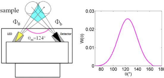
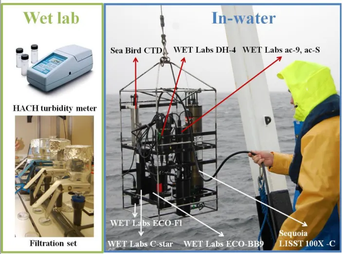
Figure 1.6. Typical transmissometer design (source: Pegau et al. 2003). ... 17 Figure 1.7. Source: Boss et al. 2009b (instruments compared in his paper are the WET Labs C-Star, WET Labs ac-9, LISST 100-B, and LISST-100X-FLOC) ... 18 Figure 1.8. Schematic of a volume scattering measurement for the WET Labs ECO BB-9 instrument and its angular weighting function (centroid anglem=124°). ... 20

Figure 1.9. (left) Frame with three Trios-RAMSES hyperspectral radiometers, installed on the prow of a research vessel. (right) Details of measurement configuration. ... 23 Figure 2.1. Procedural flow for the measurement of [SPM] of seawater. ... 27 Figure 2.2. Difference in filter weight before and after filtration of 250 mL of SSW of 34 PSU, with and without rinsing of the filter rim (step 13 in protocol in Figure 2.1). Grey dashed lines represent uncertainty on due to the detection limit of the balance, 0.14 mg. ... 33 Figure 2.3. Difference in filter weight before and after filtration vs. filtered volume of SSW of 34 PSU. Number of observations for each volume are 2, 6, 15, 95, 5, and 3, respectively. ... 33

Figure 2.4. Difference in filter weight before and after filtration, WD= , for different blanks collected at the start and the end of each campaign between 2007 and 2010. Grey dashed lines represent uncertainties on WD due to the detection limit of the balance ( 0.14 mg). ... 35 Figure 2.5. (a) Comparison of T before and after filtration, with statistics given using hand mixing and tumble mixing for all observations and in clear waters (Tb<5 FNU) and (b) relationship between T

and [SPM] with type II regression and statistics using hand mixing and tumble mixing. The 90% prediction bounds of the regression are also shown. Errorbars in (a) and (b) represent the standard deviation from replicate measurements of T and [SPM]. ... 36 Figure 2.6. Mixing methods for subsampling of seawater for filtration: (a) seawater is stirred up with a measuring cylinder and then subsampled using a 1L container, (b) seawater is mixed by gently tumbling a closed 10 L container mounted on a rotating frame attached to the wall in the wet lab of the ship. ... 36 Figure 2.7. Coefficient of variation, c.v. (in %) of [SPM], obtained from five replicates vs. filtration

volume, normalized to the optimal filtration volume, Vopt. Shown in grey are the median, 10

th

, and 90th percentiles of c.v. obtained from 100 resamplings without replacement of 3 [SPM] replicates out of 5. ... 40 Figure 2.8. Scanning Electron Microscopy images of two selected zones on the GF/F filter rim of sample MOD with filtration volume Vopt (a,b) or 2xVopt (c, d), showing particles that got displaced onto the

filter rim during the rinsing of the rim. ... 41 Figure 2.9. Boxplot of [SPM] obtained through filtration of different volumes of sampled seawater at six different stations. ... 42 Figure 2.10. Scatterplots of particulate dry mass ( ,) vs. filtrate volume. The errorbars denote the standard error on particulate dry mass obtained from 5 replicates. The mean and standard error of [SPM] are also shown for each filtration volume. Shown in red are the regression line and its equation with 95% confidence intervals of the coefficient estimates. ... 43 Figure 3.1. Location of stations sampled during 14 campaigns between April 2008 and July 2010. Bathymetry is also shown (source: General Bathymetric Chart of the Oceans, GEBCO_08 30’ Grid, version 20100927, http://www.gebco.net) ... 50 Figure 3.2. Instruments used in the wet lab of the ship (turbidity meter and filtration set) and instruments used for in-water measurements of optical properties (optical profiling package). ... 52 Figure 3.3. (A) Scatter plot of particulate beam attenuation (cp) measured simultaneously with LISST and

C-Star instruments, coded according to particle size (DA). The 1:1 line (solid) and the rejection

threshold line (log10(cp(LISST))=log10(cp (C-Star)-0.1124, dotted) are shown. (B) Scatter plot of cp(LISST): cp(C-Star) vs. DA. The type-II regression line (see section 3.5.1.3 for details) is shown,

with its equation and statistics. Error bars corresponding to uncertainties above 100% are not shown for clarity. (C) Scatter plot of cp measured simultaneously by the C-Star and the ac-s or ac-9. The 1:1

line is also shown. On each panel, error bars denote uncertainty estimates as derived in the section 3.5.1.2. ... 60 Figure 3.4. Log-log scatter plots of cp(LISST), cp(C-Star), bs, and bbp vs. area concentration, [AC] (left

column) and mass concentration, [SPM] (right column) for 35 case 1 and 72 case 2 waters. Error bars denote uncertainty estimates as derived in section 3.5.1, shown only for 20 random observations for the sake of clarity... 63 Figure 3.5.

c

m_p(C-Star) versus D_A1 in case 1 and case 2 waters. ... 65 Figure 3.6. Scatter plots of mass-specific beam attenuation,

c

m_p

(

LISST

)

vs. (A) the scattering cross

section (inverse of the product of apparent density and diameter, (a DA)

-1

), (B) the inverse of particle diameter weighted by area, DA

-1

, and (C) hyperbolic slope of the PSD. Modeling results of Boss et al. 2009a are shown for solid spherical particles (black lines) and for aggregates (grey lines) with refractive indices of 1.05+0.0001i (solid) and 1.15+0.0001i (dashed). Scatter plots of mass-specific backscatter,

b

_bpm vs. (D) (a DA)

-1

, (E) DA

-1

, (F) [POC]:([POC]+[PIC]), and (G) backscattering efficiency, Qbbe(=bbp:[AC]). Scatter plots of Qbbe vs.a (H) and DA (I). Error bars on all panels

denote uncertainties as derived in section 3.5.1.2. Equations and statistics of the fitted lines can be found in Table 3.2 and Table 3.3. ... 67 Figure 3.7. Mean particle apparent density (a) vs. mean particle diameter weighted by area (DA). The

relationship is shown for all data (black circles), for case 1 (grey dots) and case 2 waters (black dots). Statistics and equations of the type-II regression lines (see section 3.5.1.3 for details) fitted to each dataset are also shown. Error bars denote uncertainty estimates as derived in section 3.5.1.2. ... 68 Figure 3.8. Scatter plots of (A) cp(LISST), (B) cp(C-Star), (C) bbp, and (D) bs vs. [SPM]. Robust

regression lines are shown in black, together with their 90% prediction bounds, equations and statistics. (A, B) For comparison, the 90% prediction bounds of the cp(676 nm)-[SPM] data of Babin

et al. 2003 and the cp(650 nm)-[SPM] data of McKee and Cunningham 2006. ... 74

Figure 3.9. Scatter plots of the backscattering ratio, (=bbp:cp(LISST)) vs. (A) [POC]:([POC]+[PIC]), (B) [POM]:[SPM], (C) mean apparent density (a), and (D) [POC]:[SPM]. Regression lines, with

equations and statistics are shown on each panel (see section3.5.1 for details). Case 1 waters are shown in grey and case 2 waters in black. Error bars denote uncertainty estimates as derived in section 3.5.1.2. ... 77

Figure 3.10. Correlation coefficients of various scattering properties vs. area concentration, [AC]i, per

LISST size class in log log space for case 1 (A) and case 2 waters (C). Correlation coefficients of various scattering properties vs. the cumulative [AC]i , , in log log space for case 1(B)

and case 2 waters (D). Correlation coefficients between [AC]9(Di = 7.8m) and all other [AC]i in

log log space with 95% confidence intervals are shown in grey. ... 86 Figure 3.11. Correlation coefficients between area concentration recorded in each LISST size bin in case 1 (left) and case 2 (right) waters. ... 87 Figure 3.12. Coefficient of variation of cp(LISST) and bbp as function of mean particle size, DA. ... 89

Figure 3.13. Particle size distributions derived from a LISST-C instrument for 105 case 1 waters and 149 case 2 waters by particle number concentration (A), particle area concentration (B), and particle volume concentration (C). For clarity the median, 5th, and 95th percentile values are shown by the solid and dashed lines, respectively. (D) Median, 5th, and 95th percentile values of the normalized bias from the Junge power law model (see Eq. (3.4)) calculated as . ... 91 Figure 3.14. (A) Junge PSD slope vs. spectral slope of cp according to particulate absorption at 650 nm.

Jungian and non-Jungian PSDs are indicated by the black and red circles. Error bars denote standard errors on the retrieved slopes. The PSD slope models of Boss et al. 2001 and Morel 1973 are also shown, with model boundary represented by the dotted line. (B) Particle number PSDs normalized at 11 m and (C) spectra of cp normalized at 600 nm. ... 93

Figure 3.15. (A) Particle number PSDs normalized at 11 m for observations with cp spectral slope <0

and (B) normalized bias from the Junge PSD model. ... 94 Figure 4.1. Spatial extent of SEVIRI full disk imagery and viewing angle in degrees of SEVIRI on the MSG2-Meteosat9 platform located at 0°W (image kindly provided by Nicholas Clerbaux). ... 98 Figure 4.2. Normalized spectral response, (), of the SEVIRI solar channels (source: Govaerts and Clerici 2004) and one-way atmospheric transmittances for water vapor, ozone and molecular scattering for a vertical atmospheric path and the US standard atmosphere model simulated with LOWTRAN. ... 99 Figure 4.3. (A) SEVIRI Meteosat-9 full disk VIS06 image, (B) SEVIRI Meteosat-8 Rapid Scan Service (RSS) image. ... 100 Figure 4.4. Viewing angle of SEVIRI (on MSG2-Meteosat9 platform located at 0°W) over

Western-Europe. The white box delimits the study area, for which the northern limit corresponds to a 64° satellite viewing angle. The white dots are the locations for which daily variability of airmass and Rayleigh scattering are presented in Figure 4.5. ... 101

Figure 4.5. Variability of Rayleigh reflectance in the VIS06 band (grey lines) and total airmass (black lines) on (A) 15th June 2008 and (B) 15th December 2008 for the middle (dashed lines) and at the top (solid lines) of the SEVIRI subscene in Figure 4.4. ... 102 Figure 4.6. Normalized spectral response, () of SEVIRI’s VIS06, VIS08, and HRV bands, and

one-way total (

T

₀ ) and Rayleigh transmittance,

t

₀r, for a vertical atmospheric path and the US standard atmosphere model obtained from LOWTRAN simulations. Spectrum of solar irradiance at TOA from Thuillier et al. 2003. Thin lines represent above-water marine reflectance spectra,



_w0

(



)

, recorded with above-water TriOS Ramses radiometers in the southern North Sea between 2001 and 2010. The reader is referred to Ruddick et al. 2006 for details on the seaborne measurement protocol. ... 105 Figure 4.7. Marine reflectances in the VIS06 and VIS08 bands obtained from optimal in situ above-water marine reflectance measurements collected between 2001 and 2010 in the southern North Sea waters. The parameter



is calibrated through linear regression (black line) of 47 reflectance measurements for which



_w0(0.8)<0.011. ... 111 Figure 4.8. Identification of clear water pixels from which the VIS06:VIS08 band ratio of aerosol reflectance,, is obtained. The black rectangles delineate the clear water pixels identified by Neukermans et al. 2009, while the red polygons delineate the revised clear water pixels. Background: SPM (in mg L-1) map from SEVIRI on February 11, 2008 at 10:45 UTC. The location of the Cefas SmartBuoys at Warp Anchorage (TH1), West Gabbard (WG), and Dowsing (D), used in Chapter 5 is also indicated. ... 112 Figure 4.9. Example of the estimation of the VIS06:VIS08 band ratio of aerosol reflectances, , on April 9, 2008 at 09:45 UTC from the Rayleigh and gas corrected reflectances,



_c, in the VIS06 and VIS08 bands of clear water pixels via (a) the mean and standard error of



_c(0.6):



_c(0.8)values, shown as the normal fit to the histogram, or (b) via linear regression of



_c(0.6) vs.



_c(0.8), with uncertainties on regression coefficients given by their standard error. N is the number of pixels.... 113 Figure 4.10. Schematical depiction of the processing steps in the atmospheric correction of the SEVIRI VIS06 and VIS08 channels. The second pass in the two-pass algorithm is represented by the blue lines (in the first pass, shown by the orange lines,





1

). ... 115 Figure 4.11. (a) Linear regression of above-water marine reflectance in the HRV and the VIS06 bands and (b) linear regression of marine reflectance of the HRV band at TOA, normalized by two-way

atmospheric transmittance in the VIS06 band vs. above-water marine reflectance in the VIS06 band. ... 116 Figure 4.12. Normalized spectral response of the SEVIRI meteorological satellite (black) and the MODIS-Aqua ocean colour satellite (grey). ... 123 Figure 4.13. Marine reflectances in the SEVIRI VIS06 band and the MODIS Aqua 645 nm band obtained from optimal in situ above-water marine reflectance measurements collected between 2001 and 2010 in the southern North Sea waters. The least-squares linear regression through the origin is shown with equation and 95% confidence interval on the slope estimate. ... 123 Figure 4.14. (A) Marine reflectance from SEVIRI VIS06 on 16-02-08 at 13:00 h UTC and (B) associated relative uncertainty in %, obtained from Eq. (4.51). ... 124 Figure 4.15. Uncertainty components of SEVIRI VIS06 marine reflectance on 16-02-2008 at 13:00 h UTC. (A) total uncertainty as in Eq. (4.51), (B) digitization uncertainty as in Eq. (4.50), (C) uncertainty due to aerosol turbidity as in the first term of Eq. (4.47), and (D) uncertainty due to water turbidity as in the second term of Eq. (4.47). ... 125 Figure 4.16. Marine reflectance on 16-02-2008 at 13:00 h UTC for a subset of the SEVIRI southern North Sea scene on (A) the SEVIRI VIS06 grid with a spatial resolution of 3 km x 6.5 km and (B) on the HRV grid with a spatial resolution of 1 km x 2 km. Circles represent five selected stations for which diurnal variability of marine reflectances is shown in Figure 4.20. ... 126 Figure 4.17. Maps of marine reflectances from the SEVIRI VIS06 band (left) and MODIS Aqua 645nm band (right), acquired on (from top to bottom): 11 Feb. 2008 at 12:45 h UTC, 6 May 2008 at 13:00 h UTC, 23 July 2008 at 13:15 h UTC, and on 8 March 2009 at 13:00 h UTC. Corresponding scatter plots are shown in Figure 4.18. ... 127 Figure 4.18. Scatter plots of SEVIRI VIS06 marine reflectance vs. MODIS Aqua 645nm reflectances, acquired on (A) 11 Feb. 2008 at 12:45 h UTC, (B) 6 May 2008 at 13:00 h UTC, (C) 23 July 2008 at 13:15 h UTC, and on (D) 8 March 2009 at 13:00 h UTC, corresponding to the scenes shown in Figure 4.17. The least-squares regression and statistics are shown, as well as the 1:1 line (dashed). ... 128 Figure 4.19. Trends in SEVIRI-MODIS reflectance match-ups statistics. Scatter plots of (A) median VIS06 reflectance vs. the 95th percentile value of the normalized absolute error, NAE and (B) the 5th percentile of VIS06 reflectance vs. the median normalized bias, NB. ... 130 Figure 4.20. Diurnal variability of SEVIRI VIS06 marine reflectance (left) and the VIS06:VIS08 band ratio of aerosol reflectance (right) on three cloud free days: 11 February 2008 (top), 8 April 2008 (middle), and 1 April 2009 (bottom). Time series of marine reflectance are plotted at P1 (blue), P2 (green), P3 (red), P4 (cyan), and P5 (purple), with location shown in Figure 4.16. Errorbars denote

uncertainties on marine reflectance derived from Eq. (4.51) or on  from the standard error of slope estimate. ... 133 Figure 4.21. Effect of the atmospheric correction assumption (4.22) on the retrieval of



_w0(0.6): normalized bias of



_w0(0.6) obtained from Eq. (4.34) from the true marine reflectance for





0

.

84

(diamonds),





1

.

02

(circles), and





1

.

30

(crosses), with simplifications





1



t

_oa_,(_v0.8). The dashed line corresponds to the reflectance region where  was calibrated (see Figure 4.7). ... 135 Figure 4.22. MODIS 2009 climatology of marine reflectance at 645 nm. The yellow polygon delineates the SEVIRI full disk coverage and the red polygons indicate waters that are sufficiently turbid to be reliably detected by SEVIRI. ... 138 Figure 4.23. Estimation of VIS06:NIR16 ratio of aerosol reflectances. (a) Rayleigh corrected reflectances for a set of clear water pixels in VIS06 and NIR16 bands on June 29th 2006 at 11:30UTC. (b) The corresponding histogram of the VIS06:NIR16 Rayleigh corrected reflectance ratios (N is the number of pixels). ... 140 Figure 4.24. Estimation of VIS06:VIS08 ratio of aerosol reflectances. (a) Rayleigh corrected reflectances for a set of clear water pixels in VIS06 and VIS08 bands on June 29th 2006 at 11:30UTC. (b) The corresponding histogram of the VIS06:VIS08 Rayleigh corrected reflectance ratios (N is the number of pixels). ... 140 Figure 4.25. Effectiveness of SEVIRI VIS06-VIS08 inter-calibration method using the offset of the regression of their Rayleigh and gas corrected reflectances,



_c(0.6)and



_c(0.8). Variation of ,



_a(0.8), and



_w0(0.6)with uncertainty



A

₀(0.8)on the VIS08 calibration factor (A) or with uncertainty



A

₀(0.6) on the VIS06 calibration factor (B). (C) Scatter plot of



_c(0.6)vs.



_c(0.8) for



A

₀(0.8)= -0.05 (black dots) and



A

₀(0.8)= 0.05 (grey circles) with fitted regression lines. (D) same as (C) but for



A

₀(0.6)= -0.05 and



A

₀(0.6)= 0.05. (data for 8 April 2008 at 12:00UTC were used). ... 144 Figure 5.1. Scatterplot of 68 seaborne measurements of marine reflectance in the VIS06 band, and turbidity (T) and SPM concentration (S). The black and grey lines represent the SEVIRI VIS06 retrieval algorithms for T (Nechad et al. 2009) and S (Nechad et al. 2009; Nechad et al. 2010) with C=0.1639. The RMSE and the [5 50 95]th percentiles of the relative model prediction errors are also shown. ... 148 Figure 5.2. Scatter plots of SEVIRI vs. SmartBuoy turbidity (T) and light attenuation (KPAR) at TH1, WG,

Regression and 1:1 lines are shown in red and black, respectively, with equations and statistics in Table 3. Quality flagged observations are shown in grey and correspond to pixels where either the SEVIRI marine reflectances have over 100% uncertainty (a,b,c,d), or are in the proximity of cloud or low aerosol transmittance pixels (c, d), or low quality PAR measurements (c, d). Errorbars are plotted for 1% random observations and denote uncertainties on SmartBuoy (Eq. (5.7)) and SEVIRI (Eqs. (5.2) and (5.5)) products. Regression outliers are labelled by white crosses. ... 153 Figure 5.3. Randomly selected original and smoothed time series of T obtained from SEVIRI and SmartBuoys. SEVIRI T data from the VIS06 and HRV bands with uncertainty from Eq. (5.2) are shown by the black and grey errorbars, respectively. Temporally smoothed data series for VIS06 and HRV T products are shown by grey circles and diamonds, respectively, with global (big red dot) and local (small red dots) maxima. SmartBuoy T and its uncertainty is shown by the blue errorbars, while the temporally smoothed data series is shown by blue circles with local maxima highlighted in cyan. Grey vertical dotted lines represent data availability from MODIS Aqua. ... 156 Figure 5.4. Continuation of Figure 5.3. ... 157 Figure 5.5. Scatterplot of the timing of maximum turbidity derived from the SmartBuoys (TH1, WG, and D) and SEVIRI on 49 cloudfree periods. The 1:1 line (solid) and 1 hour offset lines (dashed) are shown in black. Labels refer to the time series shown in Figure 5.3 and Figure 5.4. The mean and standard deviation of the phase difference, median and 5th-95th percentile interval for prediction error and bias are also given in black. ... 158 Figure 5.6. Six randomly selected original and smoothed time series of Kdobtained from SEVIRI and

SmartBuoys. SEVIRI KPAR data from the VIS06 and HRV bands with uncertainty expressed by

Eq.(5.5) are shown by the dark and light grey errorbars, respectively. Temporally smoothed data series for VIS06 and HRV KPAR products are shown by grey circles and diamonds, respectively, with

global (big red dot) and local (small red dots) maxima. SmartBuoy KPAR and uncertainty (after Eq.

(5.7)) are shown by the blue errorbars, while the temporally smoothed data series are shown by blue circles with local maxima highlighted in cyan. Grey vertical dotted lines represent data availability from MODIS Aqua. The yellow crosses indicate quality flagged KPAR SmartBuoy data (from Eq.

(5.8)). ... 159 Figure 5.7. Scatterplot of the timing of maximum PAR attenuation derived from the SmartBuoys (TH1 and D) and SEVIRI during 27 cloudfree periods. The 1:1 line (solid) and 1 hour offset lines (dashed) are shown in black. Labels refer to the time series shown in Figure 5.6. The mean and standard deviation of the phase difference, median and 5th-95th percentile interval for prediction error and bias are also given in black. ... 160

Figure 5.8. Effect of the atmospheric correction assumption of constant , as in Eq. (4.22), on the retrieval of T from



_w0(0.6): normalized bias of T retrieved by SEVIRI (after Eq. (4.34)) from the true T (=T algorithm applied to the in situ marine reflectance) for





0

.

84

(diamonds),





1

.

02

(circles), and





1

.

30

(crosses), with simplifications





1



t

_oa_,(_v0.8). The dashed line demarcates the reflectance region where  was calibrated (see Figure 4.7). ... 162 Figure 5.9. Investigation of SEVIRI VIS06 sub-pixel scale variability using MODIS Aqua imagery. (A) Scatter plot of 5 x 5 km² spatial mean turbidity from MODIS 645nm at WG and TH1 for the period 2002-2010 vs. the 1 x 1 km² center pixel turbidity, (B) Scatter plot of MODIS 645nm turbidity vs. SmartBuoy turbidity (TSB) at TH1 and WG. (C) same as (B) but using the 5 x 5 km² spatial mean value. Regression and 1:1 lines are shown in red and black respectively. Regression outliers are marked by white crosses. The turbidity algorithm of Nechad et al. 2009 was used. ... 163 Figure 5.10. Scatter plot and regression analysis of the particulate backscattering coefficient vs. simulated SmartBuoy turbidity (scattering between 15° and 150°) obtained from in-situ measurements with the WET Labs MASCOT instrument (=658 nm, Sullivan and Twardowski 2009) collected in a wide diversity of coastal and offshore waters. ... 166 Figure 5.11. Relationship between [SPM] and turbidity recorded before filtration (Tb) for the hand mix

and tumble mix dataset. Black lines denote the 90% prediction bounds of the [SPM] vs. Tb

relationship for the tumble mix dataset, outside which data were rejected. The regression line equations and statistics are also shown, with n0 denoting the number of observations and R² the

coefficient of determination. ... 170 Figure 5.12. SEVIRI VIS06 single band [SPM] retrieval algorithm calibrated with datasets collected in the southern North Sea during the periods 2001-2006 and 2007-2010. ... 171 Figure 5.13. (a) Relationship between the particulate backscattering coefficient, bbp (=650nm), and

turbidity in clear (case 1) and turbid (case 2) waters. The regression line with its 90% confidence bounds in log-log scale and statistics are shown (MPE= median PE). (b) Variability of T-specific bbp

as a function of particle composition. The fitted regression and statistics can be found in. See also Chapter 3 for details on in situ measurement and data treatment. ... 172 Figure 5.14. Influence of the variability of the mass-specific backscattering coefficient, , on the suspended matter retrieval algorithm of Nechad et al. 2010 for the SEVIRI VIS06 band, calibrated with southern North Sea (SNS) in-situ data (solid black line). (left) Dashed lines represent the [SPM] algorithm corresponding to a factor 4 variability in As. Error bars indicate measurement

uncertainties. French Guyana (FG) data are also shown. (right) relationship between and the normalized bias of the [SPM] algorithm for SNS (grey dots) and FG data (black squares). ... 175

Figure 5.15. Some selected time series of T from SEVIRI on the VIS06 grid and modelled bottom stress at P2 (see Figure 4.16 for location). Global maxima are indicated by the large red dots, small dots indicate local maxima (red) and minima (green). Errorbars denote uncertainties on T after Eq. (5.2). ... 177 Figure 5.16. Scatterplot of the timing of maximum T from SEVIRI vs. timing of maximum bottom stress during cloudfree periods at P1 (A) and P2 (B) with location given in Figure 4.16. The 1:1 line (solid) and 1 hour offset lines (dashed) are shown in black. The observed mean and standard deviation of the phase difference, median and 5th-95th percentile interval for bias are shown in black. The red numbers refer to the same statistics obtained for a random timing of maximum bottom stress. ... 177 Figure 6.1. Diurnal variability of remote sensing reflectance (Rrs) in the VIS and NIR as recorded by

GOCI on 13 June 2011 at a station in the Bohai Sea (source: Ruddick et al. submitted). SEVIRI’s red band approximate spectral coverage is also shown. ... 181 Figure 6.2. MODIS 2009 climatology of marine reflectance at 645 nm. Spatial coverage of

MSG-SEVIRI, Electro-MSU, and COMS-GOCI are shown by the yellow, orange, and green polygons, respectively. Red polygons indicate waters that are expected to be detectable by MSU. ... 183

L

IST OF

T

ABLES

Table 2.1. Overview of types of [SPM] procedural control filters and treatments. ... 28 Table 2.2. Overview of water samples collected in the southern North Sea for filtration experiments with salinity, temperature, chlorophyll a concentration, and turbidity, T , with standard deviation T. .... 31 Table 2.3. Lookup table for recommended filtration volume as function of turbidity so that relative uncertainty on [SPM] replicates is within 15% in 50% of the cases (R(V50)) and in 90% of the cases

(R(V90)). ... 38

Table 2.4. Overview of turbidity, T , with standard deviation T, optimal filtration volume obtained from R(V90) in Table 2.3, and time required to pass seawater through five replicate filters. ... 39

Table 3.1. Correlation coefficients (r with 95% confidence interval, see section 3.5.1.4 for computation) between an optical property and either area concentration, [AC], or mass concentration, [SPM] (in log log space) for 107 observations (35 case 1 and 72 case 2). The median, 5th, and 95th percentile values of mass- and area-specific optical properties are shown. Correlations and mass-specific coefficients for all simultaneous observations of an optical property and [SPM] are also shown between brackets (database size, nt, is indicated in italic). ... 62

Table 3.2. Correlations and regression analysis of mass-specific attenuation (

c

m_p) and backscattering (

m bp

b

) vs. mean particle diameter (DA), mean apparent density (a), mean optical efficiency factors

(Qce, Qbbe), and particle composition. ns: not significant (i.e., p>0.05), *: p<0.001, no is the number of

observations, nx is the number of outliers removed as described in section 3.5.1.3... 66

Table 3.3. Correlations and regression analysis of optical efficiency factors (Qce, Qbbe) vs. mean particle

diameter (DA), mean apparent density (a), and particle composition. ns: not significant (i.e., p>0.05),

*: p<0.001, no is the number of observations, nx is the number of outliers removed as described in

section 3.5.1.3. ... 72 Table 3.4. Optical properties as proxies for [SPM]. Prediction percentile error, PPE, i.e., the ratio of the absolute value of the difference between a type-II regression model derived [SPM] and its observed value to its observed value. Values between brackets for an optical model with 1.2<[SPM]<82.4 g m-3 for our dataset and for the dataset of Boss et al. 2009c in italic. r is the correlation coefficient with its 95% confidence interval (see section 3.5.1.4 for details). ... 75 Table 3.5. Uncertainty estimates on optical and particle concentration measurements, and their derived quantities. ... 81