On the Efficiency of the Linear-mode Conversion for Generation of Solar Type III Radio Bursts

HAL Id: insu-02519403

https://hal-insu.archives-ouvertes.fr/insu-02519403

Submitted on 26 Mar 2020

HAL is a multi-disciplinary open access

archive for the deposit and dissemination of

sci-entific research documents, whether they are

pub-lished or not. The documents may come from

teaching and research institutions in France or

abroad, or from public or private research centers.

L’archive ouverte pluridisciplinaire HAL, est

destinée au dépôt et à la diffusion de documents

scientifiques de niveau recherche, publiés ou non,

émanant des établissements d’enseignement et de

recherche français ou étrangers, des laboratoires

publics ou privés.

On the Efficiency of the Linear-mode Conversion for

Generation of Solar Type III Radio Bursts

Vladimir Krasnoselskikh, Andrii Voshchepynets, Milan Maksimovic

To cite this version:

Vladimir Krasnoselskikh, Andrii Voshchepynets, Milan Maksimovic. On the Efficiency of the

Linear-mode Conversion for Generation of Solar Type III Radio Bursts. The Astrophysical Journal, American

Astronomical Society, 2019, 879 (1), pp.51. �10.3847/1538-4357/ab22bf�. �insu-02519403�

On the Ef

ficiency of the Linear-mode Conversion for Generation of Solar Type III Radio

Bursts

Vladimir Krasnoselskikh1 , Andrii Voshchepynets2 , and Milan Maksimovic3

1

LPC2E/CNRS, UMR 7328, 3A Avenue de la Recherche Scientifique, Orleans, France;vkrasnos@cnrs-orleans.fr

2

The Swedish Institute of Space Physics(IRF), Rymdcampus 1, Kiruna, Sweden 3_{LESIA/CNRS, Paris Observatory, Paris, France}

Received 2019 January 30; revised 2019 April 25; accepted 2019 April 30; published 2019 July 3

Abstract

Type III solar radio bursts are generated by streams of energetic electrons accelerated at the Sun during periods of solar activity. The generation occurs in two steps. Initially, electron beams generate electrostatic Langmuir waves and then these waves are transformed into electromagnetic emissions. Recent studies showed that the level of densityfluctuations in the solar wind and in the solar corona is so high that it may significantly affect beam–plasma interaction. Here, we show that the presence of intense densityfluctuations not only crucially influences the process of beam–plasma interaction, but also changes the mechanism of energy transfer from electrostatic waves into electromagnetic. Reflection of the Langmuir waves from the density inhomogeneities may result in partial transformation of the energy of electrostatic waves into electromagnetic around plasma frequency. We show that the linear wave energy transformation for the level offluctuations of the order of 1% or higher is efficient enough to produce radio bursts with a brightness temperature of 1014–1015K.

Key words: acceleration of particles – solar wind – Sun: particle emission – Sun: radio radiation 1. Introduction

Solar type III radio bursts are among the strongest radio emissions in the heliosphere. It is widely accepted that the high energy electrons ∼5–30 keV, accelerated during reconnection of the magneticflied lines in solar atmosphere, are responsible for the generation of this radio emission(Suzuki & Dulk1985; Melrose2017). An important characteristic of the type III radio

bursts is the fast frequency drift rate(Wild & McCready1950).

Type III bursts can start at a frequency of several hundreds of MHz and then go down to tens of kHz within a few minutes with the increasing duration at a given frequency (Alvarez 1973; Krupar et al. 2018; Reid & Kontar 2018). To

explain the frequency drift, the beams should have near relativistic speeds 0.1–0.5c (Melrose1990), and generate radio

emission near local plasma frequency, fpe, and double plasma

frequency (harmonic; Ginzburg & Zhelezniakov 1958).

Fre-quency of the emission varies with local electron density along the beam path, it starts at the high frequencies in dense plasma close to the Sun and then decreases over time as the beam propagates in the expanding solar corona and later in solar wind(Krupar et al. 2018).

Generation of radio waves occurs in two steps. In the original study, Ginzburg & Zhelezniakov(1958) proposed that

the two-stream instability of an electron beam results in the growth of electrostatic(ES) Langmuir waves that later produce electromagnetic(EM) emission at the plasma frequency due to the induced scattering on ions, while the coalescence of two Langmuir waves can produce the harmonic emission. The theory has been subsequently refined and alternative mechan-isms for the conversion of the beam-driven Langmuir waves into EM radiation have been proposed (Melrose 1990; Malaspina et al. 2012; Volokitin & Krafft 2018). While the

exact mechanism of the ES to EM conversion is still under debate, the generation of the Langmuir waves by electron beams in the solar wind has been confirmed by in situ measurements (Lin et al.1981; Ergun et al.1998).

Beam-type configurations in a plasma are known to be unstable, and relaxation of the beam–plasma system to the stable state results in growth of the Langmuir turbulence (Romanov & Filippov1961; Drummond & Rosenbluth 1962; Vedenov 1963). Landau resonance enables effective energy

transfer from the beam electrons to the waves, and as a result, up to two-thirds of the initial beam energy can be transferred to the Langmuir waves through wave–particle interaction (Vede-nov & Ryutov1975). Recent studies have shown that the level

of densityfluctuations in the solar wind and in the solar corona are so high that they may significantly affect beam–plasma interaction (Kontar 2001; Zaslavsky et al. 2010; Krafft et al.

2013; Reid & Kontar2013; Voshchepynets et al.2015). The

presence of the densityfluctuations causes changes in the phase velocity of the Langmuir waves, and as a result affects resonant velocities of the electrons. This leads to a significant decrease of the increment of instability and an important increase of the relaxation length of the beam (Voshchepynets & Krasnoselskikh2015).

The presence of the density fluctuations has a significant impact on the observed properties of the Langmuir waves(see Krasnoselskikh et al. 2007 and references therein). First, this idea has been proposed in Smith & Sime (1979) in order to

explain observed clumping of Langmuir waves in type III source regions. Later, it has been shown (Ergun et al. 2008)

that the density irregularities in the solar wind can form cavities and can cause modulation of the the waveforms of the Langmuir waves. Analysis of the large number of individual waveforms measured by STEREO and WIND showed good agreement with theoretical predictions (Ergun et al. 2008; Malaspina & Ergun 2008) and results of the numerical

simulations(Krafft et al.2014). Several statistical models have

been proposed to take into account the influence of random density fluctuations on generation and statistics of Langmuir waves. Thefirst was the stochastic growth theory by Robinson et al.(1993). It predicted that the distribution of the amplitudes

of the Langmuir waves in type III source regions should

correspond to log-normal distribution. While some observa-tions (Robinson et al. 1993; Píša et al. 2015) show good

agreement with this prediction, there are numerous reports of observations and simulations (Krasnoselskikh et al. 2007; Vidojevic et al. 2012; Reid & Kontar 2017; Voshchepynets et al. 2017) that show deviations of the distribution of the

amplitudes of the Langmuir waves from log-normal can be rather significant.

The aim of the present study is to determine the role of the density fluctuation in the conversion process of the beam-generated ES waves into EM emissions around plasma frequency. Reflection of the Langmuir waves from the density inhomogeneities may result in partial transformation of the energy of ES waves into EM. We consider this effect of linear wave energy transformation in application to the generation of type III solar radio bursts. We use the probability distribution of densityfluctuations to evaluate the statistical characteristics of such a process and its efficiency. We show that the mechanism of linear transformation for the relative density fluctuations of the order of 1% is efficient for producing radio emission with a brightness temperature of 1014–1015K(Suzuki & Dulk1985; Saint-Hilaire et al.2013). The influence of wave

reflection on random density fluctuations on the generation of harmonic emission will be studied in a forthcoming paper.

2. Calculation of the Efficiency of Energy Conversion When the density fluctuations along the waves path cannot be neglected, the propagation of the wave can be described with a nonlinear Bohm–Gross dispersion relation for Langmuir waves ⎛ ⎝ ⎜ ⎞_⎠⎟ ( ) w =w + l k + dn N 1 3 , 1 p D 2 2 2 2 0

where ω and k are the frequency and wave vector of the Langmuir wave, wp is the electron plasma frequency for the

electron number density N0, dn is a deviation of the density

from the average value N0, and lD is the Debye length. The

waves are assumed to be generated resonantly, w = kVb, where

Vb is the beam velocity that significantly exceeds thermal

velocity of electrons vT = T m (T and m are electron

temperature and mass, respectively). A Langmuir wave propagating in plasma with density inhomogeneities encounters density depletions and enhancements along its path. The characteristic scale of density inhomogeneities is supposed to be much larger than the wavelength of Langmuir waves. When the wave goes to the increasing density region where the wave frequencyω approaches the local plasma frequency wp(a more

precise condition will be presented below), the wave is reflected.

Assuming that the density fluctuations are isotropic, the incident angles of Langmuir waves are distributed uniformly over a semisphere. For the majority of incidence angles, the reflection resembles a mirror-type reflection; the k-vector component parallel to the direction of the density gradient changes its direction, while the k-vector component perpend-icular to the gradient remains unchanged. In the rather narrow range of incidence angles, ES waves may couple with the EM and the process becomes a three-wave coupling process. In this case, the reflection results in a Langmuir wave and an EM wave, so that a part of the incident Langmuir wave energy is

transformed to the EM wave. It is worth noting that initial reflection generates an EM wave propagating in the direction opposite to the incident direction of the ES wave, i.e., initial EM emission will be generated toward the Sun, if applied to the solar type III radio burst. However, as an average density decreases with the distance from the Sun, the secondary reflections that may be considered as mirror type, will turn the wave direction toward the Earth(top panel in Figure1).

Following the previous works (Piliya 1966; Stenzel et al.

1974), the Langmuir wave of frequency ω propagates obliquely

to the direction of the density gradient that we choose to be along the z-axis (panel (c) in Figure1). The majority of studies

on this topic are dedicated to the transformation of an EM wave into ES in the vicinity of the reflection point. This problem is conventionally called a “direct” problem; the problem we address here is“inverse,” the transformation of ES waves onto EM. As it was shown by Hinkel-Lipsker et al. (1989) the

reflection coefficient for the both problems are equal in magnitude and the corresponding mode-conversion coefficients satisfy energy conservation. We let the perpendicular comp-onent of the k-vector be directed along the x-axis and be equal tokx=k sinY, whereΨ is the incidence angle of ES wave. So

the k component along the z-axis is

( ) ( ) w w = - -k T m k 3 . 2 z p x 2 2 2

When the density profile is a linear function of distance with characteristic scale L, that is supposed to satisfy the condition

)  w L c , one finds ⎜ ⎟ ⎛ ⎝ ⎞⎠ ( ) ( ) ( ) d w w + _{= = +} N n z N z z L 1 , 3 p p 0 0 2 0 2

so the incident Langmuir wave reflects when the local plasma frequency is ( ) ( ) w z =w - T Y mV 1 3 sin . 4 p b2 2

A fraction of incident wave energy is reflected as a Langmuir wave, while the other part is converted to an EM wave in this mode-conversion point wp( )z =w. The EM wave propagates

outward into the direction of the density decrease beyond its cutoff frequency atwp( )z =wcosq, where angleθ corresponds to the angle of propagation of the EM wave with respect to the z-direction. Here we consider the mirror type; the kxcomponent

remains unchanged and it is the same for the incident ES wave and reflected ES and EM waves. As such, a relation between Ψ andθ could be found assinY = V c( b )sinq.

The problem has been studied by many authors starting with the pioneering work by Denisov(1957). Several methods have

been developed to evaluate the conversion coefficient, (e.g., review by Piliya1966). Hinkel-Lipsker et al. (1989,1991) have

performed analytical study and obtained an analytical expres-sion for the converexpres-sion coefficient

∣ ∣ ∣ ∣ ( ) [ ( )] [ ( ( )) ] [( ( )] [ ( )] ( ) h p p p = -= ¢ + ¢ + ¢ ¢ R q Ai q q Ai q q Ai q Bi q 1 2 1 , 5 2 2 2 2 2 2 2 4 2 2 2

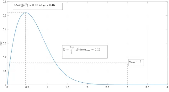
where R is the reflection coefficient defined as the ratio of the reflected Langmuir wave amplitude to the amplitude of the incident wave, η is the ratio of the EM and the incident Langmuir wave amplitudes,q =(wL c)2 3sin2q_{, Ai(q), and Bi} (q) are Airy functions, and Ai′(q) and Bi′(q) their derivatives. The dependence of the energy conversion coefficient on parameter q is shown in Figure2.

It is convenient to re-write the reflection coefficient in terms of the incidence angle of the Langmuir waveΨ. The parameter q can be written as ⎜ ⎟ ⎛ ⎝ ⎞⎠ ⎛ ⎝ ⎜ ⎞ ⎠ ⎟ ( ) w ( ) w Y = Y q L L c k c , sin , 6 2 3 2 2 2 2

Figure 1.Schematic illustration of the formation of the type III solar radio bursts.(a) Electron beam ejected from the Sun generates an ES (Langmuir) wave due to the bump-on-tail instability. Frequency of the ES wave is equal to the local plasma frequency of the solar wind. The wave propagates out from the Sun to the region with lower electron density(density profile of the solar wind is shown with a blue line). (b) Langmuir wave L undergoes reflection on the density fluctuation N1. The reflection results in the reflected Langmuir wave L′ and EM wave t:  ¢ +L L t. Both ¢L and t propagate toward the Sun until they undergo second reflection on the density gradient or another densityfluctuation N2:t ¢t . The reflected EM wave ¢t propagates away from the Sun and can be detected by a remote observer. (c) Detailed illustration of the ES–EM transformation. Local density gradient caused by density fluctuation is along the z-axis. The ES wave propagates obliquely with an angleΨ to the direction of the density gradient (z-axis). It undergoes reflection at the point where the component of the k-vector along the density gradient becomes equal to 0. The reflection results in a secondary ES wave and an EM wave. Angle q corresponds to the angle of propagation of the EM wave with respect to the z-axis.

where L is the characteristic density inhomogeneity scale. As one can see from Figure2, ∣ ∣h2 _{reaches its maximum of∼0.52} at q~0.46 and decreases rapidly with increasing q. For instance for q=2, the corresponding value of transformation coefficient is ∼0.01, while for q=6, ∣ ∣h ~2 2.5·10-12_{. Due} to such rapid decrease we consider a limited range of the q parameter:0<q<q_{max. For this study we choose q}maxto be

equal to 3, since for q>qmaxthe transformation coefficient is

very small (<2.5 · 10−4).

In our probabilistic model, the efficiency of the beam-generated Langmuir wave’s conversion into EM emission is evaluated by averaging over angles and the densityfluctuation scales. To evaluate the ensemble averaged values, taking into account the probability distribution of the densityfluctuations, we choose hereafter the reference frame, where the z-axis is directed along the wave vector of the propagating Langmuir wave. The average probability can be written as the product of probability distributions in angle PΨ(Ψ) and in scale PL(L)

( ) ( )∣ ( )∣ ( )

ò

h = = Y Y Y < < Y K W W P P P L L, d dL, 7 t L q q L eff ref 0 2 max

where Keff is the energy conversion coefficient from ES

Langmuir waves to EM, Wtis energy density of reflected EM

wave, WLis the energy density of incident Langmuir wave, and

Prefis the probability of ES wave reflection. As it was shown in

Voshchepynets et al. (2015) and Voshchepynets &

Krasno-selskikh (2015), in the plasma with random density

fluctua-tions, Pref can be calculated by making use of a probability

distribution function of the amplitudes of the density fluctua-tionsP n N(d 0).

Since the conversion occurs only when the parameter q is in the range from about 0 to qmax, this leads to the limited angular

range of reflected EM waves, given by

⎜ ⎟ ⎜ ⎟ ⎛ ⎝ ⎞⎠ ⎛ ⎝ ⎞ ⎠ ( ) w w < Y < q c L kc 0 sin _max1 2 . 8 1 3

Taking into account that the k-vector of the Langmuir wave is approximately equal tokL w Vb, the conversion may occur

only when the angleΨ is given by

⎜ ⎟ ⎛ ⎝w ⎞⎠ ( ) < Y < q V c c L 0 arcsin _max1 2 b . 9 1 3

To simplify the evaluation of the integrals, we shall take the conversion coefficient to be approximately constant, corresp-onding to its average value ∣ (h L,Y)∣2 =Q0.16_{in the range} of q between zero and qmax=3. Here it should be noted that Q

depends on qmax. For the lower q (0.2<q <3), the averaged

value Q is higher as only fluctuations that cause effective transformation (with ∣ ∣h >2 10-4_{) are considered. For} qmax>3, the averaged value is lower because the

transforma-tion coefficient is almost zero (Figure 2). Under this

assumption, the integration over angles and scales L may be carried out independently step by step. Assuming uniform distribution over angles, PY( )Y =( )p-1 _{and taking into} account that Ymaxqmax(c (wL)) (V cb )

1 2 1 3 _{, the integration}

over angles results in

⎜ ⎟ ⎛ ⎝ ⎞⎠ ( ) ( )

ò

Y PY Y Y =d _pq V _w c c L 1 . 10 b 0 max 1 2 1 3 max

Here we replace arcsinYmax by its argument, taking into account that both are small. Then, the conversion coefficient may be rewritten as ⎜ ⎟ ⎛ ⎝ ⎞⎠

ò

( ) ( ) p w = ¥ K Qq V c c L P L dL 2 1 , 11 b L eff max 1 2 _{1 3} 0 1 3

where PL(L) is the probability distribution of the density

gradients (scales). One should note that the low limit of integration should have been limited by some Lmin, where the spectrum of densityfluctuations sharply decreases or has a cut off. But as we shall see further, the probability distribution

( )

P LL decreases rapidly for small values of L, thus the limit

may be taken to be zero.

In order to calculate PL(L) one should use spatial profiles of

the densityfluctuations. In the present study we use synthetic density data calculated from published density power spectra. Kellogg et al. (1999) proposed a procedure based on the

inverse Fourier transform that allows us to reconstruct density profiles n(t) from the power spectrum, assuming the phases of waves to be random. It is known from in situ spacecraft measurements in the solar wind (Celnikier et al. 1987; Chen et al.2012) that the density spectrum can be considered as a

broken power law, with different spectral indices (about 5/3 for the low frequency part, and about 1 for the higher frequency part with the transition at about 0.6 Hz). In order to transform these profiles to the spatial profiles n(z), one can use the Taylor hypothesis, assuming thatfluctuations are convected with the characteristic velocity of the solar wind, VSW. We used a power

spectrum in the range of frequencies between 10−2Hz and 530 Hz. The lower frequency limit defines the maximal length of the synthetic density profiles (100 s or 4 ·10 km4 _for VSW∼400 km s−1). The highest frequency limit defines the

smallest scale of the density fluctuation presented in these profiles. In the present study this scale is set to be approximately 750 m and for the plasma conditions relevant for 1 au it is about50lD. After the profiles were generated,

normalization procedure was applied to ensure that ( )

án zñ =z N0 and á( ( )n z -N0)2ñ =z dn for each of the

density profiles (here brackets denote averaging). We consider different levels of density fluctuations, dn N0, between 0.01 and 0.1. For more details on the procedure we refer to Voshchepynets & Krasnoselskikh(2015).

Locally, the density profiles may be approximated by the linear function ofn z( ) and the probability distribution of the characteristic scales could be retrieved from the distribution of density gradients, (1 n) = ¶n lnn z( ) ¶z = 1 L. The left panel in Figure3 shows a normalized probability distribution

(¶ ( ) ¶ )

P lnn z z, obtained from the large number (about 200) of the density profiles n(z) with the level of density fluctuations

dn N0=0.01. It is found that the distributionP(¶lnn z( ) ¶z) is very close to Gaussian with characteristic scale Asc

⎛ ⎝ ⎜ ⎞ ⎠ ⎟ ⎛ ⎝ ⎜ ⎞ ⎠ ⎟ ( ) ( ) ( ) p ¶ ¶ = = -P z z P y A y A ln 1 2 scexp 2 , 12 2 sc 2

where y=1/L. Since PL(L)=P(y−1), one can get PL(L) as follows ⎛ ⎝ ⎜ ⎞ ⎠ ⎟ ( ) ( ) p = -P L L L L L 2 exp 2 , 13 L sc 2 sc2 2

where Lsc=1/Asc. The functions P(y−1) and PL(L) are shown

in the left panel of Figure3. One can integrate the last part of the equation for the energy conversion coefficient, making use of PL(L) as follows ⎜ ⎟ ⎜ ⎟ ⎛ ⎝ ⎞⎠ ⎛⎝ ⎞⎠ ⎛ ⎝ ⎜ ⎞ ⎠ ⎟ ( ) ( ) ( ) ( )

ò

_p

ò

p = = ´ - = G ¥ ¥ I L P L dL L L L L dL L 1 1 2 1 exp 2 1 2 2 3 2 , 14 L 0 1 3 sc 0 7 3 sc 2 2 sc1 3

where Γ is a Gamma function. Substituting the integral I one canfind Keff, ⎛ ⎝ ⎜ ⎞ ⎠ ⎟ ( ) ( p) w ( ) = G K Qq V c c L 2 3 2 2 . 15 b eff max 1 2 3 2 sc 1 3

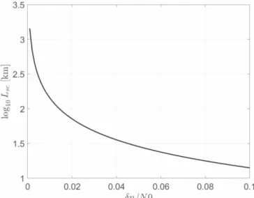
The characteristic scales of the density gradients obtained from synthetic density profiles are shown in Figure4. We start with dn N0=0.001, which results in Lsc∼103km. As one

can see, Lscdrops significantly with increasing levels of density

fluctuations, which in turn results in an increase of the efficiency of energy transformation from ES to EM waves. Thus, for δn/N0=0.1, which was measured onboard the

Helios satellite closer to the Sun (Bavassano & Bruno 1973),

the characteristic scale may be less than 15 km.

It is worth noting that the power spectrum used in this study is relevant for solar wind density fluctuations around 1 au. Closer to the Sun, the spectrum characteristics may be different, and as a result densityfluctuations can be described by the different statistics. In order to avoid speculations (though the method developed here is applicable), we consider emissions in the frequency range typical for a solar type III radio burst around 1 au: 10–100 kHz (Mann et al.1999).

Till now we considered the process of energy conversion only for primarily generated Langmuir waves, supposing that

the efficiency is proportional to the reflection coefficient Pref.

However, the very same process can operate when the reflected Langmuir wave undergoes the secondary reflection. This leads to the increase of the efficiency of energy conversion, which has a similar coefficient but the multiplierPref(1-Pref). As a summary, the factor that will take into account both processes will be (2Pref-Pref2 ).

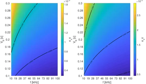
The conversion coefficient as a function of beam velocity, Vb, and the Langmuir wave frequency, f, are shown in Figure5.

The left panel shows Kefffor dn N0=0.1. As one can see for >

Vb 0.15c, the conversion coefficient is above ·5 10-4in the

whole range of frequencies. An increase of the level of the density fluctuations results in a decrease of the characteristic scale of the density gradient. As a result, reflection of the Langmuir waves will occur more often and Keffwill increase.

The right panel in Figure5shows Keff for dn N0=0.04. We found that the conversion coefficient is above ·5 10-4 _{in the} whole frequency range forVb>0.1c. For faster beams with

>

Vb 0.2c, the conversion coefficient is above 10−3 for

frequencies below 70 kHz.

Figure 3.Left panel: probability distribution function of the densityfluctuations. The blue line shows the distribution ofln¶n z( ) ¶zobtained from the synthetic profiles of the density fluctuations and the red line shows the fit of (Pln¶n z( ) ¶z)by Gaussian function. Right panel: probability distribution of the density gradients. The blue line shows the distribution obtained from the synthetic profiles and the red line shows the fit of this distribution by the function defined in Equation (13).

Figure 4.Characteristic scale of the densityfluctuations Lscas a function of the level of the densityfluctuations dn N0.

3. Effective Brightness Temperature

The notion of the effective brightness temperature is initially used to characterize an emissivity of an object, comparing it with the the emission of a blackbody in thermal equilibrium with its surroundings. It suggests that the energy distribution is close to the Planck law, or, for low frequencies and high temperatures, to the Rayleigh–Jeans law. If the wave’s spectral density distribution over frequencies is far from the distribution of the black or graybody then the very same notion is used to characterize either the spectral density of wave distribution or the total wave energy content. This concept is used in radio astronomy, planetary science, and materials science. Conven-tionally, the effective brightness temperature is determined using spectral intensity of the emission Ik, determined as an

energy of the emission with wave vectors k from unit volume in the k-space crossing the unit surface perpendicular to the vector of the group velocity Vgr= ¶ ¶w k. Following such a

definition (Zheleznyakov1977; Melrose1980)

p = D DW k T W k k 8 . b eff 3 2

It is widely used for characterization of the EM waves emission. For the Langmuir waves this notion may be used as an alternative characteristic similar to the total energy density of waves.

The beam relaxation process is described by the quasilinear equation, and represents the formation of the plateau-like distribution toward the lower velocities and an energetic tail. To estimate the energy transfer to Langmuir waves, one should evaluate the energy loss by particles. For the temporary problem it may be found from the balance of energyfluxes

D =

n mVb b Vb W .L

Here, DVb is the broadening of the electron distribution

function. The resonant conditions allow one to relate the width of the electron distribution function with the spectral width of the Langmuir waves spectral density. In the case of homogeneous plasma, it reads

w DV = D k k. b p res2

It was shown by Krasnoselskikh et al. (2011) that Langmuir

waves observed by Wind and Cluster satellites are distributed in the cone with the characteristic angleD , about 20° arounda the direction of the beam(which coincides with the direction of the background magneticfield). As such, solid angle DWLcan

be estimated as2p(1-cosDa), and the effective brightness temperature may be evaluated as

⎛ ⎝ ⎜ ⎞ ⎠ ⎟⎛ ⎝ ⎜ ⎞ ⎠ ⎟ ( ) ( ) ( ) p a p a w p a l = - D D = - D = - D k T W k k n mV n N E T N E 4 1 cos 4 1 cos 8 1 cos , b L L L L p b b b b e D b eff 2 4 2 3 5 2 0 3 2 0 3

where Eband nbare the kinetic energy and density of the beam,

respectively.

Studies of the beam–plasma instability in randomly inhomogeneous plasma, when the level of the density fluctuations is significantly higher than the effect of the wave dispersion, show that the major stage of the instability saturates at a significantly smaller level and the energy transferred to Langmuir waves is also significantly smaller. Moreover, the presence of the density fluctuations drastically changes the dynamics of the Langmuir turbulence. After a relevantly short period of growth WL reaches its maximum and then starts to

decay. Due to the broadening of the Landau resonance caused by the variations of the phase velocities of the waves, the waves can effectively exchange energy with electrons that have velocities higher then Vb and w kp 0. This leads to the acceleration of the electrons and decay of the wave energy density. Both the time of growth and time of decay of WLshow

dependence on the level of the densityfluctuations in a plasma. It is worth noting that such behavior of the Langmuir turbulence resembles a rise and decay of type III radio emission in the interplanetary medium. The detailed analysis of the dependence of the maximum energy level of Langmuir waves on the level of density fluctuations may be found in Voshchepynets et al. 2015and Voshchepynets & Krasnosels-kikh 2015. To take into account the effect of density fluctuations on the maximum wave energy, WL

max_{, that can be} gained in the process of beam relaxation, we introduce a dimensionless coefficient (r dn N0). The coefficient is defined

Figure 5.Conversion coefficient as a function of beam velocity Vband frequency of Langmuir waves f. Left panel: dn N0=0.01. Right panel: dn N0=0.04. The Astrophysical Journal, 879:51 (8pp), 2019 July 1 Krasnoselskikh, Voshchepynets, & Maksimovic

as a ratio of WmaxL for plasma with densityfluctuations to the

saturation level of the beam instability in homogeneous plasma (Vedenov & Ryutov1975). This ratio tends to decrease with an

increasing level of densityfluctuations, and its value is between 0.5 and 0.01 under conditions relevant for solar type III radio bursts (Voshchepynets et al.2015).

Thus, the effective brightness temperature will be written as follows ⎛ ⎝ ⎜ ⎞ ⎠ ⎟⎛ ⎝ ⎜ ⎞ ⎠ ⎟ ( ) ( ) p d a l = - D k T r n N n N E T N E 8 1 cos . b L b b e D b eff 2 0 0 3 2 0 3

The effective temperature of the EM (notified by symbol t (transverse)) can be determined as follows

p = D DW k T k W k 2 . b t t t t t eff 2 2

For EM waves, one can suggest Dkt=kt, thus

p = DW k T W k 2 , b t t t t eff 2 3

here DWt is the solid angle of angular distribution of EM

emission. The ratio of the effective temperatures is equal to = D DW D W = D DW DW T T W k k W k k W W k k k . t L t t t t L L L t t L L L t L t eff eff 2 2 2 3

Previously, we characterized the ratio of the energy density transferred to EM waves by the efficiency coefficient Keff.

Using it and making the reasonable assumption that D =kL 0.1kL, one can find the ratio of effective brightness

temperatures to be equal to ⎛ ⎝ ⎜ ⎞ ⎠ ⎟ = DW DW = DW DW = DW DW T T W W k k K k k K mc T 0.1 0.1 0.1 3 . t L L t t L L t L t L t L t e eff eff 3 3 eff 3 3 eff 2 3 2

Our previous analysis showed that the process of transfor-mation of ES waves into EM occurs in the narrow range of anglesYmax (Equation (9)). This implies a restriction on the angles of propagation of the EM emission

( ( ))

q<qmax=arcsinq_max1 2 c wLsc 1 3. This enables an estima-tion of the ratio DWL DWt as follows

a q DW DW = - D -1 cos 1 cos . L t max

Angle qmax is not necessarily small. For instance, in the plasma with dn N0=0.04, qmaxDa for the frequencies above 200 kHz. For the higher level of the densityfluctuations,

qmax can reach p 2 resulting in almost isotropic EM emission. Although, for dn N0<0.03, qmaxDaand DWL DW ~ 1t .

For solar wind plasma the multiplier (mc2 3T)3 2 _may become as large as 105, which can result in an effective brightness temperature of the EM emission comparable with the effective temperature of Langmuir waves when the transformation efficiency varies in the range of 10-6–10-5_. To evaluate characteristic values of the temperatures, let us take plasma and beam characteristics that correspond to intense solar radio bursts of type III: f_p =2 MHz,Eb=100 keV, Te=100 eV,nb N0=10-5, and (r dn N0)=1 10. Corresp-onding plasma density and Debye length are

 ´ - l 

N0 5 10 cm ,3 3 D 106 cm. In order to take into account the relativistic velocity of the beam, Equation (3)

should be rewritten as follows ⎛ ⎝ ⎜⎜ ⎞_⎠⎟⎟ ⎡_⎣⎢ ⎢ ⎛ ⎝ ⎜ ⎞_⎠⎟⎤ ⎦ ⎥ ⎥ ( ) ( ) d p a = - D - + k T E n c f r n N E E E 2 1 cos 1 , b L b p b eff 0 3 0 0 0 2 5 3

here E0=mc2 ~511 keV. In this case, the effective temper-ature of Langmuir waves is

 ´ ~ ´

k Tb effL 6 1013eV 7 1017K.

For the efficiency coefficient of the order of 10−3–10−4 (Figure5) the temperature ratio varies in the range 1–10; thus,

the EM temperatures, without taking into account the effects of damping along the propagation trajectory, varies as

–

1017 1018K_{. The values we obtain are significantly larger than} the typical brightness temperatures observed (Suzuki & Dulk1985; Saint-Hilaire et al.2013), but one should note that

the initially generated EM wave propagates toward the Sun, and before turning to the direction of the observer on the Earth, it undergoes multiple processes of scattering and reflection that correspond to quite strong absorption. The brightness temper-ature observed by an observer on the Earth should be significantly smaller, being described by the following expression

( )= ( ) (-G )

Tefft observed Tefft source exp L .

It is difficult to evaluate the result of such absorption, but angular broadening, as well as damping along the trajectory, may easily result in factors 10−3–10−4 (Li et al. 2008). The

measurements onboard the Parker Solar Probe and Solar Orbiter will allow us to evaluate these effects and to compare brightness temperatures directly measured in the source region observed distantly.

4. Conclusions

We show that the process of the linear conversion of Langmuir waves onto EM on random density fluctuations is effective under conditions relevant to solar wind. We show that this mechanism can result in the observed effective temperature of EM emission for solar radio bursts of type III in the order of1014–1015K_.

The efficiency of linear conversion is strongly dependent upon statistical properties of density fluctuations and their gradients. These characteristics may significantly vary with the distance from the Sun. The study of these dependencies comes beyond the scope of this paper and will be addressed in future publications.

V.K. acknowledges financial support by CNES through grant“Stereo-Waves invited scientist.”

ORCID iDs

Vladimir Krasnoselskikh https: //orcid.org/0000-0002-6809-6219

Andrii Voshchepynets https: //orcid.org/0000-0001-8307-781X

References

Alvarez, H., & Haddock, F. T. 1973,SoPh,30, 175

Celnikier, L. M., Muschietti, L., & Goldman, M. V. 1987, A&A,181, 138

Chen, C. H. K., Salem, C. S., Bonnell, J. W., Mozer, F. S., & Bale, S. D. 2012,

PhRvL,109, 035001

Denisov, N. G. 1957, JETP, 4, 544

Drummond, W. E., & Rosenbluth, M. N. 1962,PhFl,5, 1507

Ergun, R. E., Larson, D., Lin, R. P., et al. 1998,ApJ,503, 435

Ergun, R. E., Malaspina, D. M., Cairns, I. H., et al. 2008,PhRvL,101, 051101

Ginzburg, V. L., & Zhelezniakov, V. V. 1958, SvA,2, 653

Hinkel-Lipsker, D. E., Fried, B. D., & Morales, G. J. 1989,PhRvL,62, 2680

Hinkel-Lipsker, D. E., Fried, B. D., & Morales, G. J. 1991,PhRvL,66, 1862

Kellogg, P. J., Goetz, K., Monson, S. J., & Bale, S. D. 1999,JGR,104, 17069

Kontar, E. P. 2001,A&A,375, 629

Krafft, C., Volokitin, A. S., & Krasnoselskikh, V. V. 2013,ApJ,778, 111

Krafft, C., Volokitin, A. S., Krasnoselskikh, V. V., & de Wit, T. D. 2014,

JGRA,119, 9369

Krasnoselskikh, V. V., Dudok de Wit, T., & Bale, S. D. 2011,AnGeo,29, 613

Krasnoselskikh, V. V., Lobzin, V. V., Musatenko, K., et al. 2007,JGRA,112, A10109

Krupar, V., Maksimovic, M., Kontar, E. P., et al. 2018,ApJ,857, 82

Li, B., Cairns, I. H., & Robinson, P. A. 2008,JGRA,113, A06104

Lin, R. P., Potter, D. W., Gurnett, D. A., & Scarf, F. L. 1981,ApJ,251, 364

Malaspina, D. M., Cairns, I. H., & Ergun, R. E. 2012,ApJ,755, 45

Malaspina, D. M., & Ergun, R. E. 2008,JGRA,113, A12108

Mann, G., Jansen, F., MacDowall, R. J., Kaiser, M. L., & Stone, R. G. 1999, A&A,348, 614

Melrose, D. B. 1980, Plasma Astrohysics. Nonthermal Processes in Diffuse Magnetized Plasmas; Vol. 2: Astrophysical Applications(London: Gordon and Breach)

Melrose, D. B. 1987,SoPh,111, 89

Melrose, D. B. 1990,SoPh,130, 3

Melrose, D. B. 2017,RvMPP,1, 5

Piliya, A. D. 1966, SPTP, 11, 609

Píša, D., Hospodarsky, G. B., Kurth, W. S., et al. 2015,JGRA,120, 2531

Reid, H. A. S., & Kontar, E. P. 1995,PhPl,2, 1466

Reid, H. A. S., & Kontar, E. P. 2013,SoPh,285, 217

Reid, H. A. S., & Kontar, E. P. 2017,A&A,598, A44

Reid, H. A. S., & Kontar, E. P. 2018,A&A,614, A69

Robinson, P. A., Cairns, I. H., & Gurnett, D. A. 1993,ApJ,407, 790

Romanov, Y. A., & Filippov, G. F. 1961, JETP, 13, 87 Saint-Hilaire, P., Vilmer, N., & Kerdraon, A. 2013,ApJ,762, 60

Smith, D. F., & Sime, D. 1979,ApJ,233, 998

Stenzel, R. L., Wong, A. Y., & Kim, H. C. 1974,PhRvL,32, 654

Suzuki, S., & Dulk, G. A. 1985, in Solar Radiophysics, ed. D. J. McLean & N. R. Labrum(Cambridge: Cambridge Univ. Press),289

Vedenov, A. A. 1963,JNuE,5, 169

Vedenov, A. A., & Ryutov, D. D. 1975, RvPP,6, 1

Vidojevic, S., Zaslavsky, A., Maksimovic, M., et al. 2012, PASRB,11, 343

Volokitin, A. S., & Krafft, C. 2018,ApJ,868, 104

Voshchepynets, A., & Krasnoselskikh, V. 2015,JGRA,120, 10

Voshchepynets, A., Krasnoselskikh, V., Artemyev, A., & Volokitin, A. 2015,

ApJ,807, 38

Voshchepynets, A., Volokitin, A., Krasnoselskikh, V., & Krafft, C. 2017,

JGRA,122, 3915

Wild, J. P., & McCready, L. L. 1950,AuSRA,3, 387

Zaslavsky, A., Volokitin, A. S., Krasnoselskikh, V. V., Maksimovic, M., & Bale, S. D. 2010,JGRA,115, A08103

Zheleznyakov, V. V. 1977, Electromagnetic Waves in Cosmic Plasma: Generation and Propagation(Moscow: Nauka)