HAL Id: hal-00318357
https://hal.archives-ouvertes.fr/hal-00318357
Submitted on 30 Jul 2007
HAL is a multi-disciplinary open access
archive for the deposit and dissemination of
sci-entific research documents, whether they are
pub-lished or not. The documents may come from
teaching and research institutions in France or
abroad, or from public or private research centers.
L’archive ouverte pluridisciplinaire HAL, est
destinée au dépôt et à la diffusion de documents
scientifiques de niveau recherche, publiés ou non,
émanant des établissements d’enseignement et de
recherche français ou étrangers, des laboratoires
publics ou privés.
variances and solar wind correlations
M. Förster, G. Paschmann, S. E. Haaland, J. M. Quinn, R. B. Torbert, H.
Vaith, C. A. Kletzing
To cite this version:
M. Förster, G. Paschmann, S. E. Haaland, J. M. Quinn, R. B. Torbert, et al.. High-latitude plasma
convection from Cluster EDI: variances and solar wind correlations. Annales Geophysicae, European
Geosciences Union, 2007, 25 (7), pp.1691-1707. �hal-00318357�
www.ann-geophys.net/25/1691/2007/ © European Geosciences Union 2007
Annales
Geophysicae
High-latitude plasma convection from Cluster EDI: variances and
solar wind correlations
M. F¨orster1, G. Paschmann2, S. E. Haaland2,3, J. M. Quinn4, R. B. Torbert5, H. Vaith2, and C. A. Kletzing6
1GeoForschungsZentrum Potsdam, Potsdam, Germany
2Max-Planck-Institut f¨ur extraterrestrische Physik, 85748 Garching, Germany 3Department of Physics, University of Bergen, Norway
4Boston University, Boston, MA 02215, USA
5University of New Hampshire, Durham, NH 03824, USA
6University of Iowa, Iowa City, IA 52242, USA
Received: 14 March 2007 – Revised: 21 June 2007 – Accepted: 16 July 2007 – Published: 30 July 2007
Abstract. Based on drift velocity measurements of the EDI instruments on Cluster during the years 2001–2006, we have constructed a database of high-latitude ionospheric convec-tion velocities and associated solar wind and magnetospheric activity parameters. In an earlier paper (Haaland et al., 2007), we have described the method, consisting of an im-proved technique for calculating the propagation delay be-tween the chosen solar wind monitor (ACE) and Earth’s mag-netosphere, filtering the data for periods of sufficiently stable IMF orientations, and mapping the EDI measurements from their high-altitude positions to ionospheric altitudes. The present paper extends this study, by looking at the spatial pat-tern of the variances of the convection velocities as a function of IMF orientation, and by performing sortings of the data ac-cording to the IMF magnitude in the GSM y-z plane, |ByzIMF|, the estimated reconnection electric field, Er,sw, the solar
wind dynamic pressure, Pdyn, the season, and indices
char-acterizing the ring current (Dst) and tail activity (ASYM-H).
The variability of the high-latitude convection shows charac-teristic spatial patterns, which are mirror symmetric between the Northern and Southern Hemispheres with respect to the IMF By component. The latitude range of the highest
vari-ability zone varies with IMF Bz similar to the auroral oval
extent. The magnitude of convection standard deviations is of the same order as, or even larger than, the convection mag-nitude itself. Positive correlations of polar cap activity are found with |ByzIMF|and with Er,sw, in particular. The strict
linear increase for small magnitudes of Er,sw starts to
devi-ate toward a flattened increase above about 2 mV/m. There is also a weak positive correlation with Pdyn. At very small
values of Pdyn, a secondary maximum appears, which is even Correspondence to: M. F¨orster
more pronounced for the correlation with solar wind proton density. Evidence for enhanced nightside convection during high nightside activity is presented.
Keywords. Ionosphere (Plasma convection) – Magneto-spheric physics (MagnetoMagneto-spheric configuration and dynam-ics; Solar wind-magnetosphere interactions)
1 Introduction
Large spatial and temporal variability is a fundamental prop-erty of magnetospheric convection. This is mainly caused by variations in the driving solar wind and interplanetary magnetic field (IMF) conditions together with the complex-ity of the coupled system. Competing time-dependent pro-cesses are acting with various characteristic time scales such that steady-state conditions therefore rarely exist and any re-sponse to changes in various interplanetary conditions for any given moment in time depend further on the prior state of the system (Rostoker et al., 1988). The major part of the transfer of energy and momentum from the solar wind to Earth’s magnetosphere and the basic high-latitude convec-tion patterns are now known to be caused by reconnecconvec-tion between the IMF and Earth’s geomagnetic field (Dungey, 1961) and to a minor extent by quasi-viscous interaction pro-cesses at the magnetopause (Axford and Hines, 1961). Dur-ing periods when IMF has a southerly component, reconnec-tion takes place on the dayside magnetopause. The newly reconnected field lines and the plasma attached to them are swept across the polar caps into the magnetotail where they eventually reconnect again. Both of these two basic time-dependent components of the magnetospheric convection cy-cle can be reasonably parametrized in terms of the concurrent
0 2 4 6 0 2.0•103 4.0•103 6.0•103 8.0•103 1.0•104 1.2•104 Pdyn [nPa] 0 -50 -100 0 2.0•103 4.0•103 6.0•103 8.0•103 1.0•104 1.2•104 Dst [nT] 0 20 40 60 80 100 0 5.0•103 1.0•104 1.5•104 ASYM_H [nT] 0 2 4 6 8 10 12 14 0 2000 4000 6000 8000 | ByzIMF | [nT] 300 400 500 600 700 800 0 2.0•103 4.0•103 6.0•103 8.0•103 1.0•104 1.2•104 | Vsw | [km/s] -1.5 -1.0 -0.5 0.0 0.5 1.0 0 2000 4000 6000 8000 log E r sw [mV/m] -180 -90 0 90 180 0 1000 2000 3000 4000 5000
clock angle [deg]
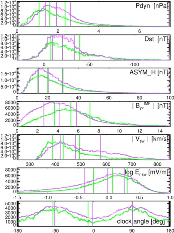
Fig. 1. Solar wind and geomagnetic parameter distribution for the
time interval of EDI observations 2001–2006. All data points used for the analysis, i.e., after filtering for stable IMF conditions, are drawn as green lines; the purple lines illustrate the contrasting data set of all those data points that were removed by the filtering. The panels from top to bottom show the dynamic pressure of the so-lar wind protons, Pdyn, at the magnetopause, the Dst index
char-acterizing geomagnetic activity of the ring current, the ASYM-H index which is used here as a proxy of the AE index of auroral ge-omagnetic activity, the magnitude of the IMF vector components in the GSM y-z-plane, |ByzIMF|, the magnitude of solar wind velocity,
|Vs.w.|, the solar wind reconnection electric field, Er,sw(see Eq. 3),
and finally the IMF clock angle. The vertical lines in each panel indicate the quartiles of the distribution for the corresponding pa-rameter.
near-Earth interplanetary conditions, although with different response times (Cowley and Lockwood, 1992). For north-ward IMF, reconnection takes place at high latitudes between the IMF and Earth’s lobe field (see, e.g., Burke et al., 1979; Reiff and Burch, 1985; Reiff and Heelis, 1994).
The result of these processes is a large scale circulation of plasma in Earth’s magnetosphere. Since the geomagnetic field lines are nearly equipotentials, and the large scale cir-culation map to high magnetic latitudes, this plasma circula-tion and its variability is also manifested in the high latitude ionosphere. In addition, the ionosphere itself and the ther-mosphere where it is embedded play a role. Sunlight and
particle precipitation enhances the ionospheric conductivity leading to an attenuation of the electric field, and the iono-sphere, being tightly coupled to the thermoiono-sphere, acts as a “drag” on convection (Cole, 1963; Hill, 1976). The high-latitude convection and its variability in particular also play a major role in Joule heating of the ionosphere and thermo-sphere. Joule heating is generated due to relative motions of the neutral gas and ionized components, being propor-tional to the square of the velocity difference. The contri-bution of the irregular part of the convection has been shown to be comparable to or in certain regions even larger than the Joule heating of the averaged or background convection. It is as an essential contributor of thermospheric energy at high latitudes (Codrescu et al., 1995, 2000; Crowley and Hackert, 2001). The inertia of the thermospheric neutral winds can help to maintain the ionospheric convection independently of the magnetospheric driver processes and is known as the fly-wheel effect (Banks, 1972; Coroniti and Kennel, 1973). Taken together, the convection patterns are thus caused by the combined effect of several processes rather than a single elementary process (Tanaka, 2001). Statistical dependencies of the solar wind drivers such as the IMF and the solar wind dynamic pressure, have been studied extensively for several decades (e.g., Reiff et al., 1981; Heppner and Maynard, 1987; Boyle et al., 1997).
In an earlier paper (Haaland et al., 2007), henceforth re-ferred to as Paper 1, the statistical pattern of high-latitude (magnetic latitudes >58◦) ionospheric convection as a func-tion of the IMF clock angle, deduced from measurements by the Electron Drift Instruments (EDI) onboard the Clus-ter satellites during the years 2001–2006, was presented. Paper 1 describes the method, consisting of an improved technique for calculating the propagation delay between the solar wind monitor, the Advanced Composition Explorer (ACE), and Earth’s magnetosphere, filtering the data for pe-riods of sufficiently stable IMF orientations, and mapping the EDI measurements from their high-altitude positions to iono-spheric altitudes. In Paper 1 we sorted the data according to the IMF orientation, averaged the data, and generated maps of the potential distribution. In the present paper we use the same comprehensive data set to investigate the dependencies of high-latitude convection on various other solar wind and magnetospheric activity parameters. We also discuss the spa-tial pattern of the variances of the convection velocities.
2 Data set characteristics
In order to characterize the data set, Fig. 1 shows the distribu-tions of the selected solar wind parameters over the time-span of our data set: clock angle θ , magnitude of the IMF in the GSM (y,z)-plane |ByzIMF|(sometimes called BT or “transverse
IMF magnitude”), the solar wind speed |Vs.w.|, the magnitude
of the solar wind electric field projected along the reconnec-tion line at the dayside magnetopause, Er,sw, and dynamic
pressure Pdynof solar wind protons (including heavier ions
like alpha particle gives on average about 20% higher val-ues). The parameters were derived from measurements at ACE as described in Paper 1. Figure 1 also shows the dis-tribution of two geomagnetic indices (Dstand ASYM-H)
as-sembled together with the solar wind and IMF parameters with the same 1-min resolution. The solar wind parameters have been shifted for arrival time at the magnetopause (as-sumed to be located at XGSE=10 RE).
The method described in Paper 1 used a bias vector filter-ing to select relatively stable IMF conditions for well-defined magnetospheric convection response patterns as a function of the IMF clock angle in eight discrete sectors with 45◦width each. IMF sector 0 is purely northward (IMF Bz+) directed,
the other sectors follow clockwise in the IMF y-z plane, so that IMF sectors 2 and 6 correspond to By+ and By–,
re-spectively, and sector 4 is close to strict southward direction (IMF Bz–). This selection process resulted in a filtered data
set which comprises nearly half the full data set originally available. However, the IMF stability filtering might have biased the characteristic solar wind conditions in a system-atic manner. To check this, we plotted in Fig. 1 not only the distributions of the data set with stable IMF conditions used for our study (green lines), but also the complementary ones, i.e., the distributions for all rejected data points (purple lines). The vertical lines indicate the quartiles of the distri-bution.
Differences between the two data sets are clearly seen in the solar wind parameter Pdyn, the IMF magnitude |ByzIMF|,
and the solar wind velocity |Vs.w.|. The discarded data points
are characterized by larger average solar wind speed and therefore larger mean Pdyn values while the proton density
distribution (not shown) is generally not influenced. The Dst
index becomes more concentrated within the range −10 nT to −35 nT under disturbed IMF conditions while the partial ring current activity index ASYM-H as well as the average clock angle distribution of the IMF vectors do not show any significant difference.
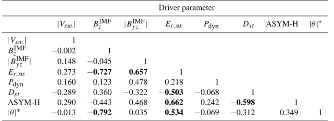
The parameters we have chosen for our secondary sort-ings are not independent of the IMF clock angle that we used to sort the data in Paper 1, and they are also somewhat de-pendent on each other. This is illustrated by Table 1. For a significance test of the correlation coefficients we used the Student’s t-distribution. Due to the large number of data points, all correlation coefficients estimated can be regarded as statistically reliable. Their significance in a pure statis-tical sense is already gained for values above ≈0.01. The quality of correlation, on the other hand, is given by the cor-relation coefficient itself with its range from −1.0 to +1.0; larger magnitudes indicate stronger correlations. To guide the reader, we highlighted in Table 1 all coefficients with magnitudes >0.5.
The clear anticorrelation between BzIMFand the absolute value of the clock angle |θ | results simply from its definition as function of ByIMFand BzIMF. A further clear anticorrelation
40 60 80 100 120 140 0 500 1000 1500 2000 2500
3000 North HemisphereSouth Hemisphere
Number of records
solar zenith angle [deg]
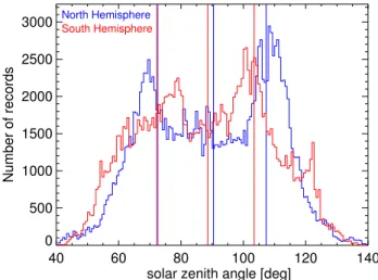
Fig. 2. Solar zenith angle distributions at the ionospheric footpoint
location of the mapped EDI drift vectors in the ionosphere for North (blue) and South (red) Hemisphere separately. The vertical lines indicate the quartiles of the distributions.
exists between the geomagnetic indices Dst and ASYM-H;
declining ring current values of disturbed periods are related to a rising auroral activity. All other high correlation values concern the reconnection electric field parameter of the solar wind Er,sw, except for its relation to Pdyn and |Vs.w.|. There
are also some smaller, but noticeable correlations of ASYM-H with BIMF
z and |ByzIMF|. All other pairs of parameters are
uncorrelated.
The line of apsides of the Cluster orbit, originally equa-torial, is tilting further and further southward with time. In our data set, there is therefore an asymmetry in the North-South coverage within the high magnetic latitudes regions. This manifests itself, for example, in different seasonal cov-erages at the Northern and Southern Hemisphere (see Fig. 5 in Paper 1, middle and bottom panels). Also, Southern Hemi-sphere data are on average obtained at higher altitudes (9 RE
versus 7 RE for the Northern Hemisphere). However, the
Southern Hemisphere data contain a larger fraction of ob-servations taken during sunlit conditions. This is probably due to a clear difference in the offsets between the geo-graphic and geomagnetic poles at the North and South Hemi-sphere. Based on the International Geomagnetic Reference Field (IGRF) model, the 2005 location of the north magnetic pole is 83.21◦N and 118.32◦W and the south magnetic pole
is 64.53◦S and 137.86◦E. The larger displacement at the
Southern Hemisphere leads to a larger diurnal “wobbling” of the polar cap area with respect to the geographic coordinates. Figure 2 shows the number of observations for the Northern (blue lines) and Southern (red lines) Hemisphere versus solar zenith angle. Zenith angles below approximately 100◦ cor-responds to a sunlit polar cap ionosphere and thus enhanced ionization and subsequent attenuation of the electric field. As already pointed out by Cole (1963) and Hill (1976), a higher
Table 1. Correlations between the various driver parameters (using all bias-filtered data).
Driver parameter
|Vs.w.| BzIMF |ByzIMF| Er,sw Pdyn Dst ASYM-H |θ |∗
|Vs.w.| 1 BzIMF −0.002 1 |ByzIMF| 0.148 −0.045 1 Er,sw 0.273 −0.727 0.657 1 Pdyn 0.160 0.123 0.478 0.218 1 Dst −0.289 0.360 −0.322 −0.503 −0.068 1 ASYM-H 0.290 −0.443 0.468 0.662 0.242 −0.598 1 |θ |∗ −0.013 −0.792 0.035 0.534 −0.069 −0.312 0.349 1
∗absolute values of the clock angle used.
ionospheric conductivity will retard the convection due to the drag force caused by ion-neutral collisions. Since the mag-netic field lines are nearly equipotentials, the effect of this drag is also observed at Cluster altitudes. Due to the asym-metry, the average convection velocities obtained within the Southern polar cap are slightly lower (≈7%) than those from the Northern Hemisphere. This difference is smaller within the very central part of the polar cap, where the mapped EDI drift data have best coverage.
3 Convection variability
In Paper 1, we have presented the average convection pat-terns as a function of IMF direction without any considera-tions of variability. But as noted earlier, the convection pat-tern is known to be highly variable on different timescales. Variations on timescales of minutes are known even for rela-tively stable IMF conditions (Bristow et al., 2004).
To characterize the variability of the convection in our sta-tistical study of EDI drift measurements, we used two dif-ferent variances. Normalized to the average drift magnitude, they are defined as follows:
σtotal2 = h|v| 2i − |hvi|2 h|v|2i (1) σmag2 = h|v| 2i − h|v|i2 h|v|2i (2)
where h...i denotes average over time and v is the velocity vector. The first variance, σtotal2 , is the normalized variance (equivalent to the sum over the component variances) of the total velocity vector. It represents the variability of the full vector, with a steady pointing direction yielding zero vari-ance. The second variance, σmag2 , is the normalized variance of the velocity magnitude, and gives the average deviation of the velocity magnitude from its local average value. Both variances range from 0 to 1.
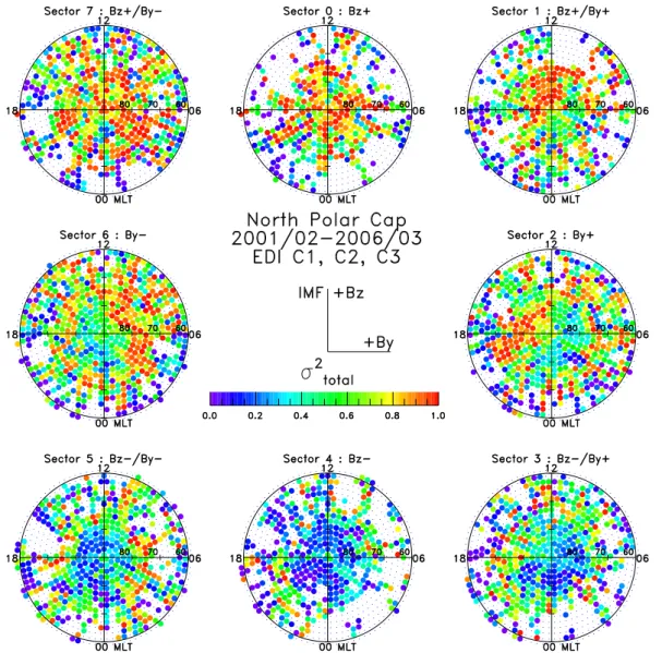
The normalized total drift velocity variance, σtotal2 , is shown in Figs. 3 and 4 for the Northern and Southern Hemi-sphere, respectively. The eight panels are for different clock angle ranges (corresponding to those in Paper 1) and reveal a systematic pattern of the drift variance over the whole po-lar cap as a function of the IMF clock angle. The variability approaches 1 over large areas in a systematic way. For the three sectors of northward IMF (upper row), this enhanced variability fills nearly the whole polar cap region, while for southward IMF (bottom panels), the variance is small within the polar cap.
The ByIMFdominated sectors (2 and 6) show a dawn-dusk asymmetry in the maximum intensities of the normalized variance. The normalized variance at the Northern Hemi-sphere (Fig. 3) shows high values at the dusk (dawn) side for positive (negative) ByIMFvalues. The dayside quadrant at the dusk (dawn) side is completely covered while this en-hanced normalized variance is confined to about 20:00 MLT (03:00 MLT) on the nightside. Note that regions inside the polar cap with normalized variances close to 1 have lower average convection velocities. They correspond to the round-shaped convection cells areas with wider spaced potential contours (see Figs. 7 and 8 in Paper 1). For northward IMF, somewhat broader regions of more enhanced variability are seen on the dayside as, e.g., in sector 1 of Fig. 3 and sector 7 of Fig. 4.
Inside the polar cap region, there is a region of more struc-tured flow (smaller normalized variances and more ’bundled’ convection stream lines) which broadens for further south-ward turning of the IMF as seen in the lower row (sectors 3– 5). For purely southward IMF (Sector 4), the well-organized transpolar flow covers the entire polar cap region down to nearly 70◦. Further equatorward, in the convection reversal zone and return flow, the variance is higher than in the central polar cap again. The diameter of the low-variance region in the central polar cap becomes smaller for northward turning IMF.
Fig. 3. Total normalized variance of the EDI drift vectors mapped to the Northern high latitude ionosphere for the time interval from February
2001 to March 2006. The outer circle of each panel represents 60◦magnetic latitude and the numbers indicate magnetic local time (MLT). The color bar shows the intensity of the variability; the normalized values are confined to an interval between 0 and 1. The variance is calculated for each bin individually, based on at least three valid mapped drift vectors within the bin.
Comparing the Southern Hemisphere (Fig. 4) with the Northern (Fig. 3), the patterns are mirror symmetric with re-spect to the ByIMFdependence, that is, there are high values of normalized variance at the dawn (dusk) side for positive (negative) ByIMFvalues, respectively. All other differences are minor as, e.g., an apparently broader ring of enhanced vari-ability at auroral and subauroral latitudes on the nightside for southward IMF.
The other normalized variance, σmagn2 (not shown here), reveals similar patterns of variability with the same ByIMFdependence, but on a much lower level of amplitudes. Its maximum magnitudes reach only about half of those of the total variance.
Figures 3 and 4 were for the normalized variances. To em-phasize the absolute variations, Fig. 5 shows the standard de-viation of the full vector for the Northern Hemisphere, with-out any normalization.
The auroral oval (convection reversal zone) and its dia-meter change with varying BzIMFvalues is clearly reflected in these patterns. For sector 0 (purely northward IMF), this oval has its smallest radial extent and the region of enhanced standard deviation values is nearly closed throughout the po-lar cap. This oval gradually extends for the other sectors with a maximum diameter low values (more ordered convection) within the polar cap for sectors 3–5 under southward IMF conditions. The absolute values within the auroral oval are of the order of the average drift velocity and are marked by the
Fig. 4. As in Fig. 3, but for the Southern Hemisphere.
range of the colour scale chosen (about 700 m s−1). Within
the auroral oval inside the central polar cap the standard devi-ations have about half of this magnitude (around 350 m s−1). The ByIMFdependence that was apparent in the normalized variances is not seen here in the standard deviation plot.
On the nightside, there is a tendency for enhanced values in the evening to midnight magnetic local times, in particular for southward IMF, extending toward early morning hours (≈02:00 MLT) as can be seen in sector 5 (this cannot be con-firmed for sectors 3 and 4 due to scarcity of mapped EDI drift vectors in this area). This might be due to enhanced substorm activity.
While Figs. 3–5 characterize the variability in terms of normalized variances and unnormalized standard deviations, Fig. 6 shows time series of the XSM component of all
avail-able EDI velocity data that are mapped into the central polar cap region poleward of 80◦ magnetic latitude, divided into
four different main IMF directions corresponding to the four 90-deg quadrants of IMF clock angle. Particular striking is that there is a large variability down to very short time scales, in particular for northward IMF (quadrant 0 – top panel), but also for IMF directions in the ecliptic plane (quadrants 1 and 3). For southward IMF (quadrant 2) the variability is much lower, and comparable to or even smaller than the average drift vector magnitude (see the red lines in Fig. 6). Table 2 lists additionally the mean values and standard deviations of the the boxcar averages shown in Fig. 6. Note also that there are no long-term trends of the averages.
4 Solar wind dependencies
To investigate the influence on the convection of various so-lar wind and IMF quantities, such as the soso-lar wind dynamic pressure Pdyn, the solar wind electric field Er,sw, the IMF
Fig. 5. Standard deviation of the total vector variation [m s−1] of EDI drift vectors mapped to the Northern high latitude ionosphere for the time interval from Feb 2001 to Mar 2006. As in Figs. 3 and 4, each circular panel shows magnetic local time (MLT) versus magnetic latitude with 60◦at the outer border. The color bar indicates the magnitude of the standard deviation, which is calculated for each bin individually, based on at least three valid mapped drift vectors within the bin.
magnitude |ByzIMF|, and the Dst index, we bin our data set
into a number of subsets for each of these parameters. The binning is a compromise between adequate resolution and sufficient data coverage. A good and homogeneous cover-age is particularly important for the construction of the po-tential patterns. Large gaps in the longitudinal or latitudinal coverage cause problems with the Legendre polynomial ex-pansion, which can lead to artifacts in the potential distribu-tion (see Sect. 3.5 in Paper 1). For this reason, we calculate the average convection velocity within the central polar cap (magnetic latitude |φm|>80◦) for each subset. Note that this
selected area typically does not include the low latitude re-gions of convection return flow.
In the following, we use the magnitude of the average ve-locity components hVxiand hVyias measures for the
mag-netospheric convection velocity across the center polar cap as well as hV i, which represents the average of the veloc-ity magnitudes. Vx, Vy and Vz are the mapped EDI drift
velocity components at ionospheric level (400 km) in Solar Magnetic (SM) coordinates (Vz is usually very small in the
high-latitude ionosphere). Note that the antisolar velocity is plotted with an inverted sign (h−Vxi) in the following figures
of this section for better comparison with hV i dependencies.
4.1 IMF direction
Figure 7 shows the cross-polar cap potential (upper panel) as well as the average velocities defined above versus clock
-4 -2 0 2 4 Vx_SM (km/s) Quadrant 0 -4 -2 0 2 4 Vx_SM (km/s) Quadrant 1 -4 -2 0 2 4 Vx_SM (km/s) Quadrant 2 -4 -2 0 2 4 Vx_SM (km/s) 2001 2002 2003 2004 2005 MLAT > 80 deg Both hemispheres Quadrant 3
Fig. 6. 62 months of mapped EDI drift measurements in XSM
direction within the central polar cap region (magnetic latitude
|φm|>80◦), plotted as condensed time series for the four different
quadrants of the IMF clock angle distribution. As indicated with the small circle inlet for each respective panel, quadrant 0 of clock angle distribution comprises ±45◦centered around 0◦clock angle, quad-rant 1 the same angular width centered around 90◦, and so forth. Boxcar averages (6 month centered window) are shown as red lines and their standard deviations are indicated by the dashed red lines.
Table 2. Average values of the sliding boxcar mean values for 62
months of mapped EDI drift measurements in XSM direction (red
lines in Fig. 6) and their average standard deviations for each quad-rant of the IMF clock angle distribution individually.
Quadrant IMF Mean value STDDEV direction m/s m/s
0 Bz+ +4 506
1 By+ −252 420
2 Bz− −544 308
3 By− −317 414
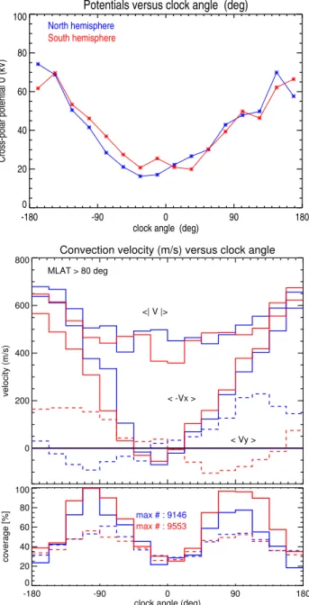
angle in 16 steps of 22.5◦each (middle panel) and the corre-sponding spatial coverage (lower panel). This figure comple-ments Figs. 7 and 8 in Paper 1, but has twice the resolution in clockangle. The cross-polar cap potential is derived from po-tential pattern that were constructed with all data points of the
Potentials versus clock angle (deg)
-180 -90 0 90 180
clock angle (deg) 0 20 40 60 80 100 Cross-polar potential U (kV) North hemisphere South hemisphere
Convection velocity (m/s) versus clock angle
0 200 400 600 800 velocity (m/s) <| V |> < -Vx > < Vy > -180 -90 0 90 180
clock angle (deg) 0 20 40 60 80 100 coverage [%] max # : 9146 max # : 9553 MLAT > 80 deg
Fig. 7. Top: Polar cap potentials as a function of clock angle for the
Northern (blue) and Southern (red) Hemisphere. The clock angle range is divided in 16 steps of equal width (22.5◦). The potentials in this panel are derived from the full high-latitude (>58◦) convec-tion pattern for each bin, as explained in Paper 1. Middle: The av-erage convection velocities hV i, h−Vxi, and hVyi(dashed) within
the central polar cap at magnetic latitudes |φm|>80◦as function
of clock angle, using the same colour coding and bin-step widths as above. Bottom: coverage characteristics for each bin individu-ally. The solid lines, which refer to the middle panel, show the rela-tive number of data points within the high-latitude circle (>80◦) for each bin, as percentage of the maximum number noted within the panel. The dashed lines refer to the upper panel, indicating the per-centage of valid grid points of the full area of the polar cap potential pattern construction.
bin-step interval as explained in Sect. 3.5 of Paper 1. The po-tential difference between the maximum and minimum value of the potential pattern is used for the curves in the upper panel. In most cases, this co-incides with the cross-polar cap potential difference between the main cells, the positive fo-cus of the dawn cell and the negative of the dusk cell.
The figure confirms the rough mirror symmetry between North and South as well as the remaining minor hemispheric differences. There are different minimum positions of the po-tentials for North and South close to zero degree clock angle (BzIMF+) in the upper panel. The Northern Hemisphere shows a smooth broad minimum slightly shifted toward negative clock angles while at the Southern Hemisphere this minimum near 0◦clock angle is less clear and seems rather shifted to-ward positive values.
At southerly clock angles the two curves of hV i and the two curves h−Vxi in the middle panel of Fig. 7 are close,
which means that the velocity directions are rather steady in antisolar direction over the central polar cap. This indicates that the contribution of hVyi (dashed), being approximately
mirror symmetric between North and South with respect to 0◦clock angle, is negligible. By contrast, at northerly clock-angles the hV i and h−Vxicurves are quite far apart and hVyi
is comparable to hVxi, indicating that the directions are less
steady: averaging the magnitudes then gives a large value for hV i, while the variable directions causes partial compensa-tion in the individual components. hVxieven becomes
pos-itive on average for values near 0◦ clock angle (northward IMF). This is due to the appearance of lobe cells with sun-ward convection at high latitudes. The minimum value of h−Vxi is slightly shifted toward negative clock angles for
both Northern and Southern Hemisphere. This behaviour is similar to the potential variation in the upper panel result-ing in steeper variation in the range of negative clock angles compared to the positive half-sphere.
The averaged convection velocity (middle panel of Fig. 7) reveals some North-South asymmetry, particularly in hV i and h−Vxi (when mirrored the southern curve at 0◦ clock
angle). This is presumably partially a result of the conduc-tivity differences discussed in Sect. 2, but mainly the result of the mirror-symmetric action of the ByIMFdependence. Devia-tions of the geomagnetic field configuration from symmetry, in particular at ionospheric altitudes, will probably also affect the results (see also the discussion later in Sect. 4.5). 4.2 Effect of IMF magnitude |ByzIMF|
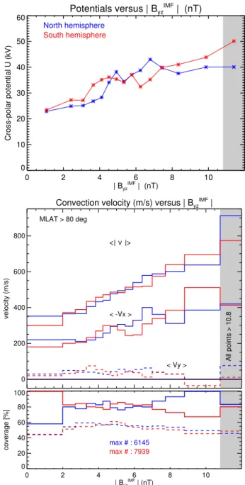
In a recent paper, Ruohoniemi and Greenwald (2005), ex-amined the influence of the IMF magnitude in the GSM y-z plane (|ByzIMF|) on the convection patterns. They divided the IMF magnitude |ByzIMF| into three bins: 0–3 nT, 3–5 nT and 5–10 nT, and found that higher values of |ByzIMF| corre-spond to higher polar cap potentials. The only exception was found for pure northward IMF, where the polar cap potential remained fairly low and stable. For northward IMF values
Potentials versus | Byz IMF | (nT) 0 2 4 6 8 10 | Byz IMF | (nT) 0 10 20 30 40 50 60 Cross-polar potential U (kV) North hemisphere South hemisphere
Convection velocity (m/s) versus | ByzIMF |
0 200 400 600 800 velocity (m/s) < -Vx > < Vy > All points > 10.8 0 2 4 6 8 10 | Byz IMF | (nT) 0 20 40 60 80 100
coverage [%] max # : 6145max # : 7939
MLAT > 80 deg
Fig. 8. Top: Polar cap potentials derived from the full high-latitude
convection pattern for each bin as a function of |ByzIMF|for the Northern (blue) and the Southern Hemisphere (red). Middle panel: Average velocities as a function of the IMF magnitude |ByzIMF|
within the central polar cap at magnetic latitudes |φm|>80◦only.
Lower panel: coverage for each bin as explained in Fig. 7, except that we now used variable bin widths so that the amount of data points are about equal in each bin-step.
in the 5–10 nT range, they also found signatures of sunward convection and the emergence of lobe cells in the high lati-tude dayside polar cap. |ByzIMF|is one of the parameters that determines the solar wind electric field and is thus expected to influence the cross polar cap potential.
To perform a similar analysis, we have combined all IMF directions, but divided the parameter range into more bins. These bin-steps were chosen such that they contain about the same amount of data – the steps are therefore not equidistant in contrast to the previous figure. The number of the steps was chosen such that the number of data points in each bin is sufficient for the velocity averages, and guarantees at the same time a good grid point coverage for the polar cap poten-tial pattern, which results in 15 non-equal steps. The result-ing coverage is illustrated in the bottom panel of Fig. 8. The full lines show the relative number of data points in each bin as percentage of the maximum number for the Northern and Southern Hemispheres separately. The deviations from the maximum number and the varying relative coverage between North and South is due to small hemispheric differences. The dashed lines show the percentage of valid grid points within the full area for the polar cap potential pattern construction (see Paper 1, Sect. 3.5) which is used for the upper panel.
The upper panel of Fig. 8 shows the derived cross-polar cap potential as a function of |ByzIMF|for both the Northern (blue line) and Southern Hemisphere (red line). They show the same positive trend, although there are some non-regular variations in the middle range from about 3 nT to 7 nT. For small magnitudes of |ByzIMF|∼< 3 nT, the cross-polar cap po-tential has a minimum value between about 20 kV to 25 kV. Up to about 10 nT, there is a positive correlation, in agree-ment with Ruohoniemi and Greenwald (2005). For |ByzIMF| values above the range shown in Fig. 8, the potential con-struction suffers from poor spatial coverage. The last step, marked with grey shading, contains therefore all data points above ≈10.8 nT.
The middle panel of Fig. 8 shows the dependence on |ByzIMF| of the convection velocities hV i, h−Vxi, and hVyi.
As already mentioned above, these averages are derived with data points from the central polar cap area (at |φm|>80◦).
The binning of the whole parameter range is the same as for the potential pattern in the upper panel. The velocities in the middle panel, particularly h−Vxi, show approximately
the same dependence on |ByzIMF|as the cross-polar cap poten-tial in the upper panel, including the minor variations in the middle range. It can therefore be regarded to some extent as a proxy for the cross-polar cap potential. This will be uti-lized further in subsequent sections. The proxy character is not surprising given that v=E×B/B2and B is essentially constant within the auroral oval. While h−Vxirepresents the
localized dawn-dusk electric field strength within the central polar cap, the polar cap potential stands for the larger-scale, integrating effect of the solar wind–magnetosphere coupling. Starting from a level of ≈200 m s−1for the 2–3 lowermost bins, h−Vxirises up to a level of about 400 m s−1for the
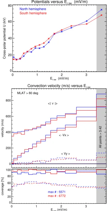
high-est bins. At that end, the averages start to fluctuate about this level. This can be interpreted as an indication for saturation at |ByzIMF|∼>11 nT. Potentials versus Er sw (mV/m) 0 1 2 3 Er sw (mV/m) 0 20 40 60 80 Cross-polar potential U (kV) North hemisphere South hemisphere
Convection velocity (m/s) versus Er,sw
0 200 400 600 800 velocity (m/s) < -Vx > < Vy > All points > 3.42 0 1 2 3 Er,sw (mV/m) 0 20 40 60 80 100 coverage [%] max # : 5571 max # : 6772 MLAT > 80 deg
Fig. 9. Top: Cross-polar cap potentials as function of the solar wind
reconnection electric field, Er,sw, for both North (blue) and South
(red) high-latitude convection pattern, derived for each bin sepa-rately (cf. Paper 1). Here, again we use variable step widths as in Fig. 8. Middle: Central polar cap convection velocities for the same variable bin steps as above, but averaged within the central polar cap at magnetic latitudes at |φm|>80◦only. The bottom panel
shows the coverage characteristics for each bin like in Fig. 7.
4.3 Dependence on solar wind electric field
Figure 9 shows the cross polar cap potential estimations (up-per panel), the average convection velocities h−Vxiand hVyi
(>80◦), and the convection magnitude hV i (middle panel) as function of the solar wind electric field, projected along
Convection velocity (m/s) versus Pdyn 0 200 400 600 velocity (m/s) < -Vx > < Vy > 1 2 3 4 5 Pdyn (nPa) 0 20 40 60 80 100
coverage [%] Both hemispheresMLAT > 80 deg max # : 33768
a
Convection velocity (m/s) versus s.w. proton density
0 200 400 600 velocity (m/s) < -Vx > < Vy > 0 2 4 6 8 10 12 s.w. proton density (cm-3) 0 20 40 60 80 100
coverage [%] Both hemispheresMLAT > 80 deg max # : 27813
b
Convection velocity (m/s) versus V_sw
0 200 400 600 velocity (m/s) < -Vx > < Vy > 350 400 450 500 550 V_sw (km/s) 0 20 40 60 80 100
coverage [%] Both hemispheresMLAT > 80 deg max # : 20744
c
Fig. 10. (a):The polar cap convection velocity shown as function of the solar wind dynamic pressure Pdyn; (b, c): the corresponding
dependencies of the solar wind proton density np and velocity |Vs.w.|. Data points from both hemispheres have been combined for the
analysis. The bottom panels indicate the spatial coverage characteristics for each bin within the high-latitude area (|φm|>80◦).
the dayside reconnection X-line according to the method by Sonnerup (1974):
Er,sw =Eyz,sw sin2(θ/2) = Vx,swByz,swIMF sin2(θ/2) (3)
where Eyz,sw is the solar wind electric field, Vx,swis the
X-component of the solar wind velocity, |ByzIMF|is the interplan-etary magnetic field in the GSM yz-plane, and θ is the IMF clock angle. As seen from Eq. (3), this parameter strongly depends on the direction of the IMF. The electric field Er,sw
serves as an indicator of the reconnection rate at the frontside magnetopause (dayside reconnection), or, for a fixed length of the reconnection line, of the cross-polar cap potential drop. As expected, there is a clear correlation between the an-tisolar convection velocity h−Vxi and Er,sw. Higher
recon-nection rates at the magnetopause cause faster transport of flux across the polar cap. As noted in Paper 1, the convection between the main cells is slow, but still antisunward over the central polar cap, for low values of Er,sw(which typically
dicate a northward directed IMF). Closer inspection of the in-dividually averaged components hVxiand hVyishow, that at
low values of Er,sw the sunward convection, which is taking
place within the lobe cells, and the usual antisunward convec-tion cancel each other within the high-latitude circle at mag-netic latitudes >80◦, so that h−V
xishows the straight linear
behaviour, starting at zero. In contrast, the potential curves have a finite magnitude of ≈15 kV for vanishing Er,swas they
result from the remaining main convection cells. The hVyi
component increases slowly with increasing values of Er,sw,
starting close to zero and raising up to 50–100 m s−1over the range shown in Fig. 9. While there is linear correlation for values of Er,sw(up to almost 2 mV m−1), the curve then
flat-tens out, but does not saturate, as demonstrated by the fact
that the last bin, which collects all Er,sw values above
ap-proximately 3.4 mV m−1, still shows a significant increase. This issue of potential saturation has been addressed by Sis-coe et al. (e.g. 2002); Hairston et al. (e.g. 2005).
4.4 Dependence on solar wind dynamic pressure
As mentioned, due to the nature of statistical studies, we are not able to investigate the direct response to time variances such as pressure pulses or sudden reductions in the dynamic pressure. But we can draw conclusion about the statistical behaviour of a large data set.
Figures 10a–c show the solar wind dynamic pressure Pdyn
(left panel) together with the parameters it is constructed from, namely the solar wind proton density np (middle
panel) and the solar wind velocity |Vs.w.|(right panel). They
are related according to Pdyn=mpnpVs.w.2 , where mp is the
proton mass. No significant North-South asymmetries were found for the convection velocities. Therefore we are com-bining measurements from both hemispheres in this plot. This is done by folding the Southern data points into the Northern by inverting the ByIMFdependence. The bottom pan-els indicate the spatial coverage characteristics for each bin within the high-latitude area (|φm|>80◦).
The drift velocity averages show a weak positive correla-tion with Pdyn (upper panel of Fig. 10a). Even more
inter-estingly, at very low pressures there seems to be a significant peak, that is, low Pdynare related to higher convection
veloc-ities. The reason for this is not clear, but the data coverage is good, so the effect seems to be real and it is related to the solar wind density, which reveals this peak at very low densi-ties (upper panel of Fig. 10b). The further variation with the proton density is quite flat, except of a secondary small peak
Convection velocity (m/s) versus DOY 0 200 400 600 velocity (m/s) < -Vx > < Vy > 100 200 300 DOY (days) 0 20 40 60 80 100
coverage [%] MLAT > 80 deg max # : 9364max # : 17152
a
North hemisphere
South hemisphere
Convection velocity (m/s) versus DOY
0 200 400 600 velocity (m/s) < -Vx > < Vy > 100 200 300 DOY (days) 0 20 40 60 80 100
coverage [%] MLAT > 80 deg max # : 7745max # : 7873
b
North hemisphere
South hemisphere
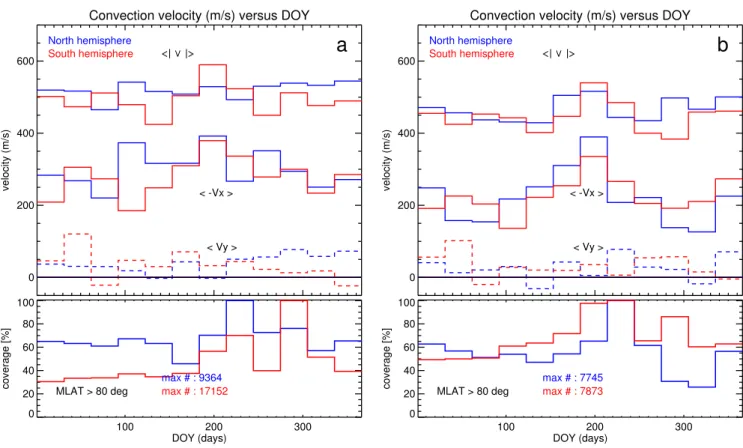
Fig. 11. Average convection velocity variations versus Day of the Year (DOY) (or seasonal dependencies) for the Northern (blue curves) and
Southern Hemisphere (red). Left (a): using all data points of our data set. Right (b): using a filtered data set with Dst>−30 nT only (quiet
conditions). The bottom panels illustrate the data coverage of the 12 equally sized steps corresponding to approximately monthly resolution.
in the range of 7–8 cm−3. The slow rise of the convection ve-locities with increasing Pdynis explained by a corresponding
rise in the solar wind speed, shown in Fig. 10c.
Equating the velocity variations with cross-polar cap po-tential variations, we expect that there should be an increased potential at very low Pdynvalues which is due primarily to a
solar wind density effect. The amplitude of this effect is up to about 25% relative to the level at mean solar wind dynamic pressure.
4.5 Seasonal variations
In Fig. 11 we tried to estimate possible seasonal variations that could be revealed from our data set. Due to the orbital constraints, as explained in Paper 1, Sect. 3.4, only the very central part of the polar cap can be considered as equally cov-ered with data points throughout the whole year, though the mapped drift vectors might originate from different spatial volumes of the magnetosphere.
Several studies in the past investigated the seasonal depen-dencies of the large-scale high-latitude convection pattern, but many studies (e.g., De La Beaujardiere et al., 1991; Rich and Hairston, 1994; Weimer, 1995; Ruohoniemi and Green-wald, 1995; Milan et al., 2001) came to different or even
con-tradictory results. Ruohoniemi and Greenwald (1995, 2005) found that the seasonal effect is similar to that of the sign of ByIMF. They state that the combination of By+/summer
(By–/winter) reinforces the tendency of the ByIMFsign factor
to sculpt the dusk and dawn cells into more round/crescent shapes and to shift the crescent cell across the midnight MLT meridian while lowering the total cross polar cap poten-tials. The non-reinforcing combinations, on the other hand, produce elevated cross-polar potentials, especially for By–
/summer conditions and they found an overall tendency for the cross polar cap potential to increase from winter to sum-mer. These conclusions of the Ruohoniemi and Greenwald (2005) study are based on Northern Hemisphere observations of the SuperDARN network.
The upper pair of curves in the upper panel of Fig. 11a, showing the seasonal variation of the averages of the drift magnitudes, h|V |i, reveal the generally higher level of North-ern Hemisphere velocity. On average, this amounts to about 7% for the whole area of our high-latitude grids, as already mentioned in Sect. 1, and it is slightly smaller but still visible within the 80◦circle shown here. The relative seasonal vari-ations of this parameter are very small, i.e., less than 10% at the Northern Hemisphere and somewhat larger (up to ≈20%)
at the Southern. The weak trend shows slight maxima (if ever) during winter months of the respective Hemisphere. The velocity averages h−Vxiin Fig. 11a show a somewhat
different behaviour. The relative seasonal variations and the variations from month to month are larger and the annual variation seem to be more-or-less in phase with the upper curves in case of the Southern Hemisphere, while it seems to be in opposite phase at the Northern.
After filtering the time series for geomagnetically undis-turbed conditions, as is done in Fig. 11b for Dst>30 nT, a
clear semiannual variation becomes evident with larger con-vection values during solstices for both hemispheres. The July maximum (Northern summer) seems to be more pro-nounced than that of December/January. It is well known that geomagnetic storms are more frequent during the equinoxes. This was discovered by analyzing time series of
geomag-netic indices. The semiannual variation (and to a
mi-nor degree also a diurnal variation) has been explained by the Russell-McPherron (R-M) effect (Russell and McPher-ron, 1973) as being due to the geometrical relationship be-tween the Earth’s dipole axis and the Parker spiral plane. Additionally, the semiannual effect has recently be shown to originate also from the periodical change of the solar wind–magnetosphere–ionosphere (SMI) coupling efficiency (e.g., Cliver et al., 2004; Nagatsuma, 2006) which leads to more frequent and stronger geomagnetic storms near the equinoxes. During quiet-time conditions, on the other hand, we observe on average enhanced and more ordered convec-tion during solstice periods, as shown in Fig. 11b. The rea-son for this is not yet clear, but can probably be related to thermosphere–ionosphere influences on the magnetospheric convection. This should be analyzed in more detail in a fu-ture study.
The relative variations for unfiltered data (Fig. 11a) are generally larger at the Southern Hemisphere. Seasonal vari-ations are likely to be related to different illumination condi-tions (cf. Fig. 2) and therefore different ionospheric conduc-tances. The larger relative variations in the Southern Hemi-sphere might also partially be caused by differences in the ge-omagnetic field configuration. Whereas the Northern Hemi-sphere IGRF field poleward of 58◦ is fairly homogeneous, the Southern Hemisphere contains many crustal anomalies, causing a larger spatial variation in the magnetic field. Values of the IGRF magnetic field at 400 km altitude in the North-ern Hemisphere ≥58◦range from 42.9 to 49.9 µT , with an average of 47.4 µT . For the Southern Hemisphere, the cor-responding spatial variation is between 30.8 to 54.7 µT , with an average of 49.7 µT . Time variations of the IGRF field in the period from February 2001 to March 2006 are slow and insignificant in this connection.
The data coverage, shown in the bottom panel of Fig. 11, is largest around the September equinox for both hemispheres with the Southern maximum being larger than the Northern. During this time of the year, the Cluster satellites have their apogee in the tail magnetosphere and spend relatively long
Convection velocity (m/s) versus Dst
0 200 400 600 800 velocity (m/s) < -Vx > < Vy > 20 0 -20 -40 -60 -80 Dst (nT) 0 20 40 60 80 100 coverage [%] max # : 26744 Both hemispheres MLAT > 80 deg
Fig. 12. Top: Dependence of the average convection velocities on
the Dstindex, with data from both hemispheres combined. Bottom:
number of data points with equally sized steps, in percentage of the maximum indicated.
time intervals there. As mentioned earlier, due to the south-ward tilt of the line of apsides of the Cluster orbit, the satel-lites spend more time below the neutral sheet on the mag-netospheric tailside which maps to the Southern Hemisphere nightside ionosphere.
Generally, the seasonal effect is minor with maximum am-plitudes of 10% to 30% at most in the cross-polar potential as deduced from the locally confined average velocity esti-mations of h−Vxi within the central polar cap. According
to the same reasoning, an overall tendency for a semiannual variation of the cross polar cap potential during geomagneti-cally undisturbed conditions is likely with on average larger potentials during solstices.
4.6 Dependence on the Dst index
Figure 12 shows the correlation with the Disturbed Storm Time (Dst) index. The Dstindex is a measure of the
horizon-tal magnetic deflection on the Earth at equatorial latitudes. Negative deflections in Dst are mainly controlled by Earth’s
ring current, though the solar wind pressure also contributes (e.g., Siscoe et al., 1968; Burton et al., 1975; O’Brien and McPherron, 2000). Positive deflections are usually caused by pressure enhancements in the solar wind which cause a displacement of the magnetospheric drift shells.
Fig. 13. This sketch, taken from Cowley and Lockwood (1992),
il-lustrates the polar cap convection for (a) dayside reconnection not balanced by concurrent nightside reconnection; (b) tail reconnec-tion without concurrent dayside reconnecreconnec-tion. For further details – see Cowley and Lockwood (1992).
Typically, the ring current increases (thus creating a nega-tive deflection of Dst ) during periods of increased cross-tail
electric field, which is typically caused by enhanced dayside reconnection. From this argument, one should therefore ex-pect some degree of correlation with polar cap convection ve-locity. However, processes in the magnetotail, such as bursty bulk flows or substorm activity also influence the Dst index
(e.g., Baumjohann et al., 1996; Friedrich et al., 1999; Baker et al., 2001). Energization is usually very fast, whereas vari-ous loss processes such as charge exchange, pitch angle scat-tering, radial diffusion etc. have much longer time scales (e.g., Cowley, 1977; Daglis et al., 1999).
The clear correlation apparent from Fig. 12 supports the idea that enhanced convection translates into an increase in the cross tail electric field, and thus an energization of the ring current and subsequent negative Dst deflection.
Simi-larly, the higher convection velocity for positive Dst values
may reflect the solar wind pressure pulses and associated dis-placements of magnetospheric drift shells. No North-South asymmetries were found, so the convection velocities are av-erages based on measurements from both hemispheres.
5 Effect of tail magnetic activity
High-latitude plasma convection is not completely deter-mined by dayside coupling, as expressed by the concurrent orientation of the IMF at the magnetopause, but also by processes in the magnetotail that are only indirectly linked to concurrent IMF conditions (e.g., Cowley and Lockwood, 1992) as schematically illustrated in Fig. 13. We demonstrate this point with the EDI potential maps for northward IMF. This is because for strongly northward IMF, no dayside re-connection is expected to occur, and thus the patterns is most sensitive to effects from tail activity.
To enhance the statistical relevance, we use instead of Sec-tor 0 the full “Quadrant 0” of northward directed IMF, i.e. a clock angle range of ±45◦ centered around 0◦, as well
as both hemispheres together (mirroring ByIMFof the South-ern high-latitude data points by sign change). Dividing the Quadrant 0 data according to the level of the ASYM-H index that we have taken as proxy for magnetic activity, and con-structing the corresponding potential maps, as described in Paper 1, we arrive at Fig. 14. The potential maps for low ASYM-H (left panel) and high ASYM-H (right) are con-structed from about equally populated half-distributions (see Fig. 1), below and above an ASYM-H value of 20 nT, respec-tively.
For the dayside, both maps show the lobe cells resulting from lobe reconnection, as expected for strongly northward IMF. But for the nightside, there is a strong difference in the spacing of the iso-potential contours, indicating much stronger convection for high values of ASYM-H. This is ex-actly what is expected from reconnection in the magnetotail associated with high magnetic activity, as shown in Fig. 13.
6 Summary
Based on a data set of more than 5800 h of convection veloc-ity measurements from the Cluster EDI experiment, mapped into the ionosphere, we have investigated the variability as well as the solar wind and IMF dependencies of the high-latitude convection.
– The variability of the high-latitude convection shows, similar to the convection itself, characteristic spatial patterns of dependence of the ByIMFcomponent which
Fig. 14. Potential patterns for northward IMF and two levels of nighside activity. Left: Low values of ASYM-H <20 nT, indicating little or
no auroral activity. Right: High ASYM-H values (≥20 nT), indicating strong partial ring current activity. The full Quadrant 0 of clock angle distribution, i.e. ±45◦centered around 0◦, and North and South Hemisphere combined have been used to derive the potential maps.
are mirror symmetric between the Northern and South-ern Hemispheres. The variances (standard deviations) are of the same order as or even larger than the convec-tion magnitude within the auroral oval in particular. – The average convection velocity in XSM direction (i.e.,
the dawn-dusk electric field strength) within the central part of the polar cap (>80◦) can be used alternatively to the cross-polar cap potential for the study of magneto-spheric forcings and their dependencies on various solar wind and IMF parameters. It shows very similar varia-tions, but represents rather solar wind-magnetosphere coupling conditions at mostly ’open’ flux tubes within the central polar cap.
– Correlation with external drivers such as the solar wind dynamic pressure and IMF magnitude in the GSM y-z plane, |ByzIMF|, are in agreement with earlier results (Papitashvili and Rich, 2002; Ruohoniemi and Green-wald, 2005; Matsui et al., 2005). The qualitative be-haviour with positive correlations between the velocity (and thus potential) and these drivers are also repro-duced by model calculations (e.g., Weimer, 2001). – Except for purely northward directed IMF, there is a
clear correlation between the IMF magnitude, |ByzIMF|, and convection velocities. Our data set contains a larger proportion sunlit observations from the Southern Hemi-sphere. Average convection velocities there are system-atically somewhat lower than Northern Hemisphere
val-ues. A positive correlation also exist between |ByzIMF| and the polar cap potential, but no North-South asym-metry was found in the absolute values of the potentials. – Low to moderate values of the solar wind electric field are positively correlated with the convection velocity. For values of Er,swabove approximately 2 mV m−1the
potential does not rise linearly with Er,sw, but seems to
flatten out.
– A positive correlation is found between convection ve-locity and solar wind dynamic pressure Pdyn , but
ad-ditionally there appears an enhanced convection speed (cross polar cap potential) for very low values of Pdyn.
This latter peak is due to solar wind density effects, the reason for which are not yet clear.
– Seasonal variations are found to be of minor impor-tance (of the order of 10% to 30%). They are more pronounced and show a clear semiannual variation with maxima of convection during solstices for geomagneti-cally quiet periods only.
– There is a positive correlation between ring current en-ergization (reflected by the Dst index) and the
convec-tion velocity. This demonstrates that a part of the ring current is directly driven by enhanced dayside recon-nection.
– We also find a positive correlation between nighside activity/processes in the magnetotail (reflected by the
ASYM-H index) and convection velocity. A large ASYM-H index corresponds to higher polar cap poten-tial.
Since our data set is not continuous in time, we are unable to address statistical time dependencies such as response times or decay times. Such studies will have to be based on shorter, continuous time segments in the data set. This will be ad-dressed in future publications.
Acknowledgements. Work at GeoForschungsZentrum (GFZ)
Pots-dam was supported by Deutsche Forschungsgemeinschaft (DFG). Work at the Max-Planck- Institut f¨ur extraterrestrische Physik was supported by Deutsches Zentrum f¨ur Luft- und Raumfahrt (DLR). Research at the University of Bergen was supported by the Norwe-gian Research Council. Work by U.S. investigators was supported in part by NASA grant NNG04GA46G. Parts of the data analysis were done with the QSAS science analysis system provided by the UK Cluster Science Centre (Imperial College London and Queen Mary, University of London) supported by PPARC UK. We thank the ACE SWEPAM and MAG instrument teams and the ACE Sci-ence Center for providing the ACE data, and the World Data Center for Geomagnetism, Kyoto, for providing the Dst and ASYM-H
in-dices. We thank M. Chutter for his support of EDI data analysis and processing, and G. Leistner for providing the averaged EDI data.
Topical Editor I. A. Daglis thanks two anonymous referees for their help in evaluating this paper.
References
Axford, W. I. and Hines, C. O.: A unifying theory of high-latitude geophysical phenomena and geomagnetic storms, Can. J. Phys., 39, 1433–1464, 1961.
Baker, D. N., Turner, N. E., and Pulkkinen, T. I.: Energy transport and dissipation in the magnetosphere during geomag-netic storms, J. Atmos. Terr. Phys., 63, 421–429, doi:10.1016/ S1364-6826(00)00169-3, 2001.
Banks, P. M.: Magnetospheric processes and the behavior of the neutral atmosphere, Space Res., 12, 1051–1067, 1972.
Baumjohann, W., Kamide, Y., and Nakamura, R.: Storms, sub-storms and the near-Earth tail, J. Geomag. Geoelectr., 48, 177– 185, 1996.
Boyle, C. B., Reiff, P. H., and Hairston, M. R.: Empirical polar cap potentials, J. Geophys. Res., 102, 111–125, 1997.
Bristow, W. A., Greenwald, R. A., Shepherd, S. G., and Hughes, J. M.: On the observed variability of the crosspolar cap potential, J. Geophys. Res., 109, A02203, doi:10.1029/2003JA010206, 2004.
Burke, W. J., Kelley, M. C., Sagalyn, R. C., Smiddy, M., and Lai, S. T.: Polar cap electric field structures with a northward inter-planetary magnetic field, Geophys. Res. Lett., 6, 21–24, 1979. Burton, R. K., McPherron, R. L., and Russell, C. T.: An empirical
relationship between interplanetary conditions and Dst, J. Geo-phys. Res., 80, 4204–4214, 1975.
Cliver, E. W., Svalgaard, L., and Ling, A. G.: Origins of the semi-annual variation of geomagnetic activity in 1954 and 1996, Ann. Geophys., 22, 93–100, 2004,
http://www.ann-geophys.net/22/93/2004/.
Codrescu, M. V., Fuller-Rowell, T. J., and Foster, J. C.: On the importance of E–field variability for Joule heating in the high-latitude thermosphere, Geophys. Res. Lett., 22, 2393–2396, 1995.
Codrescu, M. V., Fuller-Rowell, T. J., Foster, J. C., Holt, J. M., and Cariglia, S. J.: Electric field variability associated with the Millstone Hill electric field model, J. Geophys. Res., 105, 5265– 5274, 2000.
Cole, K. D.: Damping of magnetospheric motions by the iono-sphere, J. Geophys. Res., 68, 3231–3235, 1963.
Coroniti, F. V. and Kennel, C. F.: Can the ionosphere regulate mag-netospheric convection?, J. Geophys. Res., 78, 2837–2851, 1973. Cowley, S. W. H.: Pitch angle dependence of the charge-exchange lifetime of ring current ions, Planet. Space Sci., 25, 385–393, doi:10.1016/0032-0633(77)90054-X, 1977.
Cowley, S. W. H. and Lockwood, M.: Excitation and decay of so-lar wind-driven flows in the magnetosphere-ionosphere system, Ann. Geophys., 10, 103–115, 1992,
http://www.ann-geophys.net/10/103/1992/.
Crowley, G. and Hackert, C. L.: Quantification of High Latitude Electric Field Variability, Geophys. Res. Lett., 28, 2783–2786, 2001.
Daglis, I. A., Thorne, R. M., Baumjohann, W., and Orsini, S.: The terrestrial ring current: Origin, formation, and decay, Rev. Geo-phys., 37, 407–438, 1999.
De La Beaujardiere, O., Alcayde, D., Fontanari, J., and Leger, C.: Seasonal dependence of high-latitude electric fields, J. Geophys. Res., 96, 5723–5735, 1991.
Dungey, J. W.: Interplanetary magnetic field and the auroral zones, Phys. Rev. Lett., 6, 47–48, 1961.
Friedrich, E., Rostoker, G., Connors, M. G., and McPherron, R. L.: Influence of the substorm current wedge on the Dst index, J. Geo-phys. Res., 104, 4567–4576, 1999.
Haaland, S. E., Paschmann, G., F¨orster, M., Quinn, J. M., Torbert, R. B., McIlwain, C. E., Vaith, H., Puhl-Quinn, P. A., and Klet-zing, C. A.: High-latitude plasma convection from Cluster EDI measurements: Method and IMF-dependence, Ann. Geophys., 25, 239–253, 2007,
http://www.ann-geophys.net/25/239/2007/.
Hairston, M. R., Drake, K. A., and Skoug, R.: Saturation of the ionospheric polar cap potential during the October–November 2003 superstorms, J. Geophys. Res., 110, A09S26, doi:10.1029/ 2004JA010864, 2005.
Heppner, J. P. and Maynard, N. C.: Empirical high–latitude electric field models, J. Geophys. Res., 92, 4467–4489, 1987.
Hill, T. W.: Mercury and Mars: The role of ionospheric conductivity in the acceleration of magnetospheric particles, Geophys. Res. Lett., 3, 429–432, 1976.
Matsui, H., Quinn, J. M., Torbert, R. B., Jordanova, V. K., Puhl-Quinn, P. A., and Paschmann, G.: IMF BY and the seasonal de-pendences of the electric field in the inner magnetosphere, Ann. Geophys., 23, 2671–2678, 2005,
http://www.ann-geophys.net/23/2671/2005/.
Milan, S. E., Baddeley, L. J., Lester, M., and Sato, N.: A seasonal variation in the convection response to IMF orientation, Geo-phys. Res. Lett., 28, 471–474, 2001.
Nagatsuma, T.: Diurnal, semiannual, and solar cycle variations of solar windmagnetosphereionosphere coupling, J. Geophys. Res., 111, A09202, doi:10.1029/2005JA011122, 2006.
O’Brien, T. P. and McPherron, R. L.: An empirical phase space analysis of ring current dynamics: Solar wind control of injec-tion and decay, J. Geophys. Res., 105, 7707–7719, doi:10.1029/ 1998JA000437, 2000.
Papitashvili, V. O. and Rich, F. J.: High-latitude ionospheric con-vection models derived from Defense Meteorological Satellite Program ion drift observations and parameterized by the inter-planetary magnetic field strength and direction, J. Geophys. Res., 107, 1198, doi:10.1029/2001JA000264, 2002.
Reiff, P. H. and Burch, J. L.: IMF By-dependent plasma flow and Birkeland currents in the dayside magnetosphere, 2. A global model for northward and southward IMF, J. Geophys. Res., 90, 1595–1609, 1985.
Reiff, P. H. and Heelis, R. A.: Four cells or two? Are four convec-tion cells really necessary?, J. Geophys. Res., 99, 3955–3960, 1994.
Reiff, P. H., Spiro, R. W., and Hill, T. W.: Dependence of polar cap potential drop on interplanetary parameters, J. Geophys. Res., 86, 7639–7648, 1981.
Rich, F. J. and Hairston, M. R.: Large-scale convection patterns observed by DMSP, J. Geophys. Res., 99, 3827–3844, 1994. Rostoker, G., Savoie, D., and Phan, T. D.: Response of
magnetosphere-ionosphere current systems to changes in the in-terplanetary magnetic field, J. Geophys. Res., 93, 8633–8641, 1988.
Ruohoniemi, J. M. and Greenwald, R. A.: Observations of IMF and seasonal effects in high-latitude convection, Geophys. Res. Lett., 9, 1121–1124, 1995.
Ruohoniemi, J. M. and Greenwald, R. A.: Dependencies of high-latitude plasma convection: Consideration of interplane-tary magnetic field, seasonal, and universal time factors in sta-tistical patterns, J. Geophys. Res., 110, A09204, doi:10.1029/ 2004JA010815, 2005.
Russell, C. T. and McPherron, R. L.: The magnetotail and sub-storms, Space Sci. Rev., 15, 205–266, 1973.
Siscoe, G. L., Formisano, V., and Lazarus, A. J.: Relation between geomagnetic Sudden Impulses and solar wind pressure changes – An experimental investigation, J. Geophys. Res., 73, 4869–4874, 1968.
Siscoe, G. L., Crooker, N. U., and Siebert, K. D.: Transpolar po-tential saturation: Roles of region 1 current system and solar wind ram pressure, J. Geophys. Res., 107, 1321, doi:10.1029/ 2001JA009176, 2002.
Sonnerup, B. U. ¨O.: Magnetopause reconnection rate, J. Geophys. Res., 79, 1546–1549, 1974.
Tanaka, T.: Interplanetary magnetic field By and auroral conduc-tance effects on high-latitude ionospheric convection patterns, J. Geophys. Res., 106, 24 505–24 516, 2001.
Weimer, D. R.: Models of high latitude electric potentials derived with a least error fit of spherical harmonic coefficients, J. Geo-phys. Res., 100, 19 595–19 607, 1995.
Weimer, D. R.: An improved model of ionospheric electric po-tentials including substorm perturbations and application to the Geospace Environment Modeling November 24, 1996, event, J. Geophys. Res., 106, 407–416, 2001.

![Fig. 5. Standard deviation of the total vector variation [m s −1 ] of EDI drift vectors mapped to the Northern high latitude ionosphere for the time interval from Feb 2001 to Mar 2006](https://thumb-eu.123doks.com/thumbv2/123doknet/14800500.605982/8.892.152.749.92.695/standard-deviation-variation-vectors-northern-latitude-ionosphere-interval.webp)