Empirical Assessment of Multimorphic Testing

RESEARCH OUTPUTS / RÉSULTATS DE RECHERCHE

Author(s) - Auteur(s) :

Publication date - Date de publication :

Permanent link - Permalien :

Rights / License - Licence de droit d’auteur :

Bibliothèque Universitaire Moretus Plantin

Institutional Repository - Research Portal

Dépôt Institutionnel - Portail de la Recherche

researchportal.unamur.be

University of Namur

Empirical Assessment of Multimorphic Testing

Temple, Paul; Acher, Mathieu; Jézéquel, Jean-Marc

Published in:

IEEE Transactions on Software Engineering

Publication date:

2019

Link to publication

Citation for pulished version (HARVARD):

Temple, P, Acher, M & Jézéquel, J-M 2019, 'Empirical Assessment of Multimorphic Testing', IEEE Transactions

on Software Engineering.

General rights

Copyright and moral rights for the publications made accessible in the public portal are retained by the authors and/or other copyright owners and it is a condition of accessing publications that users recognise and abide by the legal requirements associated with these rights. • Users may download and print one copy of any publication from the public portal for the purpose of private study or research. • You may not further distribute the material or use it for any profit-making activity or commercial gain

• You may freely distribute the URL identifying the publication in the public portal ? Take down policy

If you believe that this document breaches copyright please contact us providing details, and we will remove access to the work immediately and investigate your claim.

1

Empirical Assessment

of Multimorphic Testing

Paul Temple, Mathieu Acher and Jean-Marc Jézéquel

F

Abstract—The performance of software systems such as speed, memory usage, correct identification rate, tends to be an evermore important concern, often nowadays on par with functional correctness for critical systems. Systemat-ically testing these performance concerns is however ex-tremely difficult, in particular because there exists no theory underpinning the evaluation of a performance test suite, i.e., to tell the software developer whether such a test suite is "good enough" or even whether a test suite is better than another one. This paper proposes to apply Multimorphic testing and empirically assess the effectiveness of perfor-mance test suites of software systems coming from various domains. By analogy with mutation testing, our core idea is to leverage the typical configurability of these systems, and to check whether it makes any difference in the outcome of the tests: i.e., are some tests able to “kill” underperform-ing system configurations? More precisely, we propose a framework for defining and evaluating the coverage of a test suite with respect to a quantitative property of interest. Such properties can be the execution time, the memory usage or the success rate in tasks performed by a software system. This framework can be used to assess whether a new test case is worth adding to a test suite or to select an optimal test suite with respect to a property of interest. We evaluate several aspects of our proposal through 3 empir-ical studies carried out in different fields: object tracking in videos, object recognition in images, and code generators.

Index Terms—software product lines; software testing; performance testing; test evaluation

1

I

On May 7, 2016, a 2015 Tesla Model S collided with a tractor trailer crossing an uncontrolled intersection on a highway west of Williston, Florida, USA, resulting in fatal injuries to the Tesla driver. On January 19, 2017, the NHTSA (National Highway Traffic Safety Administra-tion) released a report on the investigation of the safety of the Tesla autonomous vehicle control system. Data obtained from the Model S indi-cated that: 1) the Tesla was being operated in

P. Temple is now with the PReCISE, NaDi, Unamur. Email: paul.temple@unamur.be

M. Acher and J.M. Jézéquel are with the Univ Rennes, IRISA, Inria, CNRS.

EMail: firstname.lastname@irisa.fr

Autopilot mode at the time of the collision; 2) the Automatic Emergency Braking (AEB) system did not provide any warning or automated braking for the collision event; and 3) the driver took no braking, steering or other actions to avoid the col-lision. The conclusion was the investigation did not reveal any safety-related defect with respect to predefined requirements from the system. However, the crash did actually occur. Without questioning the legal aspects that are definitively covered in the NHTSA report, one might wonder why the computer vision program did not “see” this huge trailer in the middle of the road. Of course, a posteriori, it is easy to understand that the Tesla crash videos recorded by Autopilot were not under ideal lighting conditions. Back-ground objects blended into vehicles that needed to be recognized, making it difficult for any com-puter to process the video stream correctly. On top of that, no wheels were visible under the trailer, which complicated its identification as a vehicle in the middle of the road. More recently, on March 18, 2018, an autonomous Uber vehicle hit a pedestrian crossing a road in Arizona, USA. The pedestrian crossed outside any near cross-walks, at night, on a road where there were no public lighting. A video of the accident was re-leased a few weeks later showing that the vehicle did not even try to dodge or brake before it hits the person and provokes her death. However, the associated released report stated that the system actually recognized the pedestrian just before the accident, showing that the embedded recognition system did not fail per se but was "only" slow to recognize the pedestrian under such conditions. Now taking a software engineering perspective, these situations clearly lead to the usual question from the software testing community: how come that those systems were deployed without being tested under such conditions? This is, of course, partly due to a huge input data space. Going further, since the input space (e.g., videos for testing video tracking) is orders of magnitude larger than typical data, we ask the following set of questions: how much effort should we put in

the testing activity? How can we build a “good” test suite? How do we even know that a given test suite is “better” than another one? Structural code coverage metrics for test suites seem indeed a bit shaky for that kind of software systems, especially for handling quantitative properties re-lated to performance aspects. This general prob-lem does not only apply to Computer Vision systems. For instance, Generative Programming techniques have become a common practice in software development to deal with the hetero-geneity of platforms and technological stacks that exist in several domains such as mobile or In-ternet of Things. Generative programming offers a software abstraction layer that software devel-opers can use to specify the desired system’s behavior and automatically generate software ar-tifacts on different platforms. As a consequence, multiple code generators (also called compilers) are used to transform the specifications/models represented in graphical or textual languages into different general-purpose programming lan-guages such as C, Java, C++, etc. or different byte code or machine code. In this case, from a testing point of view, the input data space is made of models or programs. Defective code generators with respect to performance speed, memory usage, correct identification rate, such as high resource usage or low execution speed, are then hard to detect since testers need to produce and interpret numerous numerical results.

In this paper, we empirically assess the Multi-morphic Testing approach which has been briefly introduced in [1], as a method for estimating the relative strength of performance test suites, using a new metric that we call the dispersion score. By analogy with mutation testing, our core idea is to check whether testing different variants imple-menting the same functionality yields significant differences on the outcome of the tests. These variants are called morphs hereafter. Contrary to functional testing where a clear pass/fail verdict can be used to kill mutants and get a mutation score for the test suite, performance testing can only show performance differences among a set of morphs. With the intuition that a good test suite should be able to highlight outliers among these morphs, we introduce the notion of disper-sion score of a test suite to characterize its ability to differentiate morphs of the same system. This work focuses on performance testing and, as such, Multimorphic testing should typically be used after "traditional" functional testing tech-niques.

Organization of the paper.Section2presents

our method including the definition of our dis-persion score. To show its applicability to vari-ous domains, we validate our approach on three different applications in Section 3 (i.e., video tracking, image recognition and code generators).

Section 4discusses some threats of our method and evaluation process. Section5presents related work before concluding and proposing future investigation axis in Section6.

2

M

T

2.1 Motivation

While functional tests use an Oracle that gives a "pass"/"fail" verdict to check the output confor-mance of a program, perforconfor-mance testing aims to assess quantitative properties through the execu-tion of software under various condiexecu-tions. This assessment can be confronted to user-defined requirements, such as "I need a system that is able to process inputs under a fixed amount of time". In the end, the characterization and confrontation process can provide level of insurances about performances of a system. For instance, "From the test I ran, I saw that the system was able to process inputs under 30 seconds in 7 out of 10 cases". One crucial aspect of this process is that the assessment of performances heavily depends on test cases (or given inputs) fed to software systems.

Example 1. For instance, let us consider a

Computer Vision (CV) based system designed to detect objects. A key performance indicator could be its precision, defined as the ratio of correctly identified objects with respect to ground truth. Getting a low precision on a given test case (e.g., an image) does not necessarily mean the test case is good and that the CV program is weak, because the test case might simply be too difficult (e.g., a scene with low contrast and poor illumina-tion condiillumina-tions resulting in objects being barely perceivable). Conversely, if the precision is high, does it mean that the computer vision program is efficient or that the video is simply not very challenging (e.g., just one big, highly contrasted object under ideal illumination conditions)?

Example 2.Let us consider another

engineer-ing context. The discovery of (performance) bugs in generators or compilers can be complex. In such a context, what are the most useful test cases considering a test suite that need to be ran in order to find that a generated program using a particular programming language has performance issues such as unexpected high ex-ecution time? Once again, we can understand that very simplistic test cases are not interesting as computation times might be too short: taking milliseconds to execute. Conversely, executing unrealistic test cases may result in extremely long execution time or time-out. Here again, we see that what matters is the fact that we are able to discriminate the execution of different programs. Our general observation is that we cannot assess the performance of a software system solely based on raw and absolute numbers; the

3

performance should rather be put into perspective w.r.t. the difficulty of the task. For doing so, we consider two main axes. First, a software system should be confronted to other morphs in order to establish the relative difficulty of a task. Second, the quality of a test case, and by extension test suites, is crucial. A bad test suite may not reveal the underlying difficulty in processing a certain task1_{. We consider a good test case as one being able}

to discriminate different program implementations based on their observed performances. Overall, we aim to characterize the quality of test suites when assessing quantitative properties of a software system.

2.2 The principle of Multimorphic Testing

In this section, we describe how we can associate a score to a performance test suite2_{, based on its}

ability to discriminate the performance behavior of morphs of the same software system.

The core idea of Multimorphic testing [1] is to evaluate test suites with respect to different morphs being different implementations of the same high-level functionality that should exhibit performance differences. Morphs typically corre-spond to different parameterizations of a system or to different implementation choices that can be selected at compile time or runtime. For instance, using a specific algorithm for video tracking; or using a particular strategy for a compiler. In these cases, Software Product Line automatic deriva-tion techniques [2], [3] can be used to generate a large number of morphs based on the system variability model.

Said differently and by analogy with mu-tation testing: Are good test suites able to “kill” weak morphs? Our basic assumption is that a test is “good” when it is able to reveal signifi-cant quantitative differences in the performances of morphs. Following the same process as for mutation testing, we derive and exploit morphs (instead of mutants) to reveal significant perfor-mance differences (instead of pass/fail verdicts) and eventually assess the relative qualities of test suites.

Our method, called Multimorphic testing, proactively produces morphs that are all tested with the same set of test cases considered as a test suite.

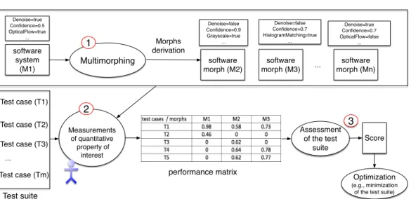
In the example of Figure1, morphs denoted M1, M2, M3, ..., Mn are derived thanks to the

settings of parameters’ values. For instance, in the case of computer vision systems, all morphs

1. from our point of view, these tests are pointless but it does not mean that they should be considered as such in the context of functional testing. On the contrary, some of these "bad" tests can be very useful to detect functional bugs.

2. The score of a single test case is then defined as the score of the singleton test suite made of it.

implement the same high-level functionality and realize the same task, namely tracking objects in a scene. We use different values for parameters such as Denoise, Confidence, or OpticalFlow, be-cause these can have a significant influence on performance properties such as execution time or precision. Once morphs are derived, they can be fed with inputs. Inputs are represented by test cases on the left part of Figure 1. Morphs’ performances (e.g., execution time) are measured for each pair (Mi,Ti). We represented examples

of performances in cells of the performance ma-trix of Figure 1. We remind that those morphs are supposed to be functionally tested and we suppose they are able to perform the high-level functionality they were designed for.

Ultimately, we need a performance measure (or score) that reflects the ability of a test suite to exhibit different performance behaviors among a set of morphs of the same software system.

2.3 Desired Properties of the measure

We want the performance measure to have the following properties:

• (P1) non-negativity: the measure associ-ated to a test suite should be ≥ 0

• (P2) null empty set: the measure

associ-ated with an empty test suite is 0

• (P3) measure of subsets: considering 2 test suites A and B, if A ⊆ B, then measure(A) ≤ measure(B)

• (P4) measure of test suites:

considering n test suites A1, ...,

An, measure(A1 ∪ ... ∪ An) ≥

max(measure(A1), ..., measure(An)

While P1 and P2 are rather general descriptive behaviors, P3 and P4 are more specific to our case in particular regarding the behavior of the score when evaluated on association/combinations of test suites. P3 states that if a test suite is included in a larger one, the measure associated to the larger test suite cannot be lower than the measure associated to the first test suite. P4 states that the combination of two or more test suites should not have an associated measure lower than the max-imum measure associated to the individual test suites composing the combination of test suites. These two properties stipulate that increasing the size of a test suite should not decrease its associated score.

2.4 Design of dispersion measures

The previous properties aim to restrict the design space of candidate measures and in turn elimi-nate some of them. For example, in this section, we demonstrate that variance, an intuitive and widely used measure, cannot be chosen in our context. We then propose a new measure that we call the dispersion score which does fulfill the wanted properties.

Test suite software system (M1) Denoise=true Confidence=0.5 OpticalFlow=true ... Denoise=false Confidence=0.7 HistogramMatching=true ... Denoise=false Confidence=0.9 Grayscale=true ... software morph (M2) Multimorphing software morph (M3) software morph (Mn) ... Denoise=true Confidence=0.7 OpticalFlow=false ... Measurements of quantitative property of interest Morphs derivation Test case (T1) Test case (T2) Test case (T3) Test case (Tm) ... Assessment of the test suite Optimization (e.g., minimization of the test suite)

Score

2 1

3

performance matrix

Figure 1: Multimorphic process: morphs are automatically produced (e.g., playing with parameters); for each morph the test suite is executed and performance measurements are gathered; a dispersion score is finally computed to characterize the quality of a test suite

2.4.1 Variance

Variance is probably the most commonly used indicator when analyzing the spreading of mea-sures. It computes the difference between ele-ments of a set with the mean value of this set and average these differences to produce a value. It is usually described as: V (X) = Eh(X − E [X])2i with X, a set of observations over a random variable and E, the expected value.

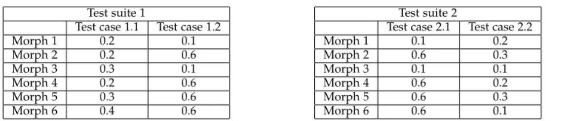
Variance could be interesting but it does not meet the last of our desired properties ((P4) from Section2.3). We give a counterexample in Table1: combining two test suites may actually reduce the variance of the resulting test suite. Specifically, Table 1 shows two test suites (Test suite 1 and Test suite 2) both composed of two test cases. Six Morphs are executed on each test suite. Each execution yields a value in the range [0.1; 0.6].

Let us compute variances of Table1:

• The variance of Test suite 1 is 0.041;

• The variance of Test suite 2 is 0.049;

• The variance of Test suite 1 and 2 is 0.043.

The variance of the combination of the two test suites lies in between the two variances of individual test suite. This counterexample shows that (P3) and (P4) are not always met and thus variance cannot be used in our context.

2.4.2 Dispersion score

Instead, we propose to use a dispersion score that is inspired from histograms, as they are one of the most popular ways of evaluating the distribution of a continuous variable [4], [5]. An example of histogram based on values given by Test suite 1 of Table1is shown in Figure2.

The observed definition domain (i.e., the range of observed values) is presented on the

Figure 2: An example of a histogram (based on Table1).

X-axis, while frequency of observations appears on the Y-axis and is defined between 0 and 1. From left to right, it reads as follows: 16, 5% of observed values lie in the range [0; 0.12], 25% of observed values lie in the range [0.12; 0.24] ... and finally 33% lie in the range [0.48; 0.6].

However, we are not interested in the fre-quency of each value nor in absolute values but rather in the fact that at least one observation falls into each sub-range (called bin) of the X-axis. We consider a representation that is similar to an histogram since the X-axis defines the definition domain. It is also divided into bins since we want to highlight significant performance differences. The Y-axis however now is just a Boolean value indicating whether at least one performance mea-sure falls into that particular bin. Since we want to "cover" the definition domain, the representa-tion associated to a test suite has to be as dense as possible.

5

Test suite 1

Test case 1.1 Test case 1.2 Morph 1 0.2 0.1 Morph 2 0.2 0.6 Morph 3 0.3 0.1 Morph 4 0.2 0.6 Morph 5 0.3 0.6 Morph 6 0.4 0.6 Test suite 2

Test case 2.1 Test case 2.2 Morph 1 0.1 0.2 Morph 2 0.6 0.3 Morph 3 0.1 0.1 Morph 4 0.6 0.2 Morph 5 0.6 0.3 Morph 6 0.6 0.1

Table 1: An example for showing the inadequacy of variance and illustrating our measure: perfor-mance observations gathered for 2 different test suites, each composed of 2 test cases over 6 morphs.

Histograms are parameterized by their num-ber of bins. Bins are defined to gather val-ues which are close from each other (i.e., with insignificant differences). Considering a small number of bins would yield a coarse histogram, gathering values with significant differences. On the other hand, too many bins would yield a very fine-grained histogram, providing more details but likely to separate observations with insignif-icant differences. As a trade-off, we choose to fix the number of bins as the number of morphs to execute3_{. We then define the dispersion score of a}

test suite as the proportion of activated bins (i.e., non empty bins) in its histogram.

To make this definition more precise, let us consider n morphs and a test suite made of m test cases.

Executing the m test cases on the n morphs yields a matrix M with m rows and n columns where each cell Mij holds the measured

perfor-mance value such as precision, recall or execution time, as illustrated in Table1.

When considering performance properties, it may be difficult to compare different sets of executions: one test might take a few seconds while others could take minutes or more. We thus need to apply a normalization step over these observations. That is, we consider the extrema of observed performances and, for each perfor-mance, we apply the following transformation:

x−min

max−min where x is an observed performance,

min and max are respectively the minimal and maximal observed performance of a test suite. After this normalization, all performance values Mij are in the range [0; 1].

Now, we have to compute the representation, inspired from histogram, for M. The result is a vector V of size n (since we decided to set the number of bins to the number of morphs) in which each element Vi represents whether

the corresponding bin is activated or not, i.e. at least one measure Mij falls into it. To do so, we

consider the algorithm1:

The target bin for Mij is the immediate

inte-ger larinte-ger than Mij×n (function ceil()), which we

3. We admit this choice is rather arbitrary, but empirical assessment already shows interesting results with that choice (Section3). In fact, finding the best number of bins is a well-known issue [6]. Finding the optimum in our context remains an open question.

Algorithm 1 the procedure used to build the

representation of a test suite leading to the com-putation of its dispersion score.

(1) let V be a vector of size n filled with 0s;

for all i ∈ 1..n do for all j ∈ 1..m do

(2) let idx = ceil(Mij× n);

(3) set Vidxto 1;

end for end for

set to 1.

After this step, the vector only contains 0s and 1s and the dispersion score is:

Pn

i=1Vi

n

This way, the best possible test suite would activate all the bins of its histogram. That is exactly one observation falls into each bin and yields a dispersion score of 1, meaning it is able to discriminate every morph.

The worst test suite would have a score close to 0 (exactly 1/#morphs), because all morphs would behave the same, thus filling only one bin. Dispersion score is thus defined in [0; 1] satisfying the first desired property defined in Section2.3.

The dispersion score of an empty set (i.e., when no test suites are given) is 0 which satisfies the second property. When trying to combine test suites, the fact that we only care about activated bins to compute dispersion scores ensures that P3 and P4 are satisfied.

3

E

E

We have introduced the Dispersion Score as a new measure to assess the relative merits of perfor-mance test suites. In the following, we want to empirically show that this measure is right, and that it is a right measure.

3.1 Research questions

Is the measure right? To be right, the

Dis-persion Score must at least yield different scores for different test suites, i.e., reflect their ability to exhibit varying performances among of a set of morphs.

We also expect sufficient stability w.r.t. the exact set of morphs used for the measure; so we evaluate the stability of the dispersion score via a sensitivity analysis. Finally, we propose an analysis of the evolution of the dispersion score with respect to the choice of number of bins.

Is it a right measure? Here, we want to

as-sess the correlation between the actual (relative) effectiveness of performance test suites and their dispersion scores. Depending on the domain, this question will take several very different forms, from helping to select test cases able to reveal per-formance bugs in code generators, to reducing a test suite without loosing its ranking capabilities.

3.2 Evaluation settings

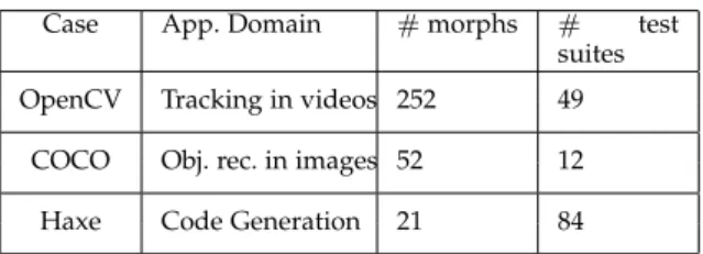
To answer these questions, we applied our method on several application domains and eval-uate its results. For each case, we detail: i) what are morphs; ii) what are test suites; iii) how per-formance measurements are retrieved and used; iv) how we perform the evaluation. Table2 sum-marizes the cases; we can notice different scales both in terms of available morphs and test suites.

Case App. Domain #morphs # test suites OpenCV Tracking in videos 252 49

COCO Obj. rec. in images 52 12 Haxe Code Generation 21 84

Table 2: The three case studies

3.2.1 OpenCV case (object tracking in videos) In the field of video tracking, the use of large test suites helps building confidence in the robustness of a system and its capability in performing well under various conditions. However, are all those test suites necessary? We consider OpenCV4_{, a}

popular library, written in C++, implementing different techniques for tracking object of interest in videos.

Morphs. By reverse-engineering a part of

OpenCV and using the feature modeling formal-ism [7], [3], [2], [8], we have elaborated a vari-ability model (including constraints) to formally specify the possible values of parameters and their valid combinations. From this variability model, we automatically sampled 212 configura-tions by assigning random values to funcconfigura-tions’ parameters. The configurations are valid w.r.t. the variability model and are used to derive 212 morphs.

Test suites.We use a set of 49 synthetic video

sequences. Each video is considered as a test suite on its own composed of only one test case: the

4.https://opencv.org/

video playing the role of the test input data and its ground truth playing the role of the oracle. Videos have been obtained using an industrial video generator [9], [10]. Videos are all different either in the composition of the scene (presence or not of objects we do not want to track such as tree leaves) or in the visual characteristics of the scene (different illumination conditions; presence of heat haze and/or noise). Importantly, a ground truth is automatically generated along videos stating the position of every encrusted objects in every video images such that we can assess the ability of our programs to track objects of interest.

Measurements. Following the Multimorphic

method (see Figure1), we execute all 212 morphs on the 49 videos. For each execution, we measure several quantitative properties such as: Precision, Recall, the execution time and the CPU consumption to cite a few. Precision and Recall measures are ratios given in the range [0; 1]. They are mea-sured by comparing objects’ positions computed by morphs to the generated ground truth. Posi-tions are usually defined by bounding boxes that surround objects. Then, we considered an object as being detected if the intersection between the bounding boxes retrieved by a morph and the one defined by the ground truth is not empty. The execution time is given in seconds while the CPU consumption is expressed as a percentage of one CPU core usage (if the computations are distributed over multiple CPUs then this mea-sure can be higher than 100%). Note that to stay within realistic computation boundaries, we set a time-out for every execution we have launched. If an execution exceed this amount of time, its process is killed and its measures are reported as values showing that it has failed (high CPU and memory consumption, zero Precision and Recall measures, etc.). We have considered 13 different quantitative properties for each execution. This yields a total of 212 ∗ 49 ∗ 13 = 135, 044 perfor-mance measures.

Evaluation.Since our method yields a

disper-sion score associated to a test suite, we evaluate that a test suite created to maximize the disper-sion score is actually a "better" test suite than random ones with lesser scores.

3.2.2 COCO case (object recognition bench-marks)

For many years, the computer vision (CV) com-munity has been building large datasets that are used as benchmarks [11], [12], [13], [14] in com-petitions to rank competing image recognition techniques. Here we use the Microsoft COCO dataset on which CV competitions are conducted every year since 2014. Results of competitions are presented on the leaderboard webpage5_{. COCO}

7

competitions address different tasks such as de-tection of objects or segmentation of images. Our evaluation focuses on object detection.

Morphs.Even if we do not know much about

the specific details of techniques used by com-petitors, we know that they are all designed to recognize objects in images, which means that they can play the role of morphs when applying our Multimorphic method. It should be noted that, for this case, morphs have not been ob-tained by parameterization – simply, there are existing competing systems realizing the same task and potentially exhibiting performance dif-ferences. While those competing systems are im-plemented in various different ways, and even written in completely different programming lan-guages, we still consider them as morphs because they provide the same high-level functionality (i.e., recognize objects of interest in images) and they are able to process the same inputs and produce outputs that are structured in the same way so that the competition’s server is able to deal with them.

Test suites. Competitions using COCO

datasets have been running for several years now and each year brings its own dataset. We focus on the 2017 challenge that ended in late Novem-ber 2017. The dataset is composed of more than 160,000 images. 80 different object classes are specified and more than 886,000 object instances can be detected. Object classes are gathered into concepts. For instance, classes "dog", "giraffe" or "horse" are gathered under a concept called "ani-mal". Similarly, "hot dog" or "carrot" are gathered under the "food" concept. 12 such concepts have been created in total.

To conduct the competition, organizers have decided to split the dataset into two main sub-sets: first, the set given to competitors along with associated ground-truth so that they can train their models and also perform a validation step. This subset is composed of 120,000 images. The second set is also given to competitors but without associated ground-truth. It is composed of the remaining images and is used to evaluate competitors and thus to establish their ranking. We define each concept as a test suite constituted of images of this second set. All images associ-ated to a concept contain at least one occurrence of this concept. We assume that all concepts are equally represented among this second set yield-ing to40,000₁₂ ' 3333 images per test suite.

Measurements.In this study, we focus on the

Average Precision performance measure6 avail-able for each technique on the leaderboard. This measure is computed over the second set of im-ages and corresponds to the overlap of bounding

6. Note that we could have considered other measures, it would not have affected our method

boxes from a CV technique (i.e., a morph) and the ground truth only known by the server.

The process is the following: (1) each morph is executed on the test suite, generating an output for each test case (i.e., image); (2) all outputs of a morph are sent to the server following a format specified by organizers; (3) for each test case, the server computes the overlap of the outputs of a morph and the ground truth; (4) based on the overlap, performance measures are updated; (5) once performance measures are all up-to-date, ranks are computed.

Even if we could have presented results for all 80 object classes, we decided to focus on the 12 concepts for the sake of compactness and exhaustive presentation. However, the method is not changed and conclusions that we present hereafter are similar considering 12 or 80 items.

Evaluation. We consider the ranking

com-puted by the server as the ranking of reference which is available online via the leaderboard webpage. Using our dispersion score to rate test suites, we will try to reduce the number of test suites (i.e., concepts) needed to evaluate com-petitors’ techniques. As a side effect, reducing the number of test suites will also reduce the number of test cases and thus the number of images to gather and annotate. Then, we assess the capability of such a reduced test suite to yield a ranking similar to the original one.

3.2.3 Haxe case (code generator)

Today’s modern generators or compilers, such as the GNU C Compiler or gcc, become highly configurable, offering numerous configuration options (e.g., optimization passes) to users in order to tune the produced code with respect to the target software and/or hardware plat-form. Haxe is an open source toolkit7 _for

cross-platform development which compiles to a num-ber of different programming platforms, includ-ing JavaScript, Flash, PHP, C++, C#, and Java. It involves many features: the Haxe language, multi-platform compilers, and different native li-braries. Moreover, Haxe comes with a set of code generators that translate the manually-written code in Haxe language to different target lan-guages and platforms. One of the main objectives of Haxe is to produce code that has better perfor-mances than a hand-written one [15]; it shows the importance of performance aspects of the code generator.

Morphs.Based on previous works presented

in [16], [17], we selected 4 popular target lan-guages namely C++, C#, Java, PHP. Then, we tuned code generators according to several opti-mization parameters they provide. More specifi-cally, regarding C++, we chose to apply the differ-ent optimization levels available via gcc compiler

(O0, O1, O2, O3, Ofast and Os). Regarding other languages, we derived different code generators by toggling different parameters such as dead code elimination, whether use methods in-lining or even the use of code optimizations. For each of the generated variants in one target language, we modified one of these parameters; others are set to default values. In total, we considered 21 different configurations of the Haxe code generator across the four target languages constituting our set of morphs.

Test suites.We reused the same 84 test suites

from [16], [17]. Each test suite is composed a number of test cases ranging from 5 to 50.

Measurements.We used the same testing

en-vironment as described in [16], [17], running the same test suites across our 21 morphs, focusing on one property of interest, namely: execution time. We thus collected data relative to the execu-tion time of each generated program. To mitigate the fact that measures could vary because of external factors such as warm-up, or the charge of CPUs, we executed each test case several times on each morph (see [17] for details). Raw mea-sures have been transformed and normalized as follows: (1) Find an execution of reference for each test case and set it to 1. The reference ex-ecution is defined as the one optimizing the con-sidered quantitative property (e.g., minimizing execution time); (2) expressing other observations relative to this test case as a multiplicative factor of the execution of reference. For instance, let us consider two moprhs and a single test case. As-suming the property of interest is execution time, if one execution gives an observation of 35 and the other one of 70, the first one is the execution of reference and is thus transformed into 1 while the second execution becomes 2 as it took twice the time to be executed. Such transformation has no impact on our proposed solution, since we are not interested in the actual values, but their dispersion. After that first step, we carried on performing a normalization in the range [0; 1] to build our representation and compute dispersion scores as explained in Section 2.

Evaluation.Here our criteria will be whether

the dispersion score is helping us to select test suites able to reveal performance bugs in code generators.

Presentation of results. Hereafter, we present re-sults for each research question using the three case studies, showing that the same method can be applied to various domains.

3.3 RQ1: Is the dispersion measure right?

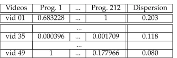
Table 3 shows a representative excerpt of Pre-cision measures that were observed considering the OpenCV case. Similar tables for remaining examples are available in Appendix A. In this table, rows represent test suites and columns are

Videos Prog. 1 ... Prog. 212 Dispersion vid 01 0.683228 ... 1 0.203

...

vid 35 0.000396 ... 0.001709 0.118 ...

vid 49 1 ... 0.177966 0.080

Table 3: Sample of observations for Precision on the OpenCV case

different morphs. As stated before, we used 49 test suites that were executed on 212 morphs. Each cell of the table reports the performance measure of the execution of the program on the video. Based on all retrieved performances for each video, we computed a dispersion score for each individual video which is presented in the last column.

3.3.1 Can different dispersion scores be ob-served?

In the following, we want to validate the fact that we can observe variations in performances inducing different dispersion scores.

OpenCV case. Computed dispersion scores

range from ₂₁₂17 ' 0.08 up to 44

212 ' 0.207. Over

all 49 test suites, the mean value of dispersion scores is ' 0.145 and the standard deviation ' 0.034. While these numbers are rather low (i.e., less than a quarter of the bins are activated), it seems that behaviors of all 212 morphs are not equivalent as shown in Table 3. Meaning that not all morphs give the same performance when executed on the 49 videos8_{. For instance, Prog. 1}

from Table3performs very well on the last video while Prog. 2 is unable to detect anything.

COCO case. In this case, dispersion scores

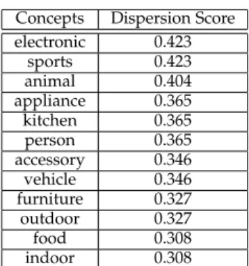
are larger as shown in Table 5. Scores range from 0.308 to 0.423. Among all 12 concepts, the mean value of dispersion scores is ' 0.359 and the standard deviation ' 0.040. Performances of competitors over each concept are available di-rectly on the online leaderboard. Concepts "Elec-tronic" and "Sports" are tied with the maximum dispersion score of 0.423, concepts "Indoor" and "food" are also tied but they are associated with the lower minimum score of 0.308.

Haxe case. Dispersion scores from Table 6

range from ₂₁1 ' 0.047 to 3

21 ' 0.143. Over

all 84 test suites, the mean value of dispersion scores is ' 0.0567 and the standard deviation ' 0.0202. These scores are low, showing con-sistent measures and insignificant differences in the observations. However, those numbers do not indicate the quality of test cases per se. In fact, most of dispersion scores show that only one or two bins are activated in associated histograms.

8. We obtained similar results for the other quantitative properties we have measured such as recall or perfor-mance.

9

In the case where two bins are activated, we assume that retrieved observations lie close to the separation between the two bins. Variations make observations fall sometimes on one side of the separation and sometimes on the other side. Only one test suite, called the core test suite, is associated with the maximum dispersion score. In this test suite, three bins are activated due to variations. We will investigate further this issue in the next research question.

Taking a step backwards, from the differ-ent examples we analyzed, variations in perfor-mances can be shown and captured by the use of dispersion score. Every test suite can give a dis-persion score that is more or less high depicting how different morphs can perform differently on the same test suite. We point out the fact that absolute values of the dispersion score are mean-ingless. Comparing scores given by the COCO case or by Haxe is non-sense as the two cases have nothing in common (i.e., not the same set of morphs, not the same test suites). What is inter-esting is only the order provided by dispersion scores when ranking test suites according to their dispersion score, as discussed in RQ2 Section3.4. 3.3.2 Is dispersion score stable and sensitive to the set of morphs?

Our hypothesis is that the dispersion score as-sociated with test suites only slightly changes depending on morphs considered in the set that is used. In other words, we want to perform a sensitivity analysis about the dispersion score. This analysis is important as it shows that the dispersion scores are not totally dependant on the choices of the morphs. If dispersion scores vary too much when only one morph is used or removed then the dispersion score is pointless since from one run to another, differing in only one change in the set of morphs, the relative importance given to test suites via dispersion scores would be completely different.

To conduct this experiment, we randomly remove some morphs out of the original pool. That is, we only build dispersion scores taking into account the measures coming from remain-ing morphs. Takremain-ing back the OpenCV case: at each iteration it ∈ 0..#_used_₂morphs, we remove it morphs from the original set of morphs and observe the effect on dispersion scores for each 49 videos. The whole process of selecting up to half the morphs and computing dispersion score is repeated 50 times in order to flatten the impact of random choices in the removal of the morphs. Algorithm2describes how measures have been retrieved.

OpenCV case.Figure3 shows the evolution

of the dispersion score of the videos with the best and worst score depending on the number of morphs that have been removed. On this figure,

Algorithm 2 Procedure to assess stability of the

method

(1) current_iter = 1; (2) max_iter = 50;

(3) #_morph_remove = 0;

(4) #_max_morph_remove =#_morph₂ _used

while #_morph_remove = 0 <=

#_max_morph_remove do

for all videos in the set of videos do

while current_iter <= max_iter do

(5) select randomly current_iter morphs to remove;

(6) compute dispersion score w.r.t. re-maining morphs;

(7) store and average dispersion score; (8) store best dispersion score;

(9) store worst dispersion score; (10) current_iter + +; end while (11) current_iter = 1; end for (12) #_morph_remove + + end while

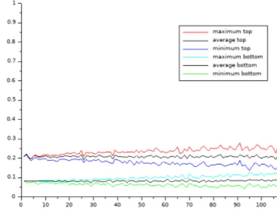
the X-axis represents the number of morphs that have been removed (from 0 to 106) and the Y-axis represents the associated dispersion scores. Six curves are plotted:

• the three top curves represent results for the video providing the best dispersion score;

• the three bottom curves represent results for the video with the worst dispersion scores.

Figure 3: Stability results for the property Preci-sion; X-axis: number of morphs removed; Y-axis: dispersion score

Specifically, considering the best video: (1) The curve in the middle, called average top, reports the average of the dispersion scores, and is obtained through line 7 of Algorithm 2; (2)

the top curve, called maximum top, reports the maximum dispersion score using line 8 of Algo-rithm2; (3) The so-called minimum top reports the minimum dispersion score as defined by line 9 of Algorithm2. We depict the same curves for the worst video.

The average curves, namely average top and average bottomare very stable. The four others (maximum top, minimum top, maximum bottom and minimum bottom) tend to be noisy once fifty morphs or more have been removed. However, despite these variations, none of the curves be-tween the top plots and the bottom ones cross each other. Overall, the results show a stability and consistency in their positions9_.

COCO case We apply the same process on

the COCO dataset but because there are only 52 morphs available, we remove up to 26 morphs instead of 106 which corresponds to remove half our observations. Conclusions are similar to the previous case and dispersion score remains stable and consistent in their positions.

Haxe caseWe run again the same sensitivity

analysis over Haxe. For this case, as we only have a small number of morphs, we remove only up to 10 morphs over the 21 available. Retrieved curves are stable since plateaus appear. Similarly to previous cases (e.g., Fig. 3), top curves and bottom curves never interchange.

3.3.3 How does the dispersion score evolve w.r.t. to the number of bins?

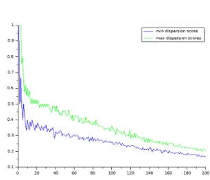
Now that we have assessed the stability of the dispersion score according to the morphs, we can also analyze how it evolves depending on our choice for the number of bins. We focus on the COCO case but conclusions we draw from this case can be generalized to the two others.

Figure 4 shows the evolution of the disper-sion scores associated to test suites that have the minimum (bottom curve) and maximum (upper curve) observed dispersion scores. On the X-axis are the number of bins that we used to compute dispersion scores. We make this number vary from 1 to 200. As a remainder, until now, we have used a rule of thumb which is fixing the number of bins to the number of available morphs. In the COCO case, that was 52 because we had 52 morphs. We also remind that the dispersion score is a ratio from the number of activated bins to the total number of bins. We see that dispersion scores tend to decrease as the number of bins increase. This is due to the ratio: as the number of observations is not increasing, growing the number of bins tends to reduce the result. What is interesting here is that the curves tends to join as the number of bins keep increasing. Indeed,

9. Again, similar observations can be made for other quantitative properties (e.g., Recall, performance or even a composition of different properties).

Figure 4: The evolution of minimum and maxi-mum dispersion scores according to the number of bins (COCO case)

because of the definition, if the number of bins tend towards infinity, all dispersion scores tend towards 0 which makes our dispersion score meaningless. On the other side of the figure, us-ing a small number of bins makes the dispersion scores higher (but their absolute values are mean-ingless) and the differences between the mini-mum and maximini-mum are exacerbated since the minimum dispersion score drops quickly while the maximum dispersion score may stay high a little longer. However, using a low number of bins makes little sense as we want to capture significant differences in morphs’ performances. Indeed, using a small number of bins will create wide bins which would potentially gather signif-icant different performances into the same bin. In Figure4, it looks like from 20 bins the slope tends to be less abrupt which suggests that picking any number from this point might be a good choice. We would advice to avoid choosing a number of bins that is over 140 as the two curves begin to be very close to each other. We are not able to give a straight, clear, general manner to set the number of bins but, in this specific case, we think that any pick in the range [20; 140] might be a good fit. The use of the number of morphs (52) falls into this range and appears to be a reasonable choice for COCO. The sensitivity analysis reported in Figure 4 for COCO has also been performed for OpenCV and Haxe. Empirical results con-firm that number of morphs is relevant, since it lies within the range of suitable number of bins (supplementary material is available online, see Section3.6).

3.4 RQ2: Is the dispersion score a right

mea-sure?

We showed that our dispersion score was able to "rate" test suites with different scores. In the

11

Figure 5: The number of bins activated with the original test suite (composed of 84 test cases). The X-axis represents the index of the bins.

Figure 6: The number of bins activated with the smaller test suite composed of 5 test cases that maximizes the dispersion score. The X-axis represents the index of the bins. Bars in red are bins that are activated with the original test suite showed in Figure5 but that we fail to activate with our smaller test suite.

following, we would like to evaluate whether those scores have the wanted intuitive meaning: is a test suite with a higher score really better than one with a lesser score?

For addressing this qualitative question, we first used an exhaustive search to create an op-timal test suite combining exactly 5 test suites for each of our 3 cases studies. Optimality is defined as maximizing the dispersion score of the new test suite. We then relied on domain specific ground truth to assess whether these "optimal" test suites were indeed any good.

Since the newly built test sets of 5 test suites maximize the dispersion score, we can com-pare our histogram-based representation from the original test set to this one and observe how far they are one to the other. For instance, taking the Haxe case, the histogram of the original test set using 84 test suites is presented in Figure5. Blue light bars represent activated bins. Figure6

shows the histogram of the second test set. Red bars represent differences with Figure 5in acti-vated bins.

Only 4 bins are different between the two histograms, namely bins 3, 6, 18 and 21. Meaning that, at most, 4 test suites are needed, in the reduced test set, to retrieve the same histogram as the original one. In the end, with those

hypothet-ical 9 test suites, we ensure to retrieve the same diversity in the observed quantitative properties but drastically diminishing testing efforts. 3.4.1 (OpenCV case) Can we create a "good" test suite that is able to differentiate morphs that perform well from others?

The selected "optimal" test suite combining 5 test suites was associated with a score of ' 0.6 acti-vating 127 bins over 212 in total. In this regard, this "optimal" test suite is at least 3 times better than any individual test suite. But is it really any good?

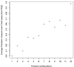
To answer this question, we have asked a CV expert to cherry-pick twelve new morphs in such a way that six of them are expected to perform well on average and six others would be likely to perform poorly/moderately well. Note that we did not ask the expert to choose very bad config-urations that would not recognize anything: since any test suite would be able to tell that they are bad; that would tell us nothing about the relative merit of our test selection process.

Then we ran these 12 morphs on the test suite of 5 videos. For each of these morphs, we plot in Figure7the obtained Precision averaged over the 5 executions. The supposedly 6 moderately poor morphs correspond to index 1 to 6 on the X-axis while indexes 7 to 12 correspond to the 6 others supposed to perform well.

Figure 7: Average Precision measures over the 5 videos from RQ2. On X-axis are the CV morphs: first, the 6 first morphs that are supposed to perform moderately badly; the 6 last morphs are supposed to be good. Y-axis reports the averaged Precision measure over the test suite.

From Figure 7, two classes of programs can be identified: programs which have an average score below 0.4 and programs which reach an average score above 0.5. This separation corrob-orates the expert’s classification since programs

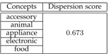
Concepts Dispersion score accessory 0.673 animal appliance electronic food

Table 4: The 5 concepts that maximize the disper-sion score

which reach an average Precision above 0.5 (re-spectively below 0.4) are exactly the ones ex-pected to perform well (respectively moderately poorly). Even if our selected test suite is probably not the best possible one (it is just the best set of exactly 5 test suites), it is already quite able to tell good from poor configurations apart. But is this test suite really better at that than any random test suite of size 5? To answer this question, we created a test suite composed of 5 videos ran-domly picked among our 49 videos. We ran the 12 selected programs on this randomly picked test suite. For each program, similarly as pre-sented in Figure 7, we computed the Precision measure averaged over the test suite. Then, we confront the classification of morphs (depending on whether the average of their performance is above 0.5 or below 0.4) with the intuition of the expert and count how many times they disagree. To mitigate the potential bias induced by random picking, we run this process 10 times. The result is that a minimum of 2 programs out of 12 have been misclassified, with a worst case of 5 misclassified programs.

In average, over the 10 runs, almost 4 pro-grams over 12 are misclassified. The associated standard deviation is 1, suggesting that overall, between 3 and 5 programs are likely to be mis-classified. As a conclusion, we got some evidence that our optimal test suite of 5 videos performs significantly better that a random one of the same size to tell good from poor configurations apart. 3.4.2 (COCO case) Can a smaller test suite built such that it maximizes its dispersion score provide a similar ranking of morphs as the original test suite?

Again, we created a reduced test suite containing 5 concepts following the same process as before. The 5 concepts are presented in Table4and yield a score of 0.673. It is worth noting that it is very close to the dispersion score of the entire COCO benchmark. Note that, once again, the choice of these 5 concepts are not the same as picking the 5 top rows of Table5in Appendix. We have also stated in Section3.3.1that "Sports" and "Electronic" yielded the highest dispersion scores. "Electronic" has been chosen in our minimized test suite but using "Sports" would have been the same as long as it would have activated the same bins.

With this new smaller benchmark, we rank again the competitors. We check that the two rankings are similar in order to assess that not all categories are needed when performing contin-uous evaluations of morphs’ performances. The similarity between the two rankings is estab-lished using the Spearman correlation coefficient. This coefficient indicates whether two ranked lists are strongly correlated when the value is close to 1 or -1, showing whether the evolution follows the same tendency or opposite directions. On the other hand, if the coefficient is close to 0, then no correlation can be deduced.

Table 7 in Appendix provides a compari-son of performances of a sample of competi-tors’ techniques w.r.t. the two benchmarks. The first column presents competitors’ names. We selected 13 techniques out of the 52 competitors that are shown on the leaderboard. That is, we show approximately one out of five techniques. The second column shows the performances pro-vided by the leaderboard. We assume such per-formances to be an average over all 12 concepts.

The third column shows the averaged perfor-mances over the set of 5 concepts (see Table 4) that we retrieved from our method. Finally, the last column shows the absolute difference be-tween the two performances. The differences are rather low which shows how close we are from the original measures but considering fewer data. We also computed some statistics over all 52 techniques which compare the differences be-tween the two set of performances. The aver-age difference in performances over all 52 tech-niques is ≈ 0.013 with a standard deviation of ≈ 0.004. This shows that, most of the time, differ-ences in retrieved performances are in the range [0.01; 0.02] approximately. We also searched for the maximum and minimum differences, they are respectively ≈ 0.025 and 0.008.

Regarding ranks directly: Table 8, in Ap-pendix, shows two rankings on the second and third columns. First, the one retrieved from the COCO leaderboard. Second, the one we com-puted considering our reduced benchmark.The two rankings are similar with only a few ranks that are permuted with the one above or below. The result Spearman correlation coefficient of 0.998 shows a strong correlation between the two rankings.

This strong correlation shows that a small subset selected through to the notion of the dispersion score is nearly as powerfull as the full test suite to rank competitors. The concrete consequence of that is out of all concepts in COCO, only a smaller number is needed to assess the global behavior of competitors. In the end, their continuous evaluations could be reduced to assess performances on a smaller number of concepts such that competitors can get an idea of

13

their rank in the competition more quickly, with fewer resources which in turn could help them improve their solutions more quickly and more frequently.

3.4.3 (Haxe case) Can we discover bugs thanks to the dispersion score? Can we build a smaller test suite that is able to select interesting test cases?

For this case, we want to check that a higher dispersion score might be correlated with the detection of performance bugs. In particular, we focus on the test suite with a maximal dispersion score that had activated 3 bins.

Because most dispersion scores activated one or two bins, we assumed that performances ob-served lied close to a boundary between those two bins and little variations caused observa-tions to lie sometimes in one bin and sometimes in another. However, when three bins are acti-vated, it is unlikely that little variations could cause this behavior. There must be something else: we analyzed observations of the test suite associated with the highest retrieved dispersion score. Retrieved performance were rather consis-tent except for code generator variants targeting the PHP language. Performances regarding those morphs drastically increased. In fact, execution times were at least 40 times longer than for morphs targeting other languages. Checking re-sults with authors from previous work [16], [17], they also have noticed this anomaly and reported it to Haxe community in a bug report. Developers responded that they knew about it, it was fixed already but the patch was not live when [16], [17] conducted their study.

3.5 Concluding remarks over the method

We can answer the main research questions.

Performance diversity (RQ1).Is our

disper-sion score able to capture different performance values and thus assign different scores to differ-ent test suites? We showed we are able to build a dispersion score that assigns a higher value to test suites able to capture significant differences in performance values. The ranges of dispersion scores are as follows: the OpenCV case showed dispersion scores ranging from 0.08 to 0.207. The minimal score of 0.08 is assigned to a test suite on which most of OpenCV morphs performed sim-ilarly. On the other hand, with a score of 0.207, about a fifth of morphs performed significantly different on this test suite. Regarding COCO and Haxe, dispersion scores ranged respectively from 0.308 to 0.423 and from 0.047 to 0.143. For every case studies, dispersion scores were able to dif-ferentiate test cases by assigning them different dispersion score whether they are able to capture more or less different performance values.

Stability (RQ1). Are dispersion scores very

sensitive to the use of particular morphs? Our sensitivity analysis showed that dispersion scores were rather stable regardless of used morphs. Hence our method is able to deal with morphs having similar performances; we can certainly avoid the costly use of some equivalent morphs. It also suggests that our method is robust even when the selection of morphs is realized in an agnostic way being the use of random selection. However, we cannot claim that domain knowl-edge will not be beneficial to our method (e.g., for selecting optimal configurations and morphs, see discussions in Section4).

Applicability (RQ2). Can dispersion scores

be correlated with an external evaluation, specific to each case, of what would be "good" test suites? We showed that, dispersion scores can be used to rank test suites in order of importance w.r.t. the different performance values they are able to capture. They can also be used to build smaller test suites than the original that will maximize this score. With smaller test suites, we were able to:

• execute a set of OpenCV morphs se-lected by a Computer Vision expert and match the intuition of the experts regard-ing morphs’ behaviors (i.e., the 6 morphs supposed to perform better according to the expert were indeed the ones perform-ing the best on our smaller test suite com-posed of 5 test cases);

• retrieve a similar ranking of COCO

com-petitors as the original one, that is avail-able online, with a strong Spearman corre-lation coefficient (i.e., 0.998) between the two rankings. Our test suite took into account 5 of the 12 concepts originally present in the COCO dataset;

• exhibit a bug in generated PHP code with

only 5 test suites out of the 84 composing the original test suite. Of course, this bug was already found by the original test suite. From previous studies [16], [17], this bug was the only one to be found via a comparison of performances. By applying Multimorphic Testing, we were able to re-duce the size of the test suite while keep-ing its ability to show this performance bug.

3.6 Reproducibility of experiments

Data, code and results are available in a public repository on Github at the following link:https:

//github.com/templep/TSE_MM_test.git.

For practitioners interested in reproducing the analysis of our data, we provide all configu-rations, test suites and observations through CSV files. Statistical results presented this article are

available through text files or plots. The code for producing such results is written in Scilab, an open-source software close to Matlab and is also included. For OpenCV and Haxe practitioners interested in reproducing the computations of performance data, we provide specific instruc-tions as well as the code to instrument the whole process.

4

D

T

V

4.1 Internal threats

To compute our dispersion score, we used a 2D representation inspired from histograms. Despite not being interested in the actual frequency value of each bin, we need to know which one are activated to compute our dispersion score. On the X-axis, the representation defines bins and their number is crucial in our method. Defining the right number of bins remains an open question since it depends on the application: trying to analyze a color distribution of an image, com-paring two different data distribution requires a very fine-grained analysis and thus a larger number of bins; while, in our case, requirements are different. Using a small number of bins would provide a coarse analysis of the variability in the results while more bins might isolate every execution into its own single bin and thus would show differences that are not significant. We fixed the number of bins to the number of used morphs as a reasonable trade-off, but this is only true if the number of morphs is large enough.

In RQ2, we validate the usefulness of our dispersion score by building test suites composed of 5 test cases that maximized the dispersion scores. 5 is an arbitrary value chosen to limit the amount of time taken by the exhaustive search. For example, in the OpenCV case, 5 test suites among 49 result in 49!/(5! ∗ (49 − 5)!) combinations which is about 1.9M combinations. Increasing the number of test suites that we take into account drastically increases the number of combinations, for instance, taking 7 instead of 5 results in about 85.9M combinations. We are aware that, depending on the application do-main, the number of test cases to consider may vary and 5 is certainly not the optimal number to use in every occasion. 5 has no value per se in our experiments except that it allows us to make computation time affordable for our validation. Even with such a small number, we already get interesting enough results to be able to conclude on the potential of our technique.

In the sensitivity analysis, we analysed the effect of removing half of the morphs. This choice is arbitrary but seems reasonable to demonstrate the stability of the dispersion score and compare it with the use of all morphs. It is an open

question how many morphs should be chosen to obtain a relevant score.

In the end, our dispersion score, the represen-tation and exhaustive search are only one way to instantiate the Multimorphic testing approach. Even if it seems to work surprisingly well, at least for the different application we have considered, other options might perform better and need to be explored.

4.2 External threats

Applicability. Can Multimorphic testing and

our proposed dispersion score be used in ferent domains? Our experiments took three dif-ferent application domains that are tracking of objects in videos, object recognition in images and program generation. The method was able to detect test suites emphasizing interesting behav-iors of morphs. While two application domains are rather close, associated tasks were different. Results presented in Section3 mitigate this first threat as it shows that, at least in presented situations, Multimorphic testing can be applied.

Performance dimensions and metrics.About

generalization, we presented results regarding only one performance measure at a time, namely Precision or execution time. Further experiments have been running taking into account other measures such as Recall or memory consumption or even a combination of Precision and Recall or Precision and execution time, similar conclusions were drawn from those extra experiments but we do not show them in this document as it would not provide more insights about the method. They are available on the companion GitHub repository though.

On test suites (OpenCV). Regarding the

OpenCV case specifically, test sets were com-posed of synthetic videos only. The merit of synthetic videos is that (1) the associated ground truths are of high quality (by construction since they are synthesized); (2) we can better control the properties of the videos and thus increase the diversity of situations. Synthetic videos are getting more and more used in the industry or in research as a substitute or complement of real assets [9], [18], [19], [20]. However, natural videos may not provide as diverse behaviors and per-formance measurements as we observed. Note that other experiments like the COCO case used "natural" images and still gave fairly good results which mitigates this threat.

On test suites (Coco).Focusing on the COCO

dataset, we did not have access to raw images; we only considered concepts and classes of objects. It seems realistic to assume that object classes are not equally represented over all the images of the dataset. For instance, there might be fewer objects labeled "hair dryer" than objects labeled "cat". A hypothesis is that classes that are more

15

represented might have more chances to pro-vide "extra diversity" and thus to show differ-ences among competing approaches. Results we present in Section3might be biased as they could simply reveal that the reduced set of 5 concepts is composed of the 5 most represented ones. However, it is only a hypothesis that does not necessarily hold in general, i.e., there is not neces-sarily a correlation between the size of the dataset and performance diversity. For COCO, we can hardly validate this hypothesis since concepts are coarse abstractions averaging performances of large subsets of images. In any case, we have shown that our method is able to retain the key elements of the dataset that exhibit diversity within the performances of competing systems.

Data preprocessing. In the Haxe case, our

evaluation is based on results from prior mea-sures performed on the same Haxe code gener-ator. Measures that we retrieved were prepro-cessed (as explained in3.2.3) which might exac-erbate or alleviate differences in observed perfor-mances. However, the fact that we were able to retrieve a test suite that highlighted the presence of a bug in PHP generated code is encouraging. Furthermore, the fact that measures were consis-tent, with only one or two bins activated, shows that the dispersion score is somehow invariant to this preprocessing. Further investigations should be conducted in order to understand which kind of preprocessings do not affect drastically the dispersion score.

Morphs’ selection The ability of

Multimor-phic Testing to observe different performance behavior is dependent of the nature of morphs. Using only very similar morphs (with only a small delta in the value of one parameter) might not be enough to observe differences while the morphs will be different in their configurations. Used morphs should be somehow representative of the whole population of morphs of a sys-tem. This is an assumption that we used for all our experiments: we have generated morphs of OpenCV for a specific task with the goal of ex-ploring the configuration space as much as pos-sible; we considered competitors to the COCO competitions to be representative of the state-of-the-art techniques in terms of object recognition; and similarly for the Haxe case, we considered that target languages and optimization options to be representative of what users might look for. The underlying problem is how to sample those morphs efficiently? This remains an open problem in the Software Product Lines commu-nity that is addressed by several works, mainly for finding functional bugs [21], [22], [23], [24]. Overall, a threat to the adoption of multimor-phic testing is that the process can be highly computational demanding for some domains; an optimal selection of morphs and reduction of

per-formance test suites are open research directions worth exploring.

5

R

W

This paper proposes to proactively create morphs, also called variants in the Software Product Lines community, for the purpose of assessing the quality of a test suite. We have evaluated our approach in different application domains. Our contribution is thus at the cross-road of software testing (including mutation and metamorphic testing10), variability management, compilers, and computer vision.

5.1 Software testing

Software testing techniques have been developed to assess, optimize, or generate a test suite. The general idea is that a test suite could be evaluated according to a certain criterion, e.g., a code cover-age criterion describing a set of structural aspects of a program, like statements, lines or branches. Search-based techniques are particularly used to explore this search space to find the input data that maximize the given objective [25] (e.g., cover as many branches as possible [26]). Black-box or white-box software testing techniques have been proposed [27]. The idea is to generate random inputs while observing resulting outputs, typ-ically for detecting failures. Whitebox fuzzing, such as SAGE, consists of executing the program and gathering constraints on inputs [28]. SAGE exploits constraints to guide the test generation.

While load testing techniques have been de-veloped to evaluate the performance of sys-tems [29], [30], no such testing criteria exist for quantitative properties. We developed a dedi-cated process and criterion that can be defined in terms of performance dispersion of morphs. Based on such a criterion, we can envision to optimize test suites using, for instance, search-based techniques.

Mutation analysis is a well-known technique for either evaluating test suite quality or support-ing test generation [31], [32], [33], [25]. Artificial defects, known as mutations, are injected into the program yielding mutants; one can then measure test effectiveness based on the number of “killed” mutants that have failed tests. Multimorphic test-ing pursues similar goal as mutation testtest-ing, i.e., assessment of the strength of a test suite, with our morphs playing a similar role as mutants do in mutation analysis. There are two impor-tant differences. First, we do not rely on typical

10. Actually some people say that what we are doing here is mutation testing, while others say equally strongly that it is metamorphic testing, and still others say it is neither. We thus forged a new term, Multimorphic testing, but if there is a consensus among the reviewers that this is either mutation testing or metamorphic testing, we would be happy to acknowledge and change our title.