DOI:10.22055/JACM.2018.24959.1221 jacm.scu.ac.ir
Heat Transfer in Hydro-Magnetic Nano-Fluid Flow between
Non-Parallel Plates Using DTM
Mohamed KEZZAR
1,2, Mohamed Rafik SARI
1, Rabah BOURENANE
1, Mohammad Mehdi
RASHIDI
3, Ammar HAIAHEM
11 Laboratory of Industrial Mechanics, Badji Mokhtar University of Annaba, B.O. 12, 23000 Sidi Amar Annaba, Algeria 2 Mechanical Engineering Department, University of Skikda, El Hadaiek Road, B. O. 26, 21000 Skikda, Algeria 3 Department of Civil Engineering, University of Birmingham, Edgbaston Birmingham B15 2TT, United Kingdom
Received February 10 2018; Revised April 16 2018; Accepted for publication April 27 2018. Corresponding author: Mohamed KEZZAR, [email protected]
Copyright © 2018 Shahid Chamran University of Ahvaz. All rights reserved.
Abstract. This study presents a computational investigation on heat and flow behaviors between non parallel plates
with the influence of a transverse magnetic field when the medium is filled with solid nanoparticles. The nonlinear
governing equations are treated analytically via Differential Transform Method (DTM). Thereafter, obtained DTM
results are validate with the help of numerical fourth order Runge-Kutta (RK4) solution. The main aim of this research
work is to analyze the influence of varying physical parameters, in particular Reynolds number, nanofluid volume
fraction, and Hartmann number. It was found that the presence of solid nanoparticles in a water base liquid has a
notable effect on the heat transfer improvement within convergent-divergent channels. The comparison of DTM
results with numerical RK4 solution also shows the validity of the analytical DTM technique. In fact, results
demonstrate that the DTM data match perfectly with numerical ones and those available in literature.
Keywords: Nanofluid Flow; Hydromagnetics; Convergent-Divergent Channel; DTM; Skin friction; Nusselt.
1. Introduction
The celebrated Jeffery-Hamel flow is highly recognized as one of the rare exact solutions of the Navier-Stokes equation that describes the two-dimensional flow within convergent-divergent channels. The nonlinear mathematical equation of this flow was firstly proposed by Jeffery [1] in 1915 and independently by Hamel [2] in 1916. Thereafter, an increasing interest was dedicated to the Jeffery-Hamel flow due to its numerous engineering applications such as fluid mechanics in addition to chemical, biomechanical, and mechanical engineering. The flow within convergent-divergent channels was also the subject of several contributions [3-7] which explains why the literature is so rich with this kind of flow.
Hydromagnetics or Magneto-Hydrodynamics (M.H.D.) is a branch of science which studies the dynamics of electrically conducting fluids. Magneto-hydrodynamic has several industrial applications such as MHD power generation, crystal growth, accelerometers, designing cooling systems with liquid metals, and flow meters. The effect of magnetic field on heat and fluid flow in many geometries has attracted the researchers’ community and investigated by many them [8-11].
Nowadays, it is highly established that the heat transfer improvement in engineering systems is mainly restricted by the lower thermal conductivity of the base liquids like oils, kerosene and water, etc. This lower thermal conductivity is therefore a serious problem which can easily limit the performance and reliability of engineering components such as electronic devices and heat exchangers. To overcome this restriction and limitation, a novel category of fluids, called nano-fluids, created by dispersing small solid particles (less than 100 nm) like Al2O3, Cu and CuO in a conventional base liquid, is proposed as an alternative
technological solution. In fact, nano-fluids can be considered as a superior class of solid-liquid suspensions due to the anomalously higher thermal conductivities of solid nanoparticles. The nano-fluid term was firstly employed by Choi [12] in
Heat Transfer in Hydro-Magnetic Nano-Fluid Flow Between Non Parallel Plates Using DTM
1995. Since then, nano-fluids have received a considerable interest and investigated numerically and experimentally by many authors. By numerical means, studies are focused on heat and nano-fluid flow analysis in many geometries. Noreen Sher Akbar [13] studied free convective peristaltic motion of hydromagnetic Jeffery nano-fluid in an irregular channel. This investigation used homotopy perturbation method to solve the governing equations. Turkyilmazoglu [14] presented a rescaling approach that significantly simplified the evaluation of flow and physical characteristics in a recent single phase of nano-fluids research. The presented approach mainly allowed to view certain nano-fluid flows in terms of standard fluid flows. Turkyilmazoglu [15] also studied the traditional laminar plane wall jet when the medium was filled with different types of solid nanoparticles. This numerical investigation mainly shows the effects of nano-fluids on the heat and flow behaviors of the wall jet. Mohebbi and Rashidi [16] investigated the natural convection heat transfer through L-shaped enclosure in the presence of an internal heating in the steady Al2O3-Water nano-fluid flow. This investigation used the Latrtice Boltzmann Method (LBM) to solve the governing
mathematical equations. Using Boungiorno’s two phase model, the conjugate free convection flow and thermal behavior in a heat exchanger were performed by Garoosi and Rashidi [17]. Heat and fluid flow within convergent-divergent channels in the presence of copper solid nanoparticles in a water base were studied by Sari et al. [18]. In another work, Kezzar and Sari [19] also carried out an analytical study on heat and nano-fluid flow within stretchable/shrinkable convergent-divergent channels when the medium is filled with Al2O3 solid naoparticles. Rashidi et al. [20] performed a study showing the simultaneous effect
of magnetic field and solid nanoparticles when studying micropolar fluid flow between parallel plates. Ramly et al. [21] also studied the axisymmetric thermal radiative boundary layer flow of nano-fluid over a stretched sheet. They investigated the effects of zero and nonzero fluxes on the distributions of temperature and volumetric fraction of nanoparticles. Experimentally, the conducted studies [22, 23] were focused on the measurements of nano-fluids thermal conductivity. These experimental studies mainly described that the nano-fluids depict significantly higher thermal conductivities when compared to that of base liquids. In recent decades, a wide variety of robust approximate analytical techniques were developed such as the Homotopy Analysis Method (HAM), the Adomian Decomposition Method (ADM), the Variational Iteration Method (VIM), and the Differential Transform Method (DTM). These methods were successfully employed for solving mathematical or physical linear and non-linear differential equations. Thereafter, several modifications were adopted to these techniques in order to enhance their efficiency. For example, Turkyilmazoglu [24] developed a new optimal variational method which is successfully applied for heat and fluid flow problems. Moreover, Turkyilmazoglu [25] give an elegant modification of the traditional Adomian decomposition method by introducing a convergence control parameter into the method.
As mentioned above, DTM method is one of several robust approximate analytical techniques which was first introduced by Zhou [26] in 1986. Generally, DTM technique gives the solution as a polynomial series and can be directly implemented without requiring linearization, discretization, or any perturbation. According to the literature, we can find a wide number of studies using Differential Transform Method. For example, Rashidi and Erfani [27] employed DTM method to investigate nonlinear heat and Burgers' equations. The reliability of this investigation is tested by comparing the results obtained with those of available HAM solution. Rashidi et al. [28] carried out an investigation on heat transfer in the unsteady M.H.D flow over a stretching surface considering viscous dissipation. They constructed analytical approximate solutions using DTM method and the Padé approximants. Sheikholeslami and Ganji [29] also analyzed heat and fluid flow between parallel plates via DTM method and with the influence of some important physical parameters of the considered problem.
The main goal of this contribution is to investigate the effect of varying physical parameters, in particular nano-fluid volume fraction (), Reynolds number (Re), and Hartmann number (Ha) on heat transfer in the steady nano-fluid flow within convergent-divergent channels. The nonlinear governing equations of the studied problems are treated analytically via Differential Transform Method (DTM) and numerically using a fourth order Runge Kutta method featuring the shooting technique. Furthermore, the obtained analytical DTM results are compared with numerical RK4 solution, exact solution, and those reported in literature in order to test the validity and reliability of DTM solution.
2. Basic Equations
This contribution is devoted to the flow and heat transfer analysis in the steady two-dimensional flow of an incompressible nano-fluid within convergent-divergent channels. For the considered nano-nano-fluid flow, the symmetric nature is adopted. Moreover, the flow is considered to be uniform along z-direction and the velocity is assumed purely radial and mainly depended on r and coordinates. In this situation, the fluid velocity is given as follows (𝑉 = 𝑉(𝑟, 𝜃), 𝑉 = 0, 𝑉 = 0). Moreover, as drawn in Fig. 1, it is obvious that the magnetic field acts transversely to the flow direction.
In cylindrical coordinates (r, , z), the momentum and energy equations of the considered hydromagnetic nano-fluid flow within convergent-divergent channels are given as [4]:
𝜌 𝑟 . 𝜕 𝜕𝑟(𝑟. 𝑉 ) = 0 (1) 𝑉 .𝜕𝑉 𝜕𝑟 = − 1 𝜌 . 𝜕𝑃 𝜕𝑟+ 𝜈 . 𝜕 𝑉 𝜕𝑟 + 1 𝑟. 𝜕𝑉 𝜕𝑟 + 1 𝑟 . 𝜕 𝑉 𝜕𝜃 − 𝑉 𝑟 − 𝜎𝐵 𝜌 𝑟 𝑉 (2) − 1 𝜌 . 𝑟. 𝜕𝑃 𝜕𝜃+ 2. 𝜈 𝑟 . 𝜕𝑉 𝜕𝜃 = 0 (3) (𝜌. 𝑐 ) 𝑉𝜕𝑇 𝜕𝑟 = 𝐾 1 𝑟 𝜕 𝜕𝑟 𝑟 𝜕𝑇 𝜕𝑟 + 1 𝑟 𝜕 𝑇 𝜕𝜃 + 𝜇 2. 𝜕𝑉 𝜕𝑟 + 𝑉 𝑟 + 1 𝑟 𝜕𝑉 𝜕𝑟 + 𝜎. 𝐵 . 𝑉 𝑟 (4)
where 𝑉 , P, T, 𝜎, and 𝐵 represent the radial velocity, pressure, temperature, fluid conductivity, and electromagnetic induction, respectively. In addition, 𝜌 ,𝜇 ,𝜈 ,𝑐 , and 𝐾 characterize the density, dynamic viscosity, kinematic viscosity, heat capacity, and effective thermal conductivity of nano-fluid, respectively. With the relevant boundary conditions as:
𝑉 = 𝑉 , = 0, = 0 at 𝜃 = 0 (5)
𝑉 = 0, 𝑇 = 𝑇 at 𝜃 = 𝛼 (6)
𝑇 characterizes the wall temperature. The quantities 𝜌 ,𝜇 , and (ρ. Cp) are given as in Dogonchi et al. [30]: 𝜌 = (1 − 𝜓)𝜌 + 𝜓. 𝜌 𝜇 = ( ) . (𝜌. 𝑐 ) = (1 − 𝜓). (𝜌. 𝑐 ) + 𝜓. (𝜌. 𝑐 ) = ( ) ( ) (7)
where is the nano-fluid volume fraction. The subscript '' f '' characterizes the base fluid and '' s '' denotes the solid nanoparticles. For a purely radial motion, Eq. (1) yields:
𝑓(𝜃) = 𝑟. 𝑉 (8)
Consider the following variables [4]:
𝑓(𝜂) = ( ), 𝑔(𝜂) = 𝑟 . (𝜂 = 𝜃/𝛼) (9) where 𝑓 is the centerline rate of the movement (𝑓 = 𝑟. 𝑉 ). Substituting variables of Eq. (7) into Eqs. (2) and (3) and eliminating P term between the obtained equations leads to:
𝑓 + 2𝑅 . 𝛼. (1 − 𝜓) . . ((1 − 𝜓) + 𝜓.𝜌
𝜌 ) . 𝑓𝑓 + (4−(1 − 𝜓)
. 𝐻𝑎) 𝛼 𝑓 = 0 (10)
Besides, introducing Eq. (7) into Eq. (4) yields 𝑔 + 4𝛼 𝑔 +𝐴 𝐵2𝛼 𝑃 𝑓𝑔 + 𝑃 . 𝐸 𝑅 . 𝐵. (1 − 𝜓) . (4𝛼 𝑓 + 𝑓 ) + 𝑃 . 𝐸 𝐻𝑎 𝐵 𝑓 = 0 (11) where 𝐴 = (1 − 𝜓) + 𝜓.𝜌 . 𝑐 𝜌 . 𝑐 (12) 𝐵 = 𝑘 + 2𝑘 − 2𝜓(𝑘 − 𝑘 ) 𝑘 + 2𝑘 + 𝜓(𝑘 − 𝑘 ) (13)
In terms of normalized functions 𝑓(𝜂) and 𝑔(𝜂), the boundary conditions become:
𝑓(0) = 1 , 𝑓 (0) = 0 , 𝑔 (0) = 0 at 𝜂 = 0 (13)
Heat Transfer in Hydro-Magnetic Nano-Fluid Flow Between Non Parallel Plates Using DTM
It should be mentioned that the studied problem represented by Eqs. (10), (11), (13), and (14) can be reduced to the case of a traditional nano-fluid flow within convergent-divergent channels when Ha=0. The dimensionless quantities presented in the above-mentioned Eqs. (10) and (11) are:
Reynolds number 𝑅 = . Prandtl number 𝑃 = . . Eckert number 𝐸 = . . Hartmann number 𝐻 = (15a-d)
Physical parameters that characterize the studied problem are the skin friction coefficient and the Nusselt number. The skin friction coefficient 𝐶 is given by:
𝐶 = 𝜏
𝜌 . 𝑉 (16)
The wall shear stress 𝜏 is given as
𝜏 = 𝜇 . (1 𝑟.
𝜕𝑉
𝜕𝜃) (17)
The Nusselt number Nu is defined as
𝑁𝑢 =𝑟. 𝑞 |
𝐾 . 𝑇 (18)
where 𝑞 is the heat flux which is expressed as:
𝑞 = −𝐾 . ( + . ) (19)
Using Eq. (7), it yields:
𝐶 = 1 𝑅.. (1 − 𝜓) . . 𝑓 (1) (20) 𝑟 . 𝑁𝑢 =𝐾 𝐾 . [2 − 𝑔 (1) 𝛼 ] (21)
3. Basic Idea of DTM method
For one dimensional problem, differential transformation of the function g() is given as follows: 𝐺(𝑘) = 1
𝑘![ 𝑑 𝑔(𝜂)
𝑑𝜂 ] (22)
where 𝐺(𝑘) is the transformed function and g() is the original function. The transformed function represents the spectrum of the original function g(). The inverse transformation is:
𝑔(𝜂) = 𝐺(𝑘). (𝜂 − 𝜂 ) (23)
The combination of Eqs. (22) and (23) yields:
𝑔(𝜂) = [𝑑 𝑔(𝜂) 𝑑𝜂 ] .
(𝜂 − 𝜂 )
𝑘! (24)
It can be deduced from Eq. (24) that the concept of DTM technique is derived from Taylor's series expansion, however, the derivatives are not evaluated symbolically by the DTM method. In fact, the derivatives are evaluated via an iterative scheme which is well described by the transformed equations of the original functions. For real applications, the function g() may be expressed as a finite series as follows:
where N is the series size. Equation (25) implies that ∑ 𝐺(𝑘). (𝜂 − 𝜂 ) is very small and consequently neglected. Finally, the mathematical operations given in Table 1 are deuced from the mathematical formulations (22) and (23).
Table1. Differential Transformation operations Original function Transformed function
f g h F k
G k
H k
n
n d g f d F k
k n !
G k
n
k ! ( ) ( ) ( ) f g h F k[ ]
km0F m H k[ ] [ m] ( ) sin( ) f
[ ] sin( ) ! 2 k k F k k ( ) cos( ) f
[ ] cos( ) ! 2 k k F k k f ( ) e [ ] ! k F k k
( ) 1 m F [ ] ( 1)...( 1) ! m m m k F k k ( ) m f [ ] ( ) 1 , 0 , k m F k k m k m 4. Implementation of DTM
The DTM method is applied to Eqs. (10) and (11) that describe the studied nonlinear problems. By taking the differential transforms of Eqs. (10) and (11), the following relations is obtained:
(𝑘 + 1)(𝑘 + 2)(𝑘 + 3)𝑭(𝑘 + 3) + 2𝑅 . 𝛼. (1 − 𝜓) . . (1 − 𝜓) + 𝜓.𝜌 𝜌 . (𝑘 + 1)𝑭(𝑘 + 1 − 𝑙)𝑭(𝑙) + (4−(1 − 𝜓) . 𝐻𝑎) 𝛼 (𝑘 + 1)𝑭(𝑘 + 1) = 0 (26) (𝑘 + 1)(𝑘 + 2)𝑮(𝑘 + 2) + 4𝛼 𝑮(𝑘) +𝐶 𝐶 2𝛼 𝑃 . 𝑭(𝑘 − 𝑙)𝑮(𝑙) + 𝑃 . 𝐸 𝑅 . 𝐶 . (1 − 𝜓) . 4𝛼 . 𝑭(𝑘 − 𝑙)𝑭(𝑙) + . (𝑘 + 1)(𝑘 + 1)𝑭(𝑘 + 1 − 𝑙)𝑭(𝑙 + 1) +𝑃 . 𝐸 𝐻𝑎 𝐶 . . 𝑭(𝑘 − 𝑙)𝑭(𝑙) = 0 (27)
where F(k) and G(k) are the differential transforms of f(η) and g(η). The transformed boundary conditions are:
𝐹(0) = 1, 𝐹(1) = 0, 𝐹(2) = 𝑎 (28)
𝐺(0) = 𝑏, 𝐺(1) = 0 (29)
where a and b are the constants which may be determined from the boundary conditions (28) and (29). Using DTM, the studied nonlinear mathematical equations can be solved as follows:
For nano-fluid flow (i.e. fluid velocity)
𝐹(0) = 1 𝐹(1) = 0 𝐹(2) = 𝑎 𝐹(3) = 0 𝐹(4) = −1 3𝑎𝛼 − 1 6𝑐Re𝛼(1 − 𝜓) . + 1 12𝑎Ha𝛼 (1 − 𝜓) . +1 6𝑎Re𝛼(1 − 𝜓) . 𝜓 − 1 6ρ 𝑎Reρ 𝛼(1 − 𝜓) . 𝜓 𝐹(5) = 0 (30)
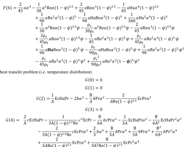
Heat Transfer in Hydro-Magnetic Nano-Fluid Flow Between Non Parallel Plates Using DTM 𝐹(6) = 2 45𝑎𝛼 − 1 30𝑎 Re𝛼(1 − 𝜓) . + 2 45𝑎Re𝛼 (1 − 𝜓) . − 1 45𝑎Ha𝛼 (1 − 𝜓) . + 1 90𝑎Re 𝛼 (1 − 𝜓) .− 1 90𝑎HaRe𝛼 (1 − 𝜓) .+ 1 360𝑎Ha 𝛼 (1 − 𝜓) . + 1 30𝑎 Re𝛼(1 − 𝜓) . 𝜓 − ρ 30ρ 𝑎 Re𝛼(1 − 𝜓) . 𝜓 − 2 45𝑎Re𝛼 (1 − 𝜓) . 𝜓 + 2ρ 45ρ 𝑎Re𝛼 (1 − 𝜓) . 𝜓 − 1 45𝑎Re 𝛼 (1 − 𝜓) .𝜓 + ρ 45ρ 𝑎Re 𝛼 (1 − 𝜓) .𝜓 + 1 90𝑎𝐇𝐚Re𝛼 (1 − 𝜓) .𝜓 − ρ 90ρ 𝑎HaRe𝛼 (1 − 𝜓) .𝜓 + 1 90𝑎Re 𝛼 (1 − 𝜓) .𝜓 − ρ 45ρ 𝑎Re 𝛼 (1 − 𝜓) .𝜓 + ρ 90ρ 𝑎Re 𝛼 (1 − 𝝍) .𝜓
For heat transfer problem (i.e. temperature distribution) 𝐺(0) = 𝑏 𝐺(1) = 0 𝐺(2) =1 𝐴EcHaPr − 2𝑏𝛼 − B 𝐴𝑏Pr𝛼 − 2 𝐴Re(1 − 𝜓) . EcPr𝛼 𝐺(3) = 0 𝐺(4) = 2 A𝑐EcHaPr − 1 3A(1 − 𝜓) . Re𝑐 EcPr − B 6A𝑏𝑐Pr𝛼 − 1 3𝐴EcHaPr𝛼 − B 6A EcHaPr 𝛼 − 2 3A(1 − 𝜓) . Re𝑐EcPr𝛼 + 2 3𝑏𝛼 + B 3𝐴𝑏Pr𝛼 + B 3A𝑏Pr𝛼 + B 6A 𝑏Pr 𝛼 + 2 3𝐴Re(1 − 𝜓) . EcPr𝛼 + B 3A Re(1 − 𝜓) . EcPr 𝛼 (31)
Finally, by substituting systems of Eqs. (30) and (31) into the main differential transformation Eq. (25), the solution of the studied problems takes the following forms:
𝑓(𝜂) = 𝐹(0) + 𝐹(1). 𝜂 + 𝐹(2). 𝜂 + ⋯ + 𝐹(𝑁). 𝜂 (32)
𝑔(𝜂) = 𝐺(0) + 𝐺(1). 𝜂 + 𝐺(2). 𝜂 + ⋯ + 𝐺(𝑁). 𝜂 (33)
where N is the series order.
5. Results and Discussion
In this study, the hydro-magnetic nano-fluid flow and heat transfer between non parallel plates is studied analytically and numerically. Analytical solution of the mathematical equations (Eqs. 26 and 27) governing the studied nonlinear problems with transformed boundary conditions is computed by means of Differential Transformation Method (DTM), while numerical solution is gained via the fourth order Runge-Kutta method. In this investigation, a comparative study between analytical and numerical results is also made in order to validate DTM solution.
The present study shows the influences of varying physical parameters like Reynolds number (Re), Hartman number (Ha), and nano-fluid volume fraction () on flow and heat transfer behaviors. The thermo-physical characteristics of all considered nanoparticles (CuO, TiO2, Al2O3 and Cu) are summarized in Table 2.
Table 2. Thermophysical characteristics of considered solid nanoparticles base liquid ρ (Kg/m3) Cp (J/Kg.°K) K (W/m.°K)
Water 997.1 4179 0.613
Alumina, Al2O3 3970 765 40
Copper, Cu 8933 385 400
Titanium dioxide, TiO2 4250 686.2 8.9538
Copper Oxide, CuO 535.6 6500 20
The effects of Reynolds number on the velocity profile and temperature distribution for Copper-Water nano-fluid flow within convergent-divergent channels are depicted in Figs. 2, 3, 4, and 5. As drawn in Fig. 2, for a convergent channel when =-3°, Ha=110, Ec=0.5, and =0.1, the nano-fluid velocity raises as the Reynolds number raise. In fact, at the level of centerline of channel, a flatter profile is observed with high gradients near the walls. In this situation, it is clearly noted that the thickness of momentum boundary layer become smaller with the raise of Reynolds number. In the case of divergent channel, when =+3°, Ha=110, Ec=0.5, and =0.1, as displayed in Fig. 3, it appears that the nano-fluid velocity become smaller as the magnitude of Reynolds number raise. Moreover, Fig. 3 depicts that the volume flux is concentrated at the center of divergent channel with a smaller gradient observed near the walls. Consequently, the thickness of momentum boundary layer raises considerably. In addition, the obtained results also display that the backflow is occurred in the divergent channel, but it is entirely excluded in the
convergent channel. On the other hand, Fig. 4 depicts the variation of thermal profile versus Reynolds number in a convergent channel when =-3°, Ha=110, Ec=0.5, and =0.03. It is noticed that the temperature raises with the raise of Reynolds number and accordingly leads to a decrease in the thickness of thermal boundary layer.
Fig. 2. Velocity distribution vs Reynolds number in converging channel- case of Cu-water nano-fluid flow when α = - 3°, Ec = 0.5,
Ha=110, and ψ = 0.03.
Fig. 3. Velocity distribution vs Reynolds number in diverging channel- case of Cu-water nano-fluid flow when α = + 3°, Ec = 0.5,
Ha=110, and ψ = 0.03.
Fig. 4. Thermal distribution vs Reynolds number in converging channel - case of Cu-water when α =- 3°, Pr=7, Ec = 0.5, Ha=110,
and ψ = 0.03.
Fig. 5. Thermal distribution vs Reynolds number in diverging channel - case of Cu-water nano-fluid flow when α =+3°, Pr=7, Ec
= 0.5, Ha=110, and ψ = 0.03.
For a divergent channel, the influence of Reynolds number on the thermal behavior, when =+3°, Ha=110, Ec=0.5, and =0.03, is drawn in Fig. 5. In fact, it can be clearly observed that the temperature decreases with the raise in Reynolds number. Consequently, the thermal boundary layer thickness raises. The effects of Hartmann number, Ha, on the evolution of velocity and temperature within convergent-divergent channels are given in Figs. 6-9. Indeed, Figs. 6 and 7 depict that the fluid velocity has a direct relationship with the Hartmann number. It can be observed that the velocity raises as the Hartmann number raise. From these Figures, it can be also concluded that the backflow is entirely excluded with the raise in Hartmann number for both convergent-divergent channels. Figures 8 and 9 show the effect of Hartmann number on thermal distribution when = 3°, Re=210, Ec=0.5, and =0.05. The thermal curves show that the temperature is raised with the raise of Hartmann number. This behavior mainly leads to a decrease in thermal boundary layer thickness.
Fig. 6. Velocity distribution vs Hartmann number in diverging channel - case of Cu-water nano-fluid flow when α = +3°, Ec = 0.5,
Re=210, and ψ = 0.05.
Fig. 7. Velocity distribution vs Hartmann number in converging channel - case of Cu-water nano-fluid flow when α = +3°, Ec =
Heat Transfer in Hydro-Magnetic Nano-Fluid Flow Between Non Parallel Plates Using DTM
Fig. 8. Thermal distribution vs Hartmann number in diverging channel - case of Cu-water nano-fluid flow when α = +3°, Pr=7, Ec =
0.5, Re=210, and ψ = 0.05.
Fig. 9. Thermal distribution vs Hartmann number in converging channel - case of Cu-water nano-fluid flow when α = -3°, Pr=7,
Ec = 0.5, Re=210, and ψ = 0.05.
The effect of nano-fluid volume fraction () on the velocity and temperature behaviors of Cu-water nano-fluid flow in convergent-divergent channels is drawn in Figs. 10-13 when =3°, Re=185, Ha=50, Pr=7, and Ec=0.5. As displayed in Figs. 10 and 11, the influence of copper nanoparticle volume fraction on velocity distribution has a similar behavior to that observed in Figs. 2 and 3. In the convergent channel, results describe that the velocity raises with the raise of ; however, in case of divergent channel, as nano-fluid volume fraction () raises, the magnitude of velocity become smaller. Moreover, the results reveal that the backflow phenomenon is disappeared in the convergent channel, but it is occurred in the divergent channel. As depicted in Figs. 12 and 13, the results show that the raise in nano-fluid volume fraction () makes the temperature smaller for both converging and diverging channels. This decrease in temperature leads to increased thermal boundary layer thickness.
Fig. 10. Fluid velocity vs nano-fluid volume fraction - case of Cu-water nano-fluid flow in converging channel when α = -3°, Ec =
0.5, Ha=100, and Re = 185.
Fig. 11. Velocity distribution vs nano-fluid volume fraction - case of Cu-water nano-fluid flow in diverging channel when α = +3°, Ec =
0.5, Ha=100, and Re = 185.
Fig. 12. Normalized thermal distribution vs nano-fluid volume fraction - case of Cu-water nano-fluid flow in converging channel
when α = - 3°, Pr=7, Ec = 0.5, Ha=100, and Re = 185.
Fig. 13. Normalized thermal distribution vs nano-fluid volume fraction - case of Cu-water nano-fluid flow in diverging channel
The behavior of skin friction coefficient and Nusselt number versus nano-fluid volume fraction () is illustrated in Figs. 14 and 15. In fact, different types of nanoparticles are considered in order to find which of them leads to better improvement in heat transfer. As demonstrated in Fig. 14, the skin friction coefficient raises with the raise in for CuO-Water nano-fluid flow. Moreover, in the case of Cu-Water nano-fluid flow, the results describe that the skin friction appears as a decreasing function of ; however, both Al2O3 and TiO2 nanoparticles have a little effect on the behavior of skin friction coefficient which stays almost
constant with the raise in nano-fluid volume fraction. From Fig. 15, it can be observed that the raise in nano-fluid volume fraction makes greater Nusselt number for all considered nano-fluids. In fact, the presence of solid nanoparticles in a water-base fluid leads to the increased in thermal conductivity of nano-fluids. As a consequence, the heat transfer rate is significantly improved. Moreover, Fig. 15 describe that the highest values of Nusselt number are gained when the medium is filled with copper nanoparticles. The improvement in heat transfer is also quantified and can be calculated as [32]:
𝐸 =Nu( )− Nu( )
Nu( )
x100 (34)
As can be seen, Fig. 16 describes that nano-fluid volume fraction has a direct effect on heat transfer improvement. In fact, it can be clearly seen that the improvement ''En'' raises as ψ raise. In addition, it can be deduced that the Cu-water nano-fluid presents a higher rate of improvement.
Fig. 14. Skin friction coefficient Cfvs nano-fluid volume fraction
for different types of solid nanoparticles when α = +3°, Ec = 0.5, Ha=0, and Re = 155.
Fig.15. Nusselt number Nu vs nano-fluid volume fraction for different types of solid nanoparticles when α = +3°, Pr=7, Ec = 0.5,
Ha=0, and Re = 155.
Fig. 16. Heat transfer improvement ''En'' vs nano-fluid volume fraction for different types of solid nanoparticles when α = +3°, Pr=7, Ec = 0.5, Ha=0, and Re = 155.
The effects of Hartmann number (Ha) and copper nanoparticle volume fraction () on heat transfer improvement are drawn in Fig. 17. The results show that the improvement rate raises with the raise in the values of Ha and . In order to show the efficiency and the higher accuracy of Differential Transformation Method (DTM), a comparison between DTM results, numerical RK4 solutions, and those reported in literature [31] is shown in Tables 3-5. Tables 3 and 4 display the numerical data of velocity and temperature when Re=35, Ha=2, Ec=0.5, and =0.04. In these Tables, the errors are evaluated as:
𝐸 = |𝑓(𝜂) − 𝑓(𝜂) | (35)
𝐸 = |𝑔(𝜂) − 𝑔(𝜂) | (36)
Heat Transfer in Hydro-Magnetic Nano-Fluid Flow Between Non Parallel Plates Using DTM
Fig. 17. Heat transfer improvement vs Ha and ψ - case of Cu-water nano-fluid flow when α = +3°, Pr=7, Ec = 0.5, and Re=55. Table 3. The Comparison between Numerical and DTM solutions for velocity distribution through convergent/divergent channels Re = 35,
Pr=7, Ha=2, Ec=0,5, and =0,04.
Diverging channel (=+ 3°) Converging channel (= - 3°)
fNumerical fDTM |fNumerical-fDTM| fNumerical fDTM |fNumerical-fDTM|
0.00 1.000000000000 1.000000000000 0.000000000 1.00000000000 1.00000000000 0.00000000 0.25 0.918278442113 0.918278465827 2.371×10⁻⁸ 0.95228142154 0.95228142173 1.855×10⁻¹⁰
0.50 0.693337998062 0.693338088015 8.995×10⁻⁸ 0.79642744758 0.79642743351 1.406×10⁻⁸
0.75 0.372274150248 0.372274341541 1.912×10⁻⁸ 0.49577392894 0.49577388510 4.383×10⁻⁸
1.00 0.000000000000 0.000000000000 0.000000000 0.00000000000 0.0000000000 0.0000000
Table 4. The Comparison between Numerical and DTM solution for thermal distribution through convergent/divergent channelsin case of Re = 35, Pr=7, Ha=2, Ec=0,5, and =0,04.
Diverging channel (=+ 3°) Converging channel (= - 3°)
gNumerical gDTM |gNumerical-gDTM| gNumerical gDTM |gNumerical-gDTM|
0.00 3.249281714484 3.249286824591 5.110×10⁻⁸ 3.4846082046 3.4846086186 4.139×10⁻⁸
0.25 3.055297830368 3.055302930218 5.099×10⁻⁸ 3.2881642665 3.2881646898 4.233×10⁻⁸
0.50 2.529370818618 2.529375875056 5.056×10⁻⁸ 2.7347677983 2.7347682474 4.490×10⁻⁸
0.75 1.802440025864 1.802444984180 4.958×10⁻⁸ 1.9268569396 1.9268574201 4.805×10⁻⁸
1.00 1.000000000000 1.00000000000 0.000000000 1.0000000000 1.0000000000 0.000000000000000 Table 5. DTM analytical results and exact solution [31] for F''(0).
Ha=0, =0%
Re Converging channel (= - 5°) Diverging channel (= + 5°)
F''exact[25] F''DTM F''exact[25] F''DTM 10 -1.7845468 -1.7845469 -2.2519486 -2.2519485 20 -1.5881535 -1.5881533 -2.5271922 -2.5271921 30 -1.4136920 -1.4136921 -2.8326293 -2.8326295 40 -1.2589939 -1.2589937 -3.1697121 -3.1697120 50 -1.1219890 -1.1219891 -3.5394156 -3.5394155 60 -1.0007429 -1.0007428 -3.9421402 -3.9421401 70 -0.8934742 -0.8934741 -4.3776524 -4.3776523 80 -0.7985672 -0.7985671 -4.8450718 -4.8450717 90 -0.7145677 -0.7145676 -5.3429112 -5.3429110 100 -0.6401778 -0.6401776 -5.8691651 -5.8691652
Table 5 show numerical data of F''(0) for different values of Reynolds number when Hartmann number is constant (i.e. Ha=0). As displayed in Tables 3-5, an excellent agreement is observed between DTM analytical solution, numerical RK4 solution, and exact solution [31]. As described in Tables 6 and 7, it is clear that the accuracy of DTM solution raises with the raise of solution terms number (N). In fact, by using numerical RK4 solution as a guide, it is found that the best velocity and temperature solutions are obtained at the 21th-order of approximations (i.e. N=21) for both convergent-divergent channels.
In this study, much interest is put on the range of validity of two working physical parameters, namely Reynolds number (Re) and Hartmann number (Ha) that satisfies the accuracy of the analytical DTM solution. To achieve this goal, the error between analytical DTM data and exact solution for velocity distribution is evaluated as follows:
Table 6. The comparison of DTM results with the numerical solution for velocity and temperature in diverging channel in the case of =+3°, Pr=7, Re = 40, Ha=0, Ec=0,5, and =0,04.
DTM solution Numerical solution
7th-order approximation 13th-order approximation 21th-order approximation
f() g() f() g() f() g() f() g() 0 1.000000 1.05458 1.000000 1.05324 1.000000 1.05294 1.000000 1.05298 0,2 0.948314 1.04829 0.945012 1.05379 0.945165 1.05199 0.945167 1.05194 0,4 0.802913 1.04445 0.79034 1.04979 0.790938 1.04799 0.790935 1.04795 0,6 0.587316 1.03631 0.561928 1.04086 0.563188 1.03909 0.563182 1.03905 0,8 0.322567 1.02388 0.289991 1.02507 0.291934 1.02345 0.291938 1.02341 1 0.000000 1.000000 0.000000 1.000000 0.000000 1.000000 0.000000 1.000000
Table 7. The comparison of DTM results with the numerical solution for velocity and temperature in converging channel in the case of =-3°, Pr=7, Re = 40, Ha=0, Ec=0,5, and =0,04.
DTM solution
Numerical solution 7th-order approximation 13th-order approximation 21th-order approximation
f() g() f() g() f() g() f() g() 0 1.000000 1.04479 1.000000 1.04736 1.000000 1.04763 1.000000 1.04763 0,2 0.97152 1.04382 0.970865 1.04639 0.970873 1.04669 0.970873 1.04665 0,4 0.880445 1.04063 0.87771 1.04317 0.877743 1.04348 0.877743 1.04344 0,6 0.70969 1.03423 0.703386 1.03664 0.703466 1.03699 0.703466 1.03691 0,8 0.430188 1.02227 0.420823 1.02413 0.420965 1.02431 0.420965 1.02437 1 0.000000 1.000000 0.000000 1.000000 0.000000 1.000000 0.000000 1.000000
where the Tol represents the accuracy of the analytical solution when compared to the exact solution. As a result, the relationship (37) makes sure that the DTM series solution is convergent. As depicted in Table 8, for a tolerance 𝑇𝑜𝑙 = 10 ,when Re=20 and Ha=50, it is found that the DTM analytical solution converges quickly at the 9th-order of approximation in the converging
channel (𝛼 = −3°) and at the 11th-order of approximation in the diverging channel (𝛼 = +3°). However, when the Reynolds
number becomes higher (i.e. Re=100), it is noteworthy that the DTM solution converges at the 13th-order of approximation in
the converging channel and at the 33th-order of approximation in the diverging channel.
Table 8. Order of approximation of DTM solution when the tolerance 𝑇𝑜𝑙 = 10
Order of approximation 7 9 11 13 15 17 23 33
= +3° 𝑇𝑜𝑙 = 10 𝑅𝑒 = 100 𝐻𝑎 = 50 𝑅𝑒 = 20 𝐻𝑎 = 50 0.022 − 0.005 − 0.001 0.9 0.2 − 0.09 0.003 0.002 0.001 − − − − = −3° 𝑇𝑜𝑙 = 10 𝑅𝑒 = 100 𝐻𝑎 = 50 𝑅𝑒 = 20 𝐻𝑎 = 50 0.01 0.04 0.0001 0.02 0.002 0.001 − − − − − − − − − −
As drawn in Table 9, it is highly noticed for both converging-diverging channels that the order of solution approximation augment with the augment of tolerance (i.e. when 𝑇𝑜𝑙 = 10 ). The range of validity of working parameters for velocity distribution in the diverging channel when the tolerance is kept fixed at 10-3 is given in Table 10 and Fig. 18. In fact, the results show that the
solution converges at the 23th-order of approximation for Reynolds number 𝑅𝑒 ∈ [0 − 80] and Hartmann number 𝐻𝑎 ∈
[0 − 300].
Table 9. Order of approximation of DTM solution when the tolerance 𝑇𝑜𝑙 = 10
Order of approximation 7 9 11 13 15 17 23 33 = +3° 𝑇𝑜𝑙 = 10 𝑅𝑒 = 20 𝐻𝑎 = 50 − − − − 0.00003 0.000007 − −
𝑅𝑒 = 100 𝐻𝑎 = 50 − − − − − − 0.003 0.00007 = −3° 𝑇𝑜𝑙 = 10 𝑅𝑒 = 100 𝑅𝑒 = 20 𝐻𝑎 = 50 𝐻𝑎 = 50 − − − − 0.0002 − 0.000003 − − − 0.0005 − 0.00006 − 0.00001 −
Table 10. Range of validity of Reynolds number and Hartmann number. 23th-order of approximation, 𝛼 = +3° and 𝑇𝑜𝑙 = 10
Ha Re 20 40 60 70 75 80
0 3.4 10 1.3 × 10 0.00009 0.0004 0.001 0.002
250 1.410 3.4 10 0.00004 0.0002 0.0005 0.001
300 4.710 4.9 × 10 0.00003 0.0002 0.0005 0.001
350 0.06 - - - - -
In Fig. 19, the behavior of CPU time versus Reynolds number (Re) and series size (N) is considered. As depicted, it is highly noticed that the CPU time of DTM method raises with the augment of both Re and N. The graphical representation also reveals that the CPU time is very small, therefore justifies the fast convergence of the adopted DTM algorithm. Finally, as given in Fig. 20, the plotted low errors emphasize clearly the higher accuracy of DTM method. In fact, the DTM method provides better approximation and high confidence to the solution of nonlinear differential equations of the considered problem.
Heat Transfer in Hydro-Magnetic Nano-Fluid Flow Between Non Parallel Plates Using DTM
Fig. 18. Range of validity of Re and Ha.
Fig. 19. CPU time of DTM vs series size Fig. 20. Residuals plot of velocity and temperature in converging-diverging channel - case of Cu-water nano-fluid flow.
6. Conclusion
This study is mainly concerned with the influence of a transverse magnetic field on heat and fluid flow within convergent-divergent channels when the medium is filled with solid nanoparticles. Analytical solution is established via Differential Transformation Method (DTM); however, the numerical fourth order Runge-Kutta method as a guide to validate analytical DTM results is used. This investigation mainly focuses on the influence of Reynolds and Hartmann numbers and nano-fluid volume fraction on heat and flow behaviors. The results reveal that the raise in Hartmann number makes disappear the backflow phenomenon for both convergent-divergent channels. Moreover, it is observed that the nano-fluid volume fraction has a direct effect on Nusselt number. In fact, for all considered nano-fluids flows, the raise in nano-fluid volume fraction makes grow the Nusselt number. Furthermore, the higher amount in heat transfer improvement is gained for Copper-Water nano-fluid flow. Finality, the obtained results show that the DTM solution is in a good agreement with numerical ones and those available in literature, therefore justifies reliability and higher accuracy of DTM algorithm.
References
[1] G.B., Jeffery, The two dimensional steady motion of a viscous fluid, Philosophical Magazine, 29, 1915, 455-465.
[2] G., Hamel, Spiralförmige Bewegungen zäher Flüssigkeiten, Jahresbericht der Deutschen Mathematiker-Vereinigung, 25 1917, 34-60.
[3] L., Rosenhead, The steady two-dimensional radial flow of viscous fluid between two inclined plane walls, Proceedings of the Royal Society of London, A175, 1940, 436-467.
[4] M., Turkyilmazoglu, Extending the traditional Jeffery-Hamel flow to stretchable convergent/divergent channels, Computers and Fluids, 100, 2014, 196-203.
[5] M., Kezzar, M.R., Sari, Application of generalized decomposition method for solving nonlinear equation of Jeffery-Hamel Flow, Computational Mathematics and Modeling, 26, 2015, 284-297.
[6] N., Freidoonimehr, M.M., Rashidi, Dual Solutions for MHD Jeffery–Hamel Nano-Fluid Flow in Non-parallel Walls Using Predictor Homotopy Analysis Method, Journal of Applied Fluid Mechanics, 8, 2015, 911-919.
[7] W., Zechariah Carlson, On the Linear Stability Problem for Jeffery-Hamel Flows, Ph.D. dissertation, The University of Texas at Austin, 147 p., 2015.
[8] A., Shafiq, T.N., Sindhu, Statistical study of hydromagnetic boundary layer flow of Williamson fluid regarding a radiative surface, Results in Physics, 7, 2017, 3059-3067.
[9] T., Muhammad, T., Hayat, A., Alsaedi, A., Qayyum, Hydromagnetic unsteady squeezing flow of Jeffrey fluid between two parallel plates, Chinese Journal of Physics, 55, 2017, 1511-1522.
[10] P.V., Satya Narayana, B., Venkateswarlu, B., Devika, Chemical reaction and heat source effects on MHD oscillatory flow in an irregular channel, Ain Shams Engineering Journal, 7, 2016, 1079-1088.
[11] A., Salman, F., Chishtie, M., Asad, Analytical technique for magnetohydrodynamic (MHD) fluid flow of a periodically accelerated plate with slippage, European Journal of Mechanics - B/Fluids, 65, 2017, 192-198.
[12] S.U.S., Choi, J.A., Eastman, Enhancing thermal conductivity of fluids with nanoparticles, ASME International Mechanical Engineering Congress & Exposition, San Francisco, CA, November 12-17, 1995.
[13] S.A., Noreen, S., Nadeem, N.F.M., Noor, Free Convective MHD Peristaltic Flow of a Jeffrey Nanofluid with Convective Surface Boundary Condition: A Biomedicine-Nano Model, Current Nanoscience, 10, 2014, 432-440.
[14] M., Turkyilmazoglu, A note on the Correspondence between Certain Nanofluid Flows and Standard Fluid Flows, Journal of Heat Transfer, 137, 2015, 02450: 1-3.
[15] M., Turkyilmazoglu, Flow of nanofluid plane wall jet and heat transfer, European Journal of Mechanics - B/Fluids, 59, 2016, 18-24.
[16] R., Mohebbi, M.M., Rashidi, Numerical simulation of natural convection heat transfer of a nanofluid in an L-shaped enclosure with a heating obstacle, Journal of the Taiwan Institute of Chemical Engineers, 72, 2017, 72-84.
[17] M., Garoosi, M.M., Rashidi, Two phase flow simulation of conjugate natural convection of the nanofluid in a partitioned heat exchanger containing several conducting obstacles, International Journal of Mechanical Sciences, 130, 2017, 282-306. [18] M.R., Sari, M., Kezzar, R., Adjabi, Heat transfer of copper-water nanofluid flow through converging-diverging channel, Journal of Central South University of Technology, 23, 2016, 484-496.
[19] M., Kezzar, M.R., Sari, Series Solution of Nanofluid Flow and Heat transfer Between Stretchable/Shrinkable Inclined Walls, International Journal of Computational Methods, 3, 2017, 2231–2255.
[20] M.M., Rashidi, M., Reza, S., Gupta, MHD stagnation point flow of micropolar nanofluid between parallel porous plates with uniform blowing, Powder Technology, 301, 2016, 876-885.
[21] N.A., Ramly, S., Sivasankaran, N.F.M., Noor, Zero and nonzero normal fluxes of thermal radiative boundary layer flow of nanofluid over a radially stretched surface, Scientia Iranica, 24, 2017, 2895-2903.
[22] M.I., Pryazhnikov, A.V., Minakov, V.Ya., Rudyak, D.V., Guzei, Thermal conductivity measurements of nanofluids, International Journal of Heat and Mass Transfer, 104, 2017, 1275–1282.
[23] G.J., Tertsinidou, C.M., Tsolakidou, M., Pantzali, M.J., Assael, New Measurements of the Apparent Thermal Conductivity of Nanofluids and Investigation of Their Heat Transfer Capabilities, Journal of Chemical & Engineering Data, 62, 2017, 491-507.
[24] M., Turkyilmazoglu, Convergent optimal variational iteration method and applications to heat and fluid flow problems, International Journal of Numerical Methods for Heat and Fluid Flow, 26, 2016, 790-804.
[25] M., Turkyilmazoglu, Parametrized Adomian decomposition method with optimum convergence, ACM Transactions on Modelling and Computer Simulation, 27(4), 2017, Article No. 21.
[26] K., Zhou, Differential transformation and its applications for electrical circuits, Huazhong Univ. Press, Wuhan, China, 1986.
[27] M.M., Rashidi, E., Erfani, New analytical method for solving Burgers’ and nonlinear heat transfer equations and comparison with HAM, Computer Physics Communications, 180, 2009, 1539-1544.
[28] M.M., Rashidi, M., Keimanesh, Using Differential Transform Method and Padé Approximant for Solving MHD Flow in a Laminar Liquid Film from a Horizontal Stretching Surface, Mathematical Problems in Engineering, 2010, Article ID 491319, 14 pages.
[29] M., Sheikholeslami, D.D., Ganji, Nanofluid flow and heat transfer between parallel plates considering brownian motion using DTM, Computer Methods in Applied Mechanics and Engineering, 283, 2015, 651-663.
[30] A.S., Dogonchi, M., Alizadeh, D.D., Ganji, Investigation of MHD Go-water nanofluid flow and heat transfer in a porous channel in the presence of thermal radiation effect, Advanced Powder Technology, 28, 2017, 1815-1825.
[31] S., Abbasbandy, E., Shivanian, Exact analytical solution of the MHD Jeffery-Hamel flow problem, Meccanica, 47, 2012, 1379-1389.
[32] M., Sheikholeslami, M., Gorji-Bandpy, D.D., Ganji, Investigation of nanofluid flow and heat transfer in presence of magnetic field using KKL model, Arabian Journal for Science and Engineering, 39(6), 2014, 5007-5016.