The boundary layer over a long blunt flat plate in hypersonic flow

.FTEHNOLO

LIBRAR' THE BOUNDARY LAYER OVER A LONG BLUNT FLAT PLATE

IN HYPERSONIC FLOW by

NORBERT ANDREW DURANDO

SUBMITTED IN PARTIAL FULFILLMENT OF THE REQUIREMENTS FOR THE

DEGREES OF

BACHELQR OF SCIENCE AND MASTER OF SCIENCE at the

MASSACHUSETTS INSTITUTE OF TECHNOLOGY September, 1961

Signature of Author___

Department of Aeronautics and Astronautics, September, 1961 Certified by

Thesis Superyisor

Accepted by

Chairman, Depar mental Graduate Commit ee

11

THE BOUNDARY LAYER OVER A LONG BLUNT FLAT PLATE IN HYPERSONIC FLOW

by

NORBERT ANDREW DURANDO

Submitted to the Department of Aeronautics and Astronautics on August 21, 1961 in partial fulfillment of the requirements for the degrees of Bachelor of Science and Master of Science,

ABSTRACT

The contribution of the boundary layer to the sur-face pressure on a long blunt flat plate is calculated for a free stream Mach number of 7,6 and a free stream stagnation Reynolds number of 95,700. The plate is assumed to be insulated and the Prandtl number assumed to be unity, Non-isentropic effects produced by the curved bow shock are included by allowing for a variable stagnation pressure at the edge of the boundary layer, Isentropic calculations are carried out first in order to provide asymptotes which non-isentropic results should approach near the leading edge and far from the leading edge, The stagnation pressure is then allowed to vary along the edge of the boundary layer, but as a simplifying approximation the static pressure is at first assumed to be constant along the plate, Finally, the complete problem with variable static and stagnation pressures is solved,

Integral methods are used throughout, in conjunction with Thwaites' approximate universal relationships.

Thesis Supervisor: Morton Finston Title: Associate Professor of

iii

ACKNOWLEDGEMENTS

The author wishes to express his gratitude to Professor Morton Finston for his helpful suggestions during the prepa-ration of this paper, To Mr. Jacques A. Hill, thanks for his guidance during the earlier stages of this work, To

Mrs, Edith Sandy, the author's appreciation for her invaluable help in the programming of the instructions for the IBM 709 computer of the M.I.T. Computation Center, Thanks are extended to Miss Theodate Coughlin for her competent handling of an unenviable typing. task, and to the staffs of the M,IT. Aero-physics Laboratory and Computation Center for the use of their facilities in the preparation of the thesis,

iv

TABLE OF CONTENTS

Chapter No, Page No,

1 Introduction 1

1.1 Statement of Problem 1 1,2 Assumptions and Pertinent

Experimental Results 3

1,3 General Approach 4

2 Isentropic Results 6

2.1 Asymptotic Approximations 6 2.2 Pressure Distribution 8 2,3 Momentum Thickness Distribution 9 2,4 Displacement Thickness

Distribution 15

2,5 Boundary Layer Pressure

Influence 22

2,6 Discussion of Isentropic

Results 28

3 Derivation of Pertinent Boundary

Layer Equations 32 3,1 32 3,2 Energy Equation 34 3,3 Momentum Integral 35 3,4 Transformation of Momentum Integral 37

3.5 Thwaites' Results for

Incom-pressible Boundary Layers 39 3,6 Shock-Boundary Layer

Continuity Equation 44

3,7 Shock Shape 44

4 Constant Pressure-Variable Entropy

Case 50

4,1 50

4,2 Solution of Momentum Equation 51 4,3 Calculations and Results 57 4,3,1 Calculation of Edge Conditions 57 4,3.2 Calculation of Momentum Thickness 58 4.3.3 Calculation of Displacement Thickness 62 4,3,4 Calculation of Displacement Thickness Slope 64

4,3,5 Calculation of the Pressure

v

5 Variable Pressure-Variable Entropy

Case ₇₁

5.1 71

5,2 Derivation of the Momentum

Equation 72

5.3 Solution of the Momentum

Equation 77

5,4 Calculation of Edge Mach Number

Distribution 80

5.5 Calculation of Boundary Layer

Properties and Pressure Influence 82 5.5,1 Momentum Thickness 82 5.5,2 Displacement Thickness 85 5.5,3 Pressure Influence 85 6 Conclusions and Suggestions for

Further Work 89

6.1 Restatement of Problem Solved

and Outline of Solutions 89 6.2 Effects of the Entropy Gradient 90 6.3 Suggestions for Further Work 91

Appendices

A Derivation of the Boundary Layer

Momentum Integral 93 B Computer Program 96 B.l 96 B.2 Calculation of Coefficients 96 B,3 Calculation of 103 References ₁₀₅

vi LIST OF SYMBOLS a speed of sound d' definition in Fig. 15 Thwaites parameter Thwaites parameter

p

pressure

heat flow per unit time at the surface u velocity in the x direction

V velocity in the y direction coordinate along the plate coordinate normal to the plate Cartesian coordinate

y, Cartesian coordinate

B

Is₅ sT.- _ consltanfl ReDz ,1 -' T2

C

constant defined in Eq.

(4.9)

C'

constant defined in Eq. (5.lla)

D diameter of semicircular leading edge or plate thickness

G

constant defined in Eq. (5.8c)

/

Thwaites parameter

J

constant defined in Eq.

(5.8a)

J'

3.2

/t -q d 4

vii L5 Thwaites parameter A Mach number Pr Prandtl number P Gas constant Re Reynolds number

$

incompressible coordinate in the y direction defined by

S = _{e dy}

T temperature

Ue x velocity at the edge of the boundary layer y velocity at the edge of the boundary layer

constant of proportionality in initial Mach number distribution ' CP/c, ratio of specific heats

boundary layer thickness

dfgt

see Fig. 15

6*

displacement thickness 65 see Fig, 15

7(Y

/o7

0

momentum thickness ,- coefficient of viscosity see Fig. 15

non-dimensional coordinate along the plate

I'

density

CHAPTER 1

INTRODUCTION

1.1 Statement of Problem

When a blunt body travels through the atmosphere at a high Mach number, the proximity of the bow shock to the surface of the vehicle suggests that the boun-dary layer may have an important effect upon the surface pressure distribution. Inviscid theories are usually modified to allow for the presence of a boundary layer by modifying the actual body thickness to include some

measure of the boundary layer thickness, and applying the inviscid velocity tangency condition at this modified surface rather than at the actual body surface. This procedure must be iterative because some kind of a sur-face pressure distribution is necessary in order to

calculate the boundary layer thickness in the first place. One may thus proceed as follows: Calculate a surface

pressure distribution using an inviscid theory, such as the blast wave analogy or the method of characteristics, With this pressure distribution, calculate some measure of the boundary layer thickness - in particular, the dis-placement thickness. Modify the inviscid pressure

distri-2

bution by assuming the body thickness has been increased by the displacement thickness, The simplest possible

correction to the inviscid pressure distribution may be calculated by assuming a Prandtl-Meyer expansion about the modified body shape, with a local slope equal to the local slope of the boundary layer thickness. This simple procedure will be used in this paper, It is justified as long as the body under consideration has a smoothly varying slope. With the corrected pressure distribution the boun-dary layer displacement thickness may be recalculated, and this iterative procedure may be continued until the dis-placement thickness converges to some final distribution.

If in addition to a blunt nose the body has a large length-to-thickness ratio, the effect of the curved bow shock on the boundary layer becomes significant. Stream-lines intersecting the shock at different points undergo different entropy losses and consequently different stag-nation pressure drops. The curved shock will therefore

cause the stagnation pressure to vary within the flow field, As the boundary layer thickgns along the surface, it will grow into this region of variable stagnation pressure, which will affect the velocity and static temperature at the edge of the boundary layer.

The problem to be solved is the calculation of the boundary layer influence on the inviscid pressure

distri-bution over a blunt body of large length-to-thickness ratio, allowing for the effect of variable stagnation conditions along the edge of the boundary layer. The approach developed is applicable to two-dimensional blunt bodies of general shape, provided their slopes vary smoothly. However, the solution is carried out in detail for the particular case of a flat plate with a semicircular leading edge, placed at zero angle of attack in a stream flowing at a Mach number of 7,6, Experimental and semi-empirical relationships are used to calculate the static pressure distribution along the plate, The calcu-lation of the pressure correction produced by the boundary layer will then indicate how much of this experimental

surface pressure has been contributed by the boundary layer. This calculation will therefore show by how much a pressure distribution calculated from inviscid theory will differ from the actual pressure distribution,

1,2 Assumptions and Pertinent Experimental Results

The static pressure distribution along the plate has been obtained from two sources: Along the semicircular leading edge from the stagnation point to the shoulder, data obtained from tests conducted at the Aerophysics Laboratory of the Massachusetts Institute of Technology

4

are used. Downstream of the shoulder, a blast wave formula modified for better agreement with experimental results is used. This formula has been presented by Love in Ref, 1. The constants in the pressure formula have been adjusted to match the experimental results

at the shoulder.

The free stream Reynolds number is high enough to permit two important assumptions:

1. The boundary layer near the leading edge is

much thinner than the shock layer.

2, The effect of entropy gradients on the boun-dary layer may be estimated by allowing for

variable stagnation edge conditions, disregarding the inviscid velocity gradient normal to the

surface (see Ref. 2).

In addition, a hyperbolic shock shape is assumed, with a standoff distance obtained from semi-empirical results presented by Love in Ref, 3. Three simplifying assumptions are also made: The Prandtl number is unity, the heat transfer at the surface is zero, and the air is treated as a perfect gas,

1.3 General Approach

In Ref, 4 Hammitt has obtained the pressure influence of a boundary layer with variable stagnation edge conditions

5

for the case of a blunt flat plate. His solution

involves the assumption of a one-parameter sixth-order polynomial to represent the velocity distribution within the boundary layer, The simpler, integral approach will

be used in this paper, in conjunction with Thwaites'5 approxi-mate relationships between the first and second derivatives of the velocity at the surface, which hold for a

one-parameter family of solutions,

In the subsequent chapters the solution to the pressure influence of the boundary layer is given for conditions of increasing difficulty, In the first place, the entropy gradient produced by the curved shock is neglected. This

is done to provide limits which the non-isentropic solution should approach near the leading edge and very far from the leading edge, as well as to suggest the possibility of rep-resenting the actual blunt plate with variable static pressure by a constant pressure plate. Secondly, the assumption of

isentropic flow is relaxed and the edge stagnation pressure allowed to vary, As a simplifying approximation, however, the static pressure is assumed to be constant along the plate. Finally, the complete problem with variable static and stagnation pressures is solved,

6

CHAPTER 2

ISENTROPIC RESULTS

2.1 Asymptotic Approximations

Near the leading edge of the plate the boundary layer is very thin and the mass flow in the boundary layer will therefore be small, This small amount of mass will be bounded upstream of the shock by stream-lines which lie close together. These streamstream-lines will

all go through an essentially normal shock and consequently undergo approximately the same entropy change,

Conse-quently, the boundary layer edge conditions near the leading edge of the plate may be considered to be

isen-tropic, with a stagnation pressuve equal to the stagna-tion pressure at the nose, Very far from the leading edge, the boundary layer is thick, and streamlines boun-ding its mass flow will intersect the shock at points where it is essentially a Mach line, Boundary layer

edge conditions will again be essentially isentropic, but in this case the stagnation pressure will be equal to the free stream stagnation pressure. Furthermore, as the bow shock approaches a Mach line, the static

7

pressure will approach the free stream static pressure. When variable stagnation edge conditions are allowed for,

it follows then that they will be bracketed by isentropic results near the leading edge and far downstream. Because of this asymptotic behavior of the non-isentropic edge conditions, it is important to consider the isentropic problem.

The above discussion suggests that the following isentropic solutions should be examined:

1) An isentropic blunt plate (V.P,-C.E.) whose

stagnation pressure corresponds everywhere to the stagnation pressure at the nose,

2) An isentropic sharp plate (S.P.) whose bow shock is simply a Mach line, and whose.stagnation and

static pressures are everywhere equal to the free stream values,

In addition, it will be found that the static pressure distribution over the isentropic blunt plate (V.P.-C.E.)

soon becomes constant and equal to the free stream static pressure. This fact suggests the introduction of a third isentropic approximation. For this case, the static pressure

is assumed to be everywhere equal to the free stream static pressure, while the stagnation pressure is everywhere equal

to that at the nose, This last approximation will be referred to as the "isentropic-constant pressure blunt plate" (CP,-C.E.).

8

2,2 Pressure Distribution

As stated in Chapter 1, direct wind tunnel results at a free stream Mach number of 7,6 are used to obtain the static pressure distribution about the semicircular leading edge, Downstream of the shoulder, the following formula, given by Love in Ref. (1) is used to compute the pressure distribution:

f

+ -X

1[

/ ) ] (2.1)

The symbols used in Eq, (2.1) are identified in Fig. 1,

shock

Pe Me

POI Figure 1 pS: shoulder static pressure

p,:

free stream static pressure

po: leading edge stagnation pressure a

p? :

static pressure far downstream.

p,, P06, M,

P2 M₂

9

It should be noted that according to Eq, (2,1),

(

X

)

-p

MP

O

1

This limit is consistent with the fact that as x increases the shock approaches a Mach line, in which case the static pressure approaches the free stream static pressure,

The edge static pressure ratio (Pe /PoZ) is plotted

in Figure 2, using a dimensionless coordinate -= //I , Since for these preliminary computations the flow is assumed

to be isentropic, all conditions at the edge of the boundary layer may be obtained from the static pressure distribution by using isentropic relationships, For further calculations,

the edge Mach number distribution will be particularly useful, and it appears plotted in Figures 3 and 4, Figure 3 shows that up to the shoulder the edge Mach number increases linearly

with ,

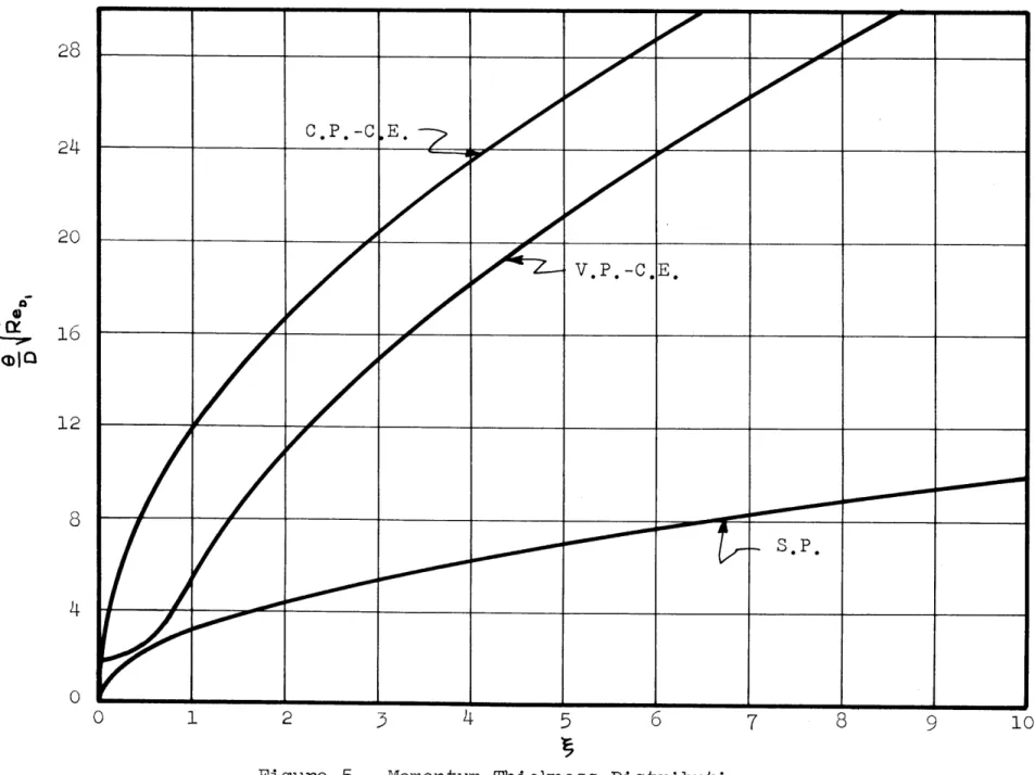
2,3 Momentum Thickness Distribution

In Ref, 6, Rott and Crabtree combine Thwaites' approxi-mate solution to incompressible boundary layers with the Illingworth-Stewartson transformation (Ref. 7), to obtain an explicit formula for the compressible momentum thickness in terms of the conditions at the edge of the boundary layer, Their derivation involves the previously stated assumptions of Prandtl number equal to unity and zero heat transfer at

10 1.0

.8-

-

- -

-

-

-

--

-

-.6

.4 0 0 2 4

6

8 10

3.2 2.8 2.24 1.6 1.6_ ____ __ 1.2 .8 .4 8- -_ __ _ _ _ __ _ _ __ _ _ __ _ _ 0 0 1 2 3 4 5 6 7 8 9 10

Figure 3 _{Isentropic Mach Number Distribution,}

0 10 20 30

Mach Number Distribution.

3.0 2.6 0 2.2

1.8

1.4 1.0 H 80 50 60 70 Figure 4

1t3

the surface, plus the assumption of a linear viscosity-temperature relationship. The expression for the momentum thickness & given by Rott and Crabtree may be

non-dimensionalized to yield:

Re

₌

.45

₍₎

6

_e

e e

where ₉₄₀₂

(2.2)

is a stagnation Reynolds number based on conditions at the singnation point,

Re,

*oz

For purposes of comparison, it will be desirable to express results in terms of the free stream stagnation Reynolds number

p

_Re

', P, D

-

_lto

The relationship between both stagnation Reynolds numberg using the fact that

7o T

may be found to be

.Po

Pe.,=e

- q

(T

*4

-

4

o r % _{= .6 2 Po}

(2.3)

Equation (2.3) becomes indeterminate at g 0 , an the stagnation point was therefore treated as follows:

d

From Fig.

3

point Me

it is evident that near the stagnation is directly proportional to 4 , There-fore, if

)

/S = constant

is small so that , and consequently *; equation (2.3) becomes / .672

(4-P0

DPOZ _~~

VI

j(~

5

_d~

/*4(5

Pa

= -

4P(

P

₂

/

/S may be found to have a value of 2.46 from Fig. 3 and therefore

[e~ I/;~

=1.70

₀

(2.4) and l. or and therefore

Re,,,---I

=O

15

Equations (2.3) and (2.4) are plotted in Figures 5 and 6 For the sharp and constant-pressure isentropic blunt plates, the boundary layer edge conditions do not depend on , and Eq. (2.3) may then be integrated to yield

frv

0 ~ (2.5)

for the sharp plate, and

(2,6)

C.PR-C.E. V P, T

for the constant-pressure blunt plate. These parabolic expressions for 0/, also appear plotted in Figures

5 and 6 ,

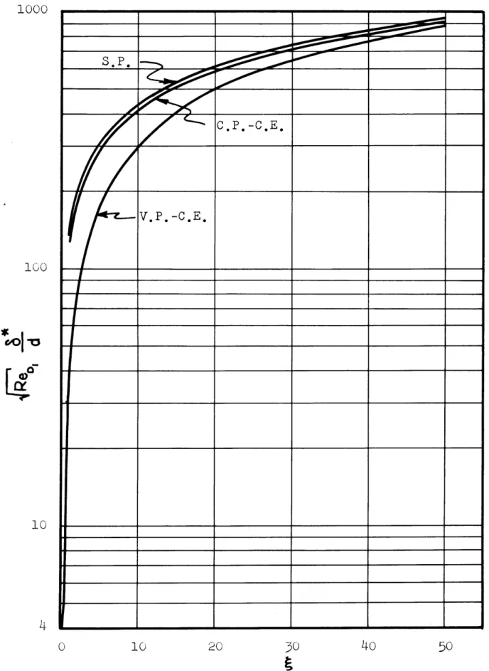
2,4 Displacement Thickness Distribution

Following Thwaites' method, the boundary layer

displacement thickness may be obtained from its momentum thickness by calculating the parameter m , which is related to the second derivative of the velocity distri-bution at the surface. The calculation of m will then yield another parameter

H

, which is the ratio of dis-placement to momentum thickness, Since Thwaites' results hold for incompressible boundary layers, it is necessary

28 20

20

V. P.-C E. 16 GIOI 12 4 0 _{Figu 5}

₇

₈

₉

₁₀

17

loole 1001 90 8o C.P.-C.3, V.P,-C.E. 70 600 50 4o 30 20 1457 -10 0 0 10 20 30 40 50 60 70 80

Momentum Thickness Distribution. Figure 6

18

to reduce the compressible parameter m to an

incompressible m. ; with this m. calculate the

in-compressible 14, ; and finally transform this I/' back to a compressible

The relationships between compressible and incom-pressible parameters are again given by Rott and Crabtree in Ref, 7. For rn, this is

dtlePox

2/T7e-Using the fact that

dUe

d

Me

-

ae

+

Me

d a

dx

_dy

_dx

the expression for m7 mfaY be written in terms of the

edge Mach number, the temperature ratio, a non-dimensional momentum thickness, and a grouping of terms which - not

sur prisingly - turns out to be the stagnation Reynolds

number Pe . Then writing Pe, _{in term s of} Pe,; m. becomes

19

Table I in Thwaites' paper (Ref. 5) will then yield

the incompressible parameter '6 . The compressible

1-may finally be obtained from a relationship given by Rott and Crabtree.

Te

7.er

(2.8)

Finally, the non-dimensional displacement thickness is obtained from

*

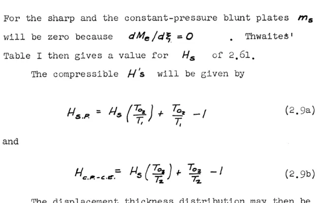
For the sharp and the constant-pressure blunt plates Ms will be zero because dMe

/di

= 0 . Thwaitet'

Table I then gives a value for

HS

and

of 2,61, The compressible #ls will be given by

-

(-~~

H

₅

7;

~-(2. 9a)

(2. 9b)

The displacement thickness distribution may then be obtained for these two cases by merely multiplying the momentum thickness distributions by the constant factors given by Eqs, (2,9a) and (2.9b),

20

1 2 2;

4

5

Displacement Thickness Distribution, 1000 100 10

4

0 FPigure 7

21

1000

10 20 ₃₀ 40 ₅₀

Figure 8 Displacement Thickness Distribution,

S

.

_ C.P,-C.E. V.P. -C.E. 100 10 24 0

The non-dimensionalized displacement thicknesses for all three cases appear in Figures 7 and 8

2.5 Boundary Layer Pressure Influence

As suggested in the introduction, the pressure correction due to the boundary layer is estimated by considering an inviscid body whose thickness has been increased by the displacement thickness, and estimating the pressure increment produced by a Prandtl-Meyer

expan-sion about this new inviscid body. Figure 9 illustrates this approach.

shock

plate

Figure 9

The local inviscid body inclination is assumed to be equal to the slope of the displacement thickness at the point of interest, and it is therefore necessary to obtain

2.

Since

-~-~~'

1

it follows that

v~7-d(

- _

+

-FoE,2/ From Eq. (2.) 7

_d(~/YZ

(P.72 /

z

r0 ~ZJ

7;~j

Ale

7 If OL7-) (2.11)

dA

03~

Expanding the derivative in the last term and collecting terms, (2.11) may be written as

v'~7

672

_(,

7 e a O

4

S

2

(r-z~j

Fzle

]?

~Te'

d~Te

(2.10)

(I

.1 (91Df Dj d

P-4

and substituting for

d

(9D

_re7, in (2.10), the final expression becomes

de

=

.9~

d_

.672

/

(

D1d- 4 g ft

(2.12)

Al

2 M_

dde

(

'V

C41

5 0 W 1L'

For the sharp and isentropic constant-pressure blunt plates, 1 and

Me

are constants and the terms involving their derivatives in Eq. (2.12) will drop out, The expression then reduces to

Si?

.336

for the sharp plate and

.336

- r- Y

M~~r.Z PaP( (2.14)

for the constant-pressure blunt plate.

Using the Prandtl-Meyer expansion approximation to calculate the pressure influence of the boundary layer, the non-dimensional pressure influence JP/pe is given to the first order by

(2.13)

X

J

d 'f

_{( J D}

T

25

Yle

d~

d({

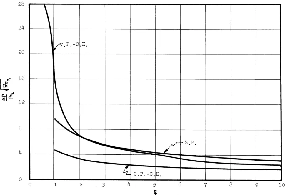
To provide a common reference for purposes of com-parison, it is desirable to evaluate the ratio AP/p, which is given by

Pe P0

po~

LpSPe]

(2.16)

For the sharp plate, Eq. (2.16) becomes

Pe,. &L5A

and for the constant-pressure blunt plate

fP)0L

M.7

-

)Y

__AD (2.18)

POL C.P-c.E

Equations (2.16), (2,17) and (2.18) may now be evaluated by using the corresponding expressions for _e

They are plotted in Figures 10 and 11

In order to evaluate the boundary layer pressure influence at the particular testing conditions for which experiments were carried out at the Aerophysics Laboratory,

28 24

v.P.-CE*

20 16 12

8

0 C P . -C E . O 1 2 34 56 ' 8 910O

Figure 10 Pressure Increment Distribution,

28 24 20

16

10 V* P. -C.E C.P. -C.E -- S P

35

Figure 11 Pressure Increment Distribution

R\) a~ 0 12

8

4

0 0

₅

₁₅ 20 25 30

F

it is necessary to calculate the free stream stagnation Reynolds number 1e., . The test conditions were

Al,= 7.6 = /z/T *oFbs.

/00pS/Cf. D= a/ in.

With these quantities, the free stream stagnation Reynolds number is found to have a value of

Re

=

951

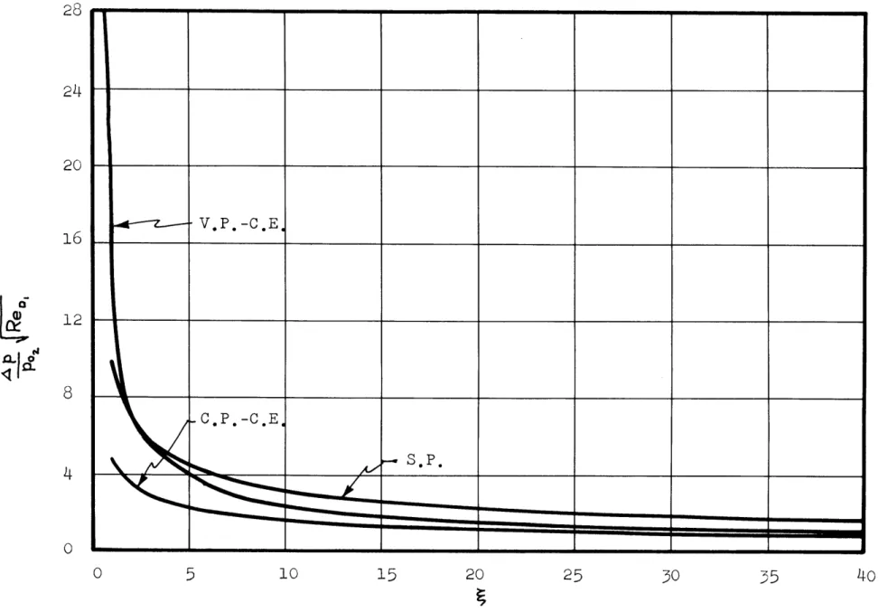
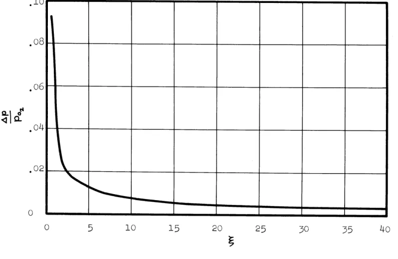
700

With this value of the Reynolds number the pressure dis-turbance for the blunt plate is plotted in Fig, 12 . It may be seen to be everywhere smaller than 10ox; and to become very small for values of greater than 7 or 8.

2.6 Discussion of Isentropic Results

Figures 5 and 6 show that the momentum thickness dis-tribution for the blunt plate may be closely approximated at the higher values of 4 by that for the constant-pressure blunt plate. The momentum thickness for the sharp plate is

seen to be considerably smaller than for the other two plates, over the entire range of ( , Figure 8 shows, however,

that at the higher values of , , all three displacement thickness distributions lie very close together, including the sharp plate di.splacement thickness. This may be explained

5 10 15 20 25 30

ro

-o

35 40

Figure 12 _{Boundary Layer Pressure Disturbance for M = 7.6,}

= _{95,700 on the Isentropic Blunt Plate.}

.1

0

0

by examining the transformation of the compressible H

for the sharp plate. This was

Since is greater than af or T0fy.

will be greater for the sharp plate than for the other two cases; this will tend to cancel out the effect of a smaller G/O and make the displacement thickness for the sharp plate roughly equivalent to that for the other two cases.

The calculations performed for the isentropic case have shown that it is possible to approximate the actual

blunt plate by a fictitious blunt plate with a constant surface static pressure equal to the free stream static pressure. Since the results show that this approximation becomes particularly good at large values of -which

is precisely the region wherenon-isentropic effects become important - the calculations suggest that it may be possible to replace the actual non-isentropic plate by a fictitious constant-pressure non-isentropic plate, and thus considerably simplify the solution of the non-isentropic case, Because the solution is simpler, the variable entropy case will be first solved under the assumption that the static pressure

free stream value. The complete variable-pressure, variable-entropy case will be solved last, and these more exact results will be compared to the simpler,

constant pressure approximations,

The calculations for the isentropic sharp plate

have provided an upper asymptote which the non-isentropic results should approach as the coordinate ' approaches infinity _.

312

CHAPTER ₃

DERIVATION OF PERTINENT BOUNDARY LAYER EQUATIONS

3.1 As discussed in Chapter 2, the boundary layer along

a blunt plate submerged in a hypersonic stream will have non-isentropic edge conditions. The static pressure will be assumed to vary as in the isentropic case, but the curved bow shock will produce a variation of stag-nation pressure which does not occur in the isentropic case. The non-isentropic edge conditions should approach isentropic values near the leading edge and far downstream from the leading edge.

The solution of the variable entropy problem differs from the solution of the isentropic case in two respects, First, the velocity at the edge of the boundary layer cannot be obtained directly from the static pressure dis-tribution, because Bernoulli's equation does not apply.

Secondly, Bernoulli's equation cannot be used in the solution or transformation of the boundary layer momentum equation,

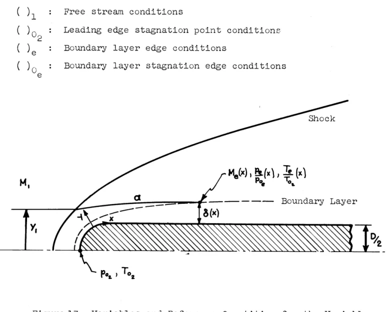
Figure 13 illustrates the pertinent variables and reference quantities for the variable entropy problem. Along the streamline a , the entropy is constant and stagnation conditions are therefore constant, If a shock

: Free stream conditions

: Leading edge stagnation point conditions

: Boundary layer edge conditions

: Boundary layer stagnation edge conditions

Shock

Boundary Layer

P. i To.

Figure 13 Variables and Reference Quantities for the Variable

Entropy _Problem.

(

)

()0 2 )e

(

)e MI

354

shape is assumed it is possible to obtain the stagnation conditions immediately behind the shock (at y,

)

because the local shock inclination angle will be known. These stagnation conditions will correspond to the edge stag-nation conditions at the point where the streamline er intersects the boundary layer, This discussion suggests that it is therefore possible to obtain the variation of boundary layer edge conditions with x by relating the streamline-shock intersection height

y,

to the spatial variable x

3,2 Energy Equation

The assumptions of Prandtl number equal to unity and zero heat transfer at the wall lead to a simple

expression for the temperature distribution in the boun-dary layer.

--

T

+ _/"

_M2

₂₍₃₁

Since at the surface of the plate the velocity is zero, the temperature

T

at the surface is simply given by

.

-

T

35

3,3 Momentum Integral

The purpose of integral methods is to reduce the

boundary layer continuity and momentum partial differential equations to total differential equations, by integration with respect to the y coordinate and the introduction of integral properties of the boundary layer, The bound-ary layer equations are

Continuity: _{Ip 3p) = 0 (3.3)}

dx _ay

Momentum: Ofu a"- +v U

'a_

__T+

A--

(

.4)

x

dx

ay

'ay

If the boundary layer thickness

c

is defined as the value of

y'

for which the velocity in the boundary layer is very close to the free stream velocity ("very close" meaning a ratio (u U,) of approximately _,999), Eq. (3.4) may be integrated with respect to

y

from

y=0

to

/=d

to give

8

a

u X

₀

_v

_y

0

d

-Y

_(3.

5

)

It should be noted that the last term on the right-hand side of (3.5) involves the assumption that

36

This is not strictly true, because the entropy gradient normal to the surface will produce an inviscid velocity gradient. However, as mentioned in Chapter I, the Reynolds number considered is high enough to permit the assumption that

f

Jef

IY y=8 D)'

y=O

and consequent neglect of the inviscid velocity gradient compared to the viscous velocity gradient.

After some algebraic manipulation described in detail in Appendix A, the boundary layer momentum equation may be written as

dx

dx

d

~

where G: momentum thickness 3 : displacement thickness

thickness

which is the integrated momentum equation, and which will reduce to the Karman momentum integral for the isentropic case, where

From (3.4), since at y - 0 ; u=O, v=O

3,4 Transformation of Momentum Integral

In subsequent work, use will be made of the relation-ship found by Thwaites5 between the first and second

derivatives of the velocity at the surface, and the ratio of displacement to momentum thickness, Since Thwaites' results hold for incompressible boundary layers, it is

necessary to find some relationship between the compressible boundary layer variables and those of an equivalent incom-pressible boundary layer, This is accomplished, following Hammitt , by the use of the Howarth transformation,

which replaces the coordinate y by a coordinate

S

such that

dy

.--

d

Te

In that case,

eP

|_ ue IPT

,

P

f_

T

U

o

Pee

38

and since

T=

/

r te

where the subscript6

(3.8)

d_

=s

.ged

denotes incompressible variables, Also,

dy

(3.9)

-

_e

and 0 Substituting for (t-T) T a e

C/5

(3.10)

in (3.10) from the energy equation

17/

-z

UZ)7d5

Cez

<U

/

(6

₊

(s '

e

S

=f

0

I

+2 S (/-or =- + _e CS

_{= CIS}

(;--

a*

-

(U

d6OI *311

F

dS 37Ys=Q 0 T e s

-

o

T

The transformed momentum equation and boundary con-dition will therefore become

+ z Te

and

dpe

(dS

/sro

3.5 Thwaites' Results for Incompressible Boundary Layers A brief discussion of Thwaites' approximate solution

for incompressible boundary layers with arbitrary pressure gradients is presented in this section. Thwaites' approach

39

The first and second derivatives of the velocity at the surface are transformed as follows:

and

(3.12)

2yzy.

_(3,13)

(3.15)

r

₄₀

is then used to derive a method for obtaining the dis-tribution of a new boundary layer parameter needed in the solution of the non-isentropic equations,

In Ref. 5, Thwaites attempts to find some universal relationship between the first and second derivatives of the velocity at the surface for one-parameter families of solutions. He defines non-dimensional parameters

/sd

0. S (3.16a) (3.16b) (',16c) s

-The parameter M₅ is related to the pressure gradient through the boundary condition at the surface, and it may therefore be determined if this pressure gradient is known, Thwaites then proceeds to plot the parameters is and A/I

as functions of r, for several special forms of the pressure gradient, for which the boundary layer equations have been solved exactly. He notes that these curves lie

fairly close together, particularly for the case of negative pressure gradients (negative /s ). By fitting the best

average curve to the s -m, and /-/ - m. plots for the different exact solutions, he finds a fairly universal relationship between these parameters, which he presents in

41

tabular form in Table I of his paper. For the solution of an isentropic boundary layer (for which Bernoulli's equation may be used), a combination of the previous parameters in the form

LSe - 2

[(S+2).

7+

(31

()]

is important, and Thwaites shows that the parameter lies within close limits for all the exact solutions throughout the entire range of ms , Furthermore, the average variation of

L.

with ms is very close to

linear, and Thwaites then assumes a universal relationship.

L,=

.4sj-

6rm (3.18)

With Thwaites' definitions of the incompressible para-meters, Eqs. (3.12) and (3.13) may be written as

d

_U,

_9. dx J dPT74L7e- (35.19) and _ s (3,20) z

42

As will be seen later, a new non-dimensional parameter appears in the solution of the non-isentropic case. This is the difference between boundary layer and displacement thicknesses, divided by the momentum thickness. This parameter has been shown in Section 3.4 to be independent of the coordinate transformation, That is,

K -s

It is desirable to obtain some relationship between this parameter Ks ahd the parameter ,n , This has been

done following an approach analogous to Thwaites', k

*

was plotted as a function of M. for three know cases The Faulkner-Skan1 1 solution, the Karman-Pohlhausen8

solution and the Howarth8 solution for pressure gradients of the form

P.

= a +/bX' . The results appear plotted

in Figure 14 , It may be seen that they lie fairly close together. From Figure 14 , a simple linear "universal" relationship was fitted:

K

, -. 60 m e h6.2 (3.21)

KS -10 Faulkne: -Skan

8

Assumed "Uiiversa]" Howart Karman- ohlhaus an 4z: -.10 -.08 -.06 -.04 -.02 0 .02 .04 .o6 ms s .08 1.0 Variation of Ks with _{m .} Figure 1 4_

44

3.6 Shock-Boundary Layer Continuity Equation

In Section 3,1 it was suggested that the variation in boundary layer edge conditions with x could be obtained by relating x to the height y, at which the streamline intersecting the edge of the boundary layer at x intersects the curved shock, This may be done by writing a mass-balance equation between a station

ahead of the shock and a station at X (see sketch in Figure 13), Since the mass flow in the boundary layer

is equal to A Ue (f- 0) , this relationship will be - for unit length along the span

Ap,iY,

<660*)e Ue

or

jol e U 1< ' = Oe(3,22)

3.7 Shock Shape

As stated in the Introduction, a hyperbolic shock shape following the results of Love (Ref. 3) has been assumed. Figure 15 illustrates the important variables and parameters in Love's damplified calculation of the shock shape. Figure 15 is a reproduction of Figure 9 in Love's paper, with some of the letters changed to avoid confusion with other variables being used in the present discussion,

45

Asymptote

Hyperbolic Shock

Sonic Point _{Control Line} on Shock

es

0

d' :Diameter at which body has a slope equal to tan _{S det}

6_{det Angle at which shock detachment first occurs}

for _{a wedge in a stream at M1} : _{Mach angle corresponding to M}

es

Angle at which the Mach number behind the shock is equal to unity

Local shock inclination angle

46

The assumption of a hyperbolic shock shape which is asymptotic to a Mach line yields an expression of the form

It is necessary to evaluate the quantity ,/D) which for semicircular noses is related to (Yo/d) by

0 = 0.* c (3.24)

D

d' det.

Love evaluates the quantity (X0

/d')

by a method which

is essentially based on a large number of experimental results obtained at different Mach numbers, He presents an empirical graph of the inclination angle o( of a "control line" which is representative of, though not equal to, the sonic line. He then uses trigonometric relationships derived by Moeckel, to relate oc to the quantity (x₀

/d)

. The relationship is

\|, - '(M,-)tan~e 5 / [ + ( .25)

47

where (x'/d') is the shock-standoff distance, which Love assumes to be simply given by

. det. _(=o.26)

The coefficient C is also obtained from experi-mental results, It will be equal to unity if the shock is attached, and have a value close to unity when the shock is detached, Love's Figure 2 gives the variation of this coefficient with free stream Mach number,

For the purposes of the present analysis, it will be useful to relate the coordinate y, to the local

shock inclination angle . This may be done as follows: From Eq. (3.23)

dyi

tan,

Solving for X,/D

(A=-)tanp

-9

48

for

4

tan~f

I

_'"/ _

/

(,3.27)

-H

(H :--!)(y

For the particular free-stream Mach number being con-sidered (Hl, =

7.6),

det. = 430

Mfz-I =56.76

C

4

t and e have been obtained from the NACA

isen-tropic flow charts and tables (Ref. 10)).

Love's Figure 2 yields a numerical value for

C

of .951, at Al, = 7.6. (X'/d) may therefore be calculated. In orderto obtain a , it was necessary to extrapolate Love's graph for the experimental variation of a with

M/, This extrapolated distribution is shown in Fig, 16.

a

for = 7, 7.6 is then found to have a numerical value of 76.5 . (xo/d') may then be evaluated, and finally (1/D) may be found to have a value of 57.3. Substituting then into (3.25), the expression for 9 becomes

49

1 2 3

4

5

6

7

8

Figure 16 Variation of c with M .

80

70

6o

50 4o 30 20 10 0

50

CHAPTER 4

CONSTANT PRESSURE-VARIABLE ENTROPY CASE

4.1 The results described in Chapter 2 have pointed out the possibility of replacing the actual isentropic blunt plate by:.a fictitious isentropic plate with constant static pressure. The results in both cases were shown to be

approximately equivalent, especially at the higher values of t , This approximation will now be carried into the non-isentropic region, because the assumption of constant static pressure considerably simplifies the analysis. For the constant-pressure, variable-entropy (C.P.-V.E.) case, therefore,

dx

This means that the Thwaites parameter n. will therefore be zero everywhere. All other parameters which are functions of m , i.e.,

1

, and

k

, will therefore remain

constant at the values corresponding to n 0 . It should be noted, however, that since Bernoulli's equation

51

no longer applies, dUe/dX will in general not be equal to zero.

4.2 Solution of Momentum Equation

For constant static pressure, the transformed momentum equation (3.19) will reduce to

~~20 )

d~~~~~

p

4

e

(Ze~

<44

d6 T

(4.

_*

1)

dx

e (

AO

and the boundary condition at the surface yields

d p, /V T e1 ,

dx

~(T)

or

MS=

These equations hold, of course, under the assumptions of and qf = O for which (3.19) was derived, Equation (4,1) will be solved using the shock-boundary layer continuity condition (3,22) to obtain a relationship

between

f,

and the boundary layer edge conditions. Equation (3.22) may be written

K S

52

KS dx d 1

Multiplying through by 2 Ks AU, derivative,

and expanding the first

12

U

_{2U_}

,

4' +2(f - A<, , 2 /<e e

-

gU

_S

7

dIX dx t?,U, 'g&

and multiplying through by

(y,

/

due

Ue C/X S

,(.la

(4.1a)

-/

(4.2)

using the iso-energetic flow equation for the temperature ratio, Taking the logarithm of both sides, (4.2) becomes

2 / Un ao = 2

z

sdx

Now

53

Differentiating implicity and collecting terms,

Ne_ / +Mz

Substituting into (4.Ja).,

-.I z 2

-OgU p U "/o

where _{j - 1D} has been substituted for x

The right-hand side of Eq. (4.3) may be modified to simplify calculations as follows:

2 1s ks

a, P,

Re Me. 7

V|( 4 .3 a )

[_ 2 s s

where

Rep?

= (aC42o A is the stagnation Reynolds

number based on conditions at the nose of the plate.

The bracketed quantity in (4.34 will be a constant for any given free-stream conditions, and will be denoted by B Equation (4.3) may therefore be written as

d

/2 _{(Y 2.(/- s) df} -

B

Me(7 0_z

(4.4)

_ dUe _ edu d4 *d (4.3) , Pe,

p,1

M, aj p, M, a, o 07 Tj z _{;;I_) (7, TO-2}

54

Equation (4.4) is an ordinary first order differential equation in the variable

which are functions of

Y ( 7 2 , with coefficients . It may be solved exactly, and the solution (Ref. 12) is given by

f)P(e)d

0

-

int/ cons

/an/

(4.5)

where

Xj/)

P(4)

Q(4)

= 2(/ -ks) de Me(/#lie _d$ = BMZ

The integration constant will be zero because

7(0)

=

0

Carrying out the integration of P{(,) to obtain that

P(u)d

= (-) /n{

Equation

(4.5)

then becomes

, it is possible

[To

_{I O}

meZ

_- ( i- )

Tor

/12.

55

(k-)

-Z3-z1,

eO

Me '

2

d{

(4.6)

0

With given boundary layer edge conditions, Eq, (4.6) yields the shock intersection point of streamlines

inter-secting the boundary layer at J() , By assuming an edge Mach number distribution, it is then possible to calculate the shock intersection parameter

7

as a function of ' , With the assumed hyperbolic shock

shape it is then possible to obtain the local shock inclination angle d as a function of , , (See Fig. 17.)

56

Using oblique shock relationships the stagnation pressure behind the shock can be obtained, which is equal

to the local edge stagnation pressure boe , aat , The ratio Pe/p,, will then yield a new edge Mach number distribution through the isentropic relationship between pressure ratio and Mach number

Y

This isentropic relationship may be used in this case because the entropy along the streamline in Fig, 17 is constant, With the new edge Mach number distribution, a new 7, may be calculated by using Eq, (4,6), and the iterative procedure may be continued until the edge conditions converge to some final distribution,

When the final edge conditions have been calculated,

the momentum thickness may be obtained from the shock-boundary layer mass balance equation, which has been seen to be

(4.7)

From the momentum thickness, the displacement thickness and displacement thickness slopes may be calculated; and finally, the boundary layer pressure influence coefficient

57

4.3 Calculations and Results

4.3.1 Calculation of Edge Conditions

The constants in Eq, (4.6) must be evaluated before proceeding with calculations. The constant

is computed from the Blasius solution to the flat-plate problem, and is found to have a numerical value of 6.43, Table .f in Ref, 8 has been used, choosing as 3 the point where

(./Ue)

= ,99898. The constant

B

has been calculated from the NACA Compressible Flow Tables

(Ref. 10) and is found to have a numerical value of 1,837 x 10~

,

Equation (4.6) then becomes

1g9 I -4.9I

/.3 M4fM1 _{0 /Z 0'1 (4.8)}

For the first iteration the edge conditions are assumed to be those for the isentropic case, i.e.,

Me = 3.4868 = constant

A value

(O)

= 6.43 from the Blasius solution was assumed rather than the value given by the "universal" relationship K5 - /.6rm,+6.2 , because the Blasius

58

Once has been calculated from Eq. (4.8), the shock inclination angle > at

>

can be obtained from Eq. (3.28). Three distributions of were cal-culated following the iterative scheme described above and the results are shown in Figure 18, # lies close enough to so that it was not necessary to compute any further approximations. The final shock angle distri-bution /3 yields the final edge Mach number distri-bution Me , which is shown in Figure 19, together with the Mach number distributions found for the other iterations. It is evident that the edge Mach number varies between the isentropic constant-pressure (C.P.-C.E.) value of 3.487, and the free stream value of 7.6.

4,3,2 Calculation of Momentum Thickness With the final edge Mach number distribution Eq. (4.7), transformed to

V

T~c-(4,9)

where

C

= - = 4/87:3

was used to compute the momentum thickness distribution which appears in Fig. 20. In Fig. 20, the momentum thickness is seen to vary between those of an isentropic constant pressure blunt plate (C.P.-C.E.) and the isentropic, sharp plate (S.P.)

50

20

0

101 102

Shock Inclination Angle at

58 --- -- m - ---

-I(2

4 d ---- - - - - --

---i--M

Figre9 Ed020 ₁₀

101 10 101

7 7

I luo10

Op

00

C -P Oloop 00 I 001, #00, 1000' 000, -100 00000 0000P 00 00 I-C.PI.-V.,E.I l/ 000P -,00 al '0 100 ,Ow-OOOOp- 00 1 00010 000 102

Figure 20 Distribution of Momentum Thickness,

H

62

4.3.3 Calculation of Displacement Thickness For the non-dimensional incompressible case, the displacement thickness is given by - following Thwaites5

*o D

where can be obtained from Thwaites' Table I. For the case of Ms = O , which corresponds to the constant static pressure assumption, / has a numerical value of 2.61.

The compressible displacement thickness may be obtained from a similar expression

(*2/

-D

P)

(4.10)

provided an equivalence between the compressible parameter 1' and the incompressible parameter can be found. This relationship is obtained as follows:

By definition, the compressible displacement thickness

is given by

(

- _{_./ )dy}

o

PeUe

r

with the Howarth transformation

dy= dS

T

4~

(T 6)

)

dS

From the energy equation for the case of and zero heat transfer at the surface,

_T = / + z / -2

Substituting into Eq. (4.11), collecting terms and using the definitions for the incompressible momentum and displacement thicknesses,

6*::

C~5 4 Y_/M2 2 le (Gs 4 s/ or, since 0 , ~ 2 / (4.12)

Writing Eq. (4.12) in terms of the temperature ratio, the non-dimensional compressible displacement thickness will finally be given by

~~DI Z M4l

0

D

(4.11)

64

With the edge conditions given by M( in Fig, 19, Eq. (4.13) has been plotted in Fig. 21. The values of

for the sharp and constant-pressure isentropic flat plates are also displayed in Fig. 21 for purposes of comparison.

4.3.4 Calculation of Displacement Thickness Slope

From Eq. (4.10), the non-dimensional displacement slope is given by L5 (4.14) where _e (4.14a) + Z (4.14b)

The differential terms in Eq. (4.14) will be transformed until they appear as a function of a single derivative - the edge Mach number slope.

From Eq. (4.14a),

Zm / __

d'e

d

2 He (4.15)

The derivative in the last term of (4.15) may be written as

d(T 7)

_ _

dM*+

2

7

1021 D10i 10

Figure 21 _{Displacement Thickness Distribution.}

100

*

10

ol

r

66

and substituting for from Eq, (4.4),

( T2 32

d

7db

de

(0 Combining terms,

dr(=

e 2 dMe 7

7

d(7N

/cr zAle dL e

Substituting in (4.15) and combining terms,

dj%)

cB

(

T 2/

dle

(

2T M Ale dTo

r

7e- (4.16)

From Eq, (4.14b),

(4.17)

and substituting (4.16) and (4.17) into (4.14),

___

CI

/7~'

/

/1

d~le

(9

d(002

(2"IDd

02

Mie('%9

M

dj

d

and collecting _terms

d(

J/o) = C21 A/ Te

(12s)

1dA1e

Tz Me L1D To 'a

OZ Ta(4.18)

Equation (4.18) has been plotted in Figure 22, The edge Mach number slope was calculated by drawing a large-scale graph of the edge Mach number distribution and fitting tangent lines at the points of interest, The displacement thickness slopes for the two isentropic plates are also displayed in Fig. 22,

4,3,5 Calculation of the Pressure Influence of the Boundary Layer

In order to calculate the pressure increment produced by the presence of the boundary layer, a Prandtl-Meyer

ex-pansion about an effective inviscid body whose local surface slope is equal to the local slope of the displacement thick-ness is assumed, The expression for the pressure disturbance will then be, to the first order,

10-1

10

-0C'

10

10 10 2 13 10 4105