How does ocean ventilation change under global warming?

(1)

HAL Id: hal-00298399

https://hal.archives-ouvertes.fr/hal-00298399

Submitted on 11 Jul 2006

HAL is a multi-disciplinary open access

archive for the deposit and dissemination of sci-entific research documents, whether they are pub-lished or not. The documents may come from teaching and research institutions in France or abroad, or from public or private research centers.

L’archive ouverte pluridisciplinaire HAL, est destinée au dépôt et à la diffusion de documents scientifiques de niveau recherche, publiés ou non, émanant des établissements d’enseignement et de recherche français ou étrangers, des laboratoires publics ou privés.

How does ocean ventilation change under global

warming?

A. Gnanadesikan, J. L. Russell, F. Zeng

To cite this version:

A. Gnanadesikan, J. L. Russell, F. Zeng. How does ocean ventilation change under global warming?. Ocean Science Discussions, European Geosciences Union, 2006, 3 (4), pp.805-826. �hal-00298399�

(2)

OSD

3, 805–826, 2006 Ventilation under global warming A. Gnanadesikan et al. Title Page Abstract Introduction Conclusions References Tables Figures J I J I Back Close Full Screen / Esc

Printer-friendly Version Interactive Discussion

EGU

Ocean Sci. Discuss., 3, 805–826, 2006 www.ocean-sci-discuss.net/3/805/2006/ © Author(s) 2006. This work is licensed under a Creative Commons License.

Ocean Science Discussions

Papers published in Ocean Science Discussions are under open-access review for the journal Ocean Science

How does ocean ventilation change under

global warming?

A. Gnanadesikan1, J. L. Russell2, and F. Zeng3 1

NOAA Geophysical Fluid Dynamics Laboratory, Princeton, NJ, USA

2

Department of Geosciences, University of Arizona, Tucson, AZ, USA

3

RSIS, Princeton, NJ, USA

Received: 29 May 2006 – Accepted: 19 June 2006 – Published: 11 July 2006 Correspondence to: A. Gnanadesikan (anand.gnanadesikan@noaa.gov)

(3)

OSD

EGU

Abstract

Since the upper ocean takes up much of the heat added to the earth system by an-thropogenic global warming, one would expect that global warming would lead to an increase in stratification and a decrease in the ventilation of the ocean interior. How-ever, multiple simulations in global coupled climate models using an ideal age tracer

5

which is set to zero in the mixed layer and ages at 1 yr/yr outside this layer show that the intermediate depths in the low latitudes become younger under global warming. This paper reconciles these apparently contradictory trends, showing that a decrease in upwelling of old water from below is responsible for the change. Implications for global biological cycling are considered.

10

1 Introduction

The rate at which the interior ocean is ventilated by young surface waters has an im-portant impact on many imim-portant elemental cycles. The distribution of oxygen, for example, is controlled by a balance between supply from recently ventilated waters and consumption due to remineralization of organic matter. Large oxygen minimum

15

zones at intermediate depths can be found where the ventilation is comparatively slow (Fig.1a). Since the oxygen minimum zones are regions where the critical nutrient ni-trate is consumed (Gruber and Sarmiento,1997) changes in the oxygen distribution can have important effects on the nitrogen cycle and in the production of radiatively important trace gasses such as nitrous oxide (Elkins et al.,1978;Wallman,2003).

Al-20

tabet et al. (1999) suggested that large changes in nitrogen isotopic composition of sediments over the past million years resulted from changes in the size and intensity of these minimum zones. Galbraith et al.(2004) recently revisited this hypothesis using a number of cores from around the world and found evidence for global scale changes in ventilation rates.

25

(4)

OSD

EGU

important to understand how the ventilation of these zones may change under global warming. Because global warming is expected to add heat to the upper ocean and such heating would be expected to increase the overall stratification and make it harder to mix into the interior (see for example Sarmiento et al., 2004) one would in general expect the ocean interior to become older. Additionally, the slowing of the Walker

5

circulation (Vecchi et al.,2006) would also be expected to reduce tropical ventilation. However, the increase of the hydrological cycle is expected to make the tropics more salty, which might, in some regions, compensate this effect. Finally, changes in the distribution of winds, particularly in the Southern Ocean (Russell et al., 2006) may also act to increase the rate of ventilation.

10

A number of global coupled climate models, including three developed at the Geo-physical Fluid Dynamics Laboratory (GFDL) have included a tracer of ventilation age known as the ideal age. This tracer is set to zero in the mixed layer and ages at a rate of 1 yr/yr thereafter. In this paper, we examine simulations using this tracer and find the surprising result that one of the most significant changes in ideal age under

15

global warming is that the regions where oxygen is currently at low levels become younger. The reasons for such a change are examined in one model for which full term balances are available and are attributed to a decrease in the upwelling of older intermediate waters from below. Implications of this result for global biogeochemical cycles are considered.

20

2 Description of the simulations

Two model configurations are primarily used in this paper. These are the GFDL’s CM2.0 and CM2.1 models developed for the Intergovernmental Panel on Climate Change Fourth Assessment Report (IPCC AR4). The CM2.0 model is run using the new B-grid atmosphere described in GAMDT (2004) with a 50-level ocean model based on

25

the MOM4 code base ofGriffies et al.(2003). The CM2.1 model is run using the same atmospheric column physics as CM2.0 but with a finite-volume core (Lin,2004) which

(5)

OSD

EGU

produces a significant poleward shift in the winds, particularly in the Southern Hemi-sphere leading to significant improvements in the ocean simulation (Gnanadesikan et

al., 2006). More details on the ocean model formulation are given in Griffies et al.

(2005). The models are run without flux adjustments. The control climate simulations are described inDelworth et al.(2006). and simulations under idealized climate change

5

are described inStouffer et al.(2006).

The initialization procedure is based on Stouffer et al. (2004). The atmospheric model is initially run for 17 years with observed sea surface temperatures and sea ice. The resulting heat and water fluxes and observed wind stresses were used to run an ocean model initialized with temperatures and salinities from the World Ocean

10

Atlas (2001) for one year. The restart files from these two runs were used to initialize a “1990 control” in which radiative forcings were held constant at 1990 values (years 65– 70 of this control run are used to compare with CFC-derived ages). “1860 Control” runs are generated from year 21 of the 1990 Control by setting greenhouse gasses to 1860 conditions and allowing the model to adjust for some period of time (300 years

15

for CM2.0, 220 years for CM2.1). The final restart files from these spinup runs are then used to initialize 1860 Control runs and a number of climate change scenarios. We will focus on the idealized climate change scenario reported inStouffer et al.(2006) where the CO2 is allowed to increase at a rate of 1%/year until it doubles 70 years after the initial run. After this point the CO₂is held constant. The majority of the results compare

20

the second century of the control run with the second century of the doubled CO₂run. In order to examine the robustness of our results, we also use the R30 global cou-pled climate model which was developed at GFDL for the Third Assessment Report of the IPCC as described inDelworth et al.(2002). In the R30 simulations, the ocean circulation is run out to steady state before the model is coupled to the atmosphere, so

25

that the ideal age is essentially at steady state in the ocean. It thus provides a mea-sure of how much our results may be biased by the fact that the age is not at steady state as well as providing a third simulation with a significantly different atmosphere and ocean. The R30 model has a spectral atmospheric core at R30 resolution

(6)

(nomi-OSD

EGU

nally 3.75◦by 2.25◦) and a 19-level, 2 degree ocean developed using the MOM1.1 code ofPacanowski et al.(1991). This model does not contain many of the more modern physical parameterizations found in the CM2 series such as an explicit mixed layer and the eddy-induced advection parameterization ofGent and McWilliams(1990). The R30 model was run with flux adjustments so as to prevent the ocean from drifting too far

5

from the present state.

3 Results

The oxygen minimum zones reflect the underlying dynamics of the ocean circulation. At many depths and along many isopycnals, clear plumes of oxygen-rich water emanate from the eastern polar corners of the basins and seem to follow the gyre circulation

10

into the interior. In the southeast Pacific, for example, Reid (1985) showed that the boundary between low oxygen and high oxygen zones at mid-depths corresponds to boundaries in steric height corresponding to boundaries between flow rapidly ventilated from the south and more sluggish closed circulations or even flow from the north.

The ventilated thermocline theory of Luyten et al. (1983, henceforth LPS) suggests

15

that such a boundary should exist as a result of potential vorticity (PV) dynamics. Be-cause eastern boundaries cannot provide the friction to allow parcels to change their potential vorticity f/H, geostrophic flow right at the boundary will be sluggish. Instead boundary waves act to homogenize H, removing pressure gradients and resulting in north-south potential vorticity gradients which act to block the gyre flow. The resulting

20

shadow zones have small values of PV which cannot connect directly to larger values found in outcrop regions of mode and intermediate waters. As a result, these regions cannot be directly ventilated by time-mean geostrophic flows and will be older than the ventilated interior gyre. The LPS theory does not predict the age of the shadow zones, since the processes responsible (diapycnal and isopycnal mixing) are not included.

25

Observations of the density structure and CFC-12 age (Fig.1b) show that the oxy-gen minimum zone does in fact correspond to a strong gradient in both CFC age and

(7)

OSD

EGU

potential vorticity as suggested by LPS. The coupled models (Figs.1c, d) are able to reproduce the potential vorticity gradient, and have a significant gradient in ideal age at this point as well. Note that CFC-12 age (computed by taking the date at which the CFC12 in the water would have been in equilibrium with the atmosphere) is not strictly comparable to the ideal age due to the fact that it will be biased high by lack of

5

equilibration in sinking waterRussell and Dickson (2003), and biased low by mixing. Qualitatively though, the CFC ages range between 35 and 50 years in the shadow zones, while the ideal age is around 45 years, suggesting that the ventilation in the models is roughly comparable to the observations.

Under global warming, the ideal age in these regions change significantly. Figure2

10

shows the ideal age changes in the three GCMs at 300 and 800 m. In the high latitude Southern Ocean and North Pacific, global warming produces an increase in ideal age, as increasing stratification slows the rate of ventilation. However, in the tropics, the ideal age actually decreases over a wide range of latitudes, with some of the largest differences seen in the shadow zones. The differences are largest in the R30 model.

15

The CM2.1 model has the smallest changes at 300 m while the CM2.0 model has the smallest changes at 800 m. Note that the models differ significantly as to whether the South Pacific will get older or younger under global warming, with the R30 model suggesting that it would become older and the CM2.1 projecting a significant decrease in ideal age. Differences are also seen in the extent to which Northern Indian Ocean

20

becomes younger, with the CM2.1 and R30 models suggesting that this region will become younger, while CM2.0 suggests relatively little change. All three models do show decreases in age in the shadow zones, particularly in the North Pacific.

The age decreases at intermediate depths contrast with age increases in the deep, as shown by zonally-averaged ideal age change in Fig.3. All three models show the

25

tropics becoming younger above depths of 2000 m, with larger increases below this depth. When horizontal averages are taken, it can be seen that the average increase in deep ideal age is between 20 and 50 years, with the largest values being found in the R30 model. At shallower depths, the age may actually decrease in the horizontal

(8)

OSD

EGU

average, depending on whether the increase in ideal age in the subpolar regions is sufficient to cancel out the decrease in ideal age in the tropics. Although the magnitude of the age changes are much bigger in the R30 model, the broad similarity of the three patterns of ideal age change suggests that the basic pattern of change is not merely a function of details such as whether the model is flux-adjusted or whether the model at

5

equilibrium (in both cases the R30 model is while CM2 models are not).

Recent work (Russell et al., 2006) has shown that one can estimate the uptake of anthropogenic carbon dioxide by examining the ideal age distribution. As the bulk of the anthropogenic transient has occurred in the past 50 years, the bulk of the carbon is contained in water that is relatively young – the rapidly-ventilated subtropical gyres and

10

recently ventilated deep waters. The volume of this “young” water thus constitutes an interesting diagnostic of model evolution. Figure4shows the volume of water younger than 50 years in the CM2 series. The CM2.0 control run has less young water than the CM2.1 control run (145.2 vs. 152 Mkm3), a difference of about 4%. Under global warm-ing the volume of young water decreases with high latitude Southern Ocean ventilation

15

and Northern Hemisphere ventilation declining in both models. However, the volume of young water in the mid-latitudes of the Southern Hemisphere actually increases under global warming in CM2.1 and holds essentially constant in CM2.0.Russell et al.(2006) argue that this increase can be attributed to the poleward shift of the Southern Hemi-sphere westerly winds found under global warming. This region is important, since on

20

short time scales most of the anthropogenic carbon taken up by the ocean ends up in these relatively young waters.

The changes resulting from global warming are striking in part because they occur in regions where the variability is relatively low. Figure 5 shows time series of ideal age at 300 m in four regions, the Eastern Tropical North Pacific (5 N–15 N, 150 W–90 W) which

25

includes the core of the northern shadow zone, the subpolar North Pacific (45 N–55 N, 150 E–150 W), a region including the Peru Current and offshore waters (10 S–25 S, 100 W–70 W) and the southern ocean (65 S–55 S). Note that CM2.1 is younger than CM2.0 at this depth throughout the world ocean, reflecting in part the difference in the

(9)

OSD

EGU

initial spinup. All the control simulations show clear trends in the early, and in some cases the later part of the record as well, reflecting the spinup of the age field. In the two shadow zone regions, there is a very clear separation between the global warming cases and the control cases, with the variability occurring on very short time scales (2–5 years) and much smaller than the signal. At or near the time of CO2 doubling the

5

shadow zones have begun to become clearly younger. Doubling carbon dioxide alone corresponds to a radiative forcing of 3.7 W/m2. This is only about 25% larger than the 2.8 W/m2that is seen today in our models (T. Knutson, personal communication). By contrast in the subpolar regions, the variability is of the same order of magnitude as the net change.

10

4 Discussion

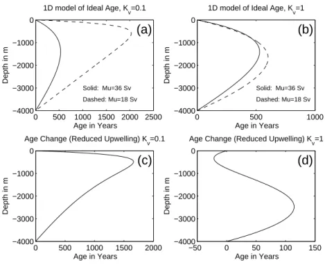
Insight into the reasons for the change in the ideal age can be gained by considering a one-dimensional advective-diffusive model. In this model young water is injected at the base of the domain (z=−D) and upwells through the thermocline, aging as it does so. Additionally, young water is mixed down from above. The equations governing the

15

age A in such a system are

∂A ∂t = −w ∂A ∂z + ∂ ∂zKv ∂A ∂z (1a) A= 0 z = 0, −D (1b)

Where w is the upwelling velocity, and Kv is the diffusion coefficient. These equations yield an equilibrium solution

20 A= 1 w z+ D(1 − ezw/Kv₎ 1 − e−wD/Kv ! (2)

This solution has two regimes. When wD/K_vis large, the primary balance over most of the domain is between the advection and aging. As upwelling decreases, the age

(10)

OSD

EGU

increases throughout the column (Fig.6a). When wD/K_v is small, on the other hand, the balance is between the diffusion and the aging and the advection has little impact on the total age, only moving the location of the maximum. Under such a regime (Fig.6b) reducing the upwelling decreases the age in the surface and increases it at a depth, a profile strikingly similar to those seen in Fig.3d. This does not mean necessarily that

5

diffusion is important in the model, since the diffusive coefficient is actually quite small. Instead, it means that the primary source of younger water is from above, as a result of wind-driven advection rather than from below as a result of diffusively driven advection. Practically, this would imply that the mechanism for the age change is a decrease in the supply of old water from below.

10

Such a picture is supported by Fig. 7, which shows the budget of ideal age from years 220 to 240 of the 2X and 1860 control runs. The diffusive transport of age (encompassing both vertical diffusion, convection, and the vertical transport associated with eddies) hardly changes at all between the two simulations (Fig.7c). Instead, we see a large change in the upward advective flux of age below a depth of 1000 m (above

15

this depth the advective flux of age actually increases somewhat). This is consistent with a spin-down in the overturning circulation (Fig. 8) which is seen in all three models. As a result the age in the intermediate waters drops (less old water is being injected from below) and that at depth increases (less old water is being exported vertically). This explains in part why the signature of global warming on ideal age is so much

20

larger in the R30 model. In the R30 model (which is at equilibrium) ideal ages in the deep ocean are very high. Reducing the upwelling of this old water produces a much bigger signal than in the CM2 series. An additional reason for the difference between the models is that the magnitude of the overturning changes differs between the models. The CM2.0 model has very little deep convection in the Southern Ocean

25

(Gnanadesikan et al., 2006) and little formation of Labrador Sea Water. As a result, when the planet warms, and these regions restratify the overturning changes relatively little. By contrast, in CM2.1, the Labrador Sea actually cools under global warming as convection in this region shuts off (Stouffer et al.,2006). The R30 model has an even

(11)

OSD

EGU

larger decrease in the overturning, further enhancing the increase in age at depth and decrease at age in the intermediate waters.

5 Conclusions

We have shown that under global warming, the ocean shadow zones may become younger, as less old water from below upwells into these regions. This result appears

5

to be robust across three models that differ significantly in terms of the atmospheric and oceanic physical representations as well as the inclusion of flux adjustment. Is it possible to isolate what effect such changes might have on oxygen and nutrient cycles? How important is this deep upwelling for maintaining tropical production, and what is its effect on deep oxygen?

10

One way of approaching these questions is to look at the role of deep upwelling fluxes in diagnostic ocean models. We use the 4-degree, 24 level, PRINCE2 model reported inGnanadesikan et al. (2004) to obtain a rough estimate of the importance of these fluxes for the oxygen and phosphorus cycles. As described in

Gnanade-sikan et al. (2004) this model produces reasonable simulations of temperature, salinity,

15

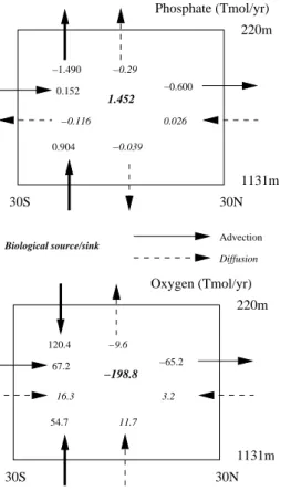
oxygen, phosphorus, radiocarbon, and particle export when compared with data. Fig-ure9 shows the budget of oxygen and phosphorus between 20 S and 20 N and 250– 850 m in this model. Advective fluxes are shown with solid arrows, diffusive fluxes with dashed arrows and biological sources and sinks are in bold italics. Note that the vertical fluxes are not necessarily due to diapycnal processes, isopycnal flows which exchange

20

oxygen-rich and phosphate-poor surface water with oxygen-poor and phosphate-rich intermediate water effectively transport oxygen in the vertical. As can be seen in Fig.9a the upwelling of deep waters acts as an important source of oxygen for the intermediate depths, accounting for approximately 36% of the total oxygen demand. The upwelling also serves as a source of phosphate to the region equivalent to 60% of the phosphate

25

source. This implies that a slowdown in the circulation would reduce mid-depth phos-phate concentrations (and thus presumably the biological cycling of phosphos-phate within

(12)

OSD

EGU

the tropics) by a larger fraction than it would decrease oxygen. Circulation changes brought on by global warming might, therefore, lead to an increase in mid-depth oxy-gen, countering some fraction of the decrease which would be caused by decreased oxygen solubility associated with warming. Further investigation of this, however, will have to await detailed analysis of term budgets in full Earth System Models.

5

In summary, we have shown that global warming changes the balance of waters feeding the intermediate layers, increasing the fraction of younger surface waters and decreasing the fraction of older deep waters. The results of this change are likely to be complex, as the old waters serve as a source of oxygen and nutrients to the subtropical ocean.

10

Acknowledgements. The authors thank the Geophysical Fluid Dynamics Laboratory for support of this research, W. Cooke and R. Slater for their work on including ideal age in the models, and T. Delworth for sharing the results of the R30 run. Comments from K. Rodgers and E. Galbraith are gratefully acknowledged.

References

15

Altabet, M. A., Murray, D. W., and Prell, W. L.: Climatically linked oscillations in Arabian Sea denitrification over the past 1 m.y.: Implications for the marine nitrogen cycle, Paleoceanog-raphy, 14, 732–743, 1999. 806

Delworth, T. L., Stouffer, R. J., Dixon, K. W., Spelman, M. J., Knutson, T. R., Broccoli, A. J., Kushner, P. J., and Wetherald, R. T.: Review of simulations of climate variability and change

20

with the GFDL R30 coupled climate model, Clim. Dyn., 19(7), 555–574, 2002. 808

Delworth, T., Rosati, A., Stouffer, R. J., et al.: GFDL’s global coupled climate models – Part 1: Equilibrium simulations, J. Climate, 18, 643–674, 2006. 808

Elkins, J. W., Wofsy, S. C., McElroy, M. C., Kolb, C. E., and Kaplan, W. E.: Aquatic sources and sinks for nitrous oxide, Nature, 275, 602–606, 1978. 806

25

Galbraith, E. D., Kienast, M., Pedersen, T. F., and Calvert, S. E.: Glacial-interglacial modulation of the marine nitrogen cycle by high-latitude O2 supply to the global thermocline,

(13)

OSD

EGU Gent, P. and McWilliams, J. C.: Isopycnal mixing in ocean circulation models, J. Phys.

Oceanogr., 20, 150–155, 1990. 809

The GFDL Global Atmospheric Model Development Team: The new GFDL global atmosphere and land model AM2-LM2: Evaluation with prescribed SST simulations, J. Climate, 17(24),

4641–4673,2004. 807

5

Gnanadesikan, A., Dunne, J. P., Key, R. M., Matsumoto, K., Sarmiento, J. L., Slater, R. D., and Swathi, P. S.: Oceanic ventilation and biogeochemical cycling: Understanding the phys-ical mechanisms that produce realistic distributions of tracers and productivity, Global

Bio-geochem. Cycles, 18, GB4010, doi:10.1029/2003GB002097, 2004. 814

Gnanadesikan, A., Dixon, K. W., Griffies, S. M., et al.: GFDL’s global coupled climate models –

10

Part 2: The baseline ocean simulation, J. Climate, 18, 675–697, 2006. 808,813

Griffies, S. M., Harrison, M. J., Pacanowski, R. C., and Rosati, A.: A Technical Guide to MOM4. GFDL Ocean Group Technical Report No. 5, Princeton, NJ: NOAA/Geophysical Fluid Dy-namics Laboratory, 2003. 807

Griffies, S. M., Gnanadesikan, A., Dixon, K. W., Dunne, J. P., Gerdes, R., Harrison, M. J.,

15

Rosati, A., Russell, J. L., Samuels, B. L., Spelman, M. J., Winton, M., and Zhang, R: Formu-lation of an ocean model for global climate simuFormu-lations, Ocean Sci., 1, 45–79, 2005. 808 Gruber, N. and Sarmiento, J. L.: Global patterns of marine nitrogen fixation and denitrification,

Global Biogeochem. Cycles, 11, 235–266, 1997. 806

Lin, S.-J.: A “vertically Lagrangian” finite-volume dynamical core for global models, Mon. Wea.

20

Rev., 132(10), 2293–2307, 2004. 807

Luyten, J. L., Pedlosky, J., and Stommel, H. M.: The ventilated thermocline, J. Phys. Oceanogr., 13, 292–309, 1983.

Pacanowski, R., Dixon, K., and Rosati, A.: The GFDL Modular Ocean Model users guide

version 1, GFDL Ocean Group Tech Rep 2, pp. 44, 1991. 809

25

Reid, J. L.: On the total geostrophic circulation of the South Pacific: Flow patterns, tracers and transports, Prog. Oceanogr., 16, 1–61, 1985. 809

Russell, J. L. and Dickson, A. G.: Variability in oxygen and nutrients in South Pacific Antarctic Intermediate Water, Global Biogeochem. Cycles, 17(2), 1033, doi:10.1029/2000GB001317,

2003. 810

30

Russell, J. L., Dixon, K. W., Gnanadesikan, A., Stouffer, R. J., and Toggweiler, J. R.: Southern Ocean Westerlies in a warming world: Propping open the door to the deep ocean, J. Climate, in press, 2006. 811

(14)

OSD

EGU Sarmiento, J. L., Slater, R., Barber, R., Bopp, L., Doney, S. C., Hirst, A. C., Kleypas, J.,

Matear, R., Mikolajewicz, U., Monfray, P., Soldatov, V., Spall, S. A., and Stouffer, R. J.: Re-sponse of ocean ecosystems to global warming, Global Biogeochem. Cycles, 18, GB3003, doi:10.1029/2003GB002134, 2004.

Stouffer, R. J., Weaver, A. J., and Eby, M.: A method for obtaining pre-twentieth century initial

5

conditions for use in climate change studies, Clim. Dyn., 23, 327–339, 2004. 808

Stouffer, R. J., Broccoli, A. J., Delworth, T. L., Dixon, K. W., Gudgel, R., Held, I., Hemler, R., Knutson, T., Lee, H.-C., Schwartzkopf, M. D., Soden, B., Spelman, M. J., Winton, M., and Zeng, F.: GFDL’s CM2 Global Coupled Climate Models – Part 4: Idealized Climate Response, J. Climate, 19, 723–740, 2006. 808,813

10

Vecchi, G. A., Soden, B. J., Wittenberg, A. T., Held, I. M., Leetmaa, A., and Harrison, M. J.: Weakening of tropical Pacific atmospheric circulation due to anthropogenic forcing, Nature,

441(7089), 73–76, 2006. 807

Wallmann, K.: Feedbacks between oceanic redox states and marine productivity: A model perspective focused on benthic phosphorus cycling, Global Biogeochem. Cycles, 17, 1084,

15

(15)

OSD

EGU

Fig. 1. Oxygen minimum zones, age and potential vorticity in models and data at 300 m in

the Central Pacific. (a) Oxygen (colors) and CFC-12 age (contours). The edge of the oxygen

minimum zone occurs in a region of strong age gradients. Note also the asymmetry between the Northern and Southern zones. (b) Potential vorticity (colors) and CFC age (contours) for

same region. The boundary of the old waters corresponds to a boundary between stratified interior waters (high PV) and weakly stratified waters in the shadow zone (low PV).(c) Potential

vorticity (colors) and ideal age (contours) in model CM2.0, 67.5 years after the start of the 1990 control run. While ideal age is not directly comparable to CFC age, many of the same features are seen in the model as in the data.(d) Potential vorticity and ideal age in CM2.1 model 67.5

(16)

OSD

EGU

Fig. 2. Age changes under global warming (second century of 2×CO2 – 1860 control). Note

that scale is linear from −60 to 60 years, with extreme age changes being shown by the most extreme colors. (a) CM2.0 at 300 m. (b) CM2.0 at 800 m. (c) CM2.1 at 300 m (d) CM2.1 at

(17)

OSD

EGU

Fig. 3. Average changes in age under global warming. (a) CM2.0 (b) CM2.1 (c) R30 model (d)

(18)

OSD

EGU

Fig. 4. Volume of “young” water (with an ideal age less than 50 years) in the CM2 series. Solid

(19)

OSD

EGU

Fig. 5. Time series of the ideal age at 300 m in the CM2 series. Black lines are for CM2.0, red

for CM2.1. Lines with symbols are the doubled CO₂run. (A) Eastern Tropical North Pacific.

Note that the ages under global warming begin to diverge about year 50. (B) Subpolar North

Pacific. Note substantial decacal variability of same order of magnitude as climate change.(C)

Peru Current. Here the difference between the ages cannot be attributed to spinup alone, as year 80 of the control CM2.1 is still substantially younger than CM2.0. (D) Southern Ocean.

The same difference in age is attributable to a difference in ventilation forced by the higher Southern Ocean winds.

(20)

OSD

Printer-friendly Version Interactive Discussion EGU 0 500 1000 1500 2000 2500 −4000 −3000 −2000 −1000 0

1D model of Ideal Age, K

v=0.1 Solid: Mu=36 Sv Dashed: Mu=18 Sv

(a)

Age in Years Depth in m 0 500 1000 −4000 −3000 −2000 −1000 0

1D model of Ideal Age, K

v=1 Solid: Mu=36 Sv Dashed: Mu=18 Sv

(b)

Age in Years Depth in m 0 500 1000 1500 2000 −4000 −3000 −2000 −1000 0

Age Change (Reduced Upwelling) K

v=0.1

(c)

Age in Years Depth in m −50 0 50 100 150 −4000 −3000 −2000 −1000 0

Age Change (Reduced Upwelling) K

v=1

(d)

Age in Years

Depth in m

Fig. 6. Solutions generated by a one-dimensional advective-diffusive model of ideal age. In

left-hand column, solutions are shown for wD/Kv=40, 20 (w=0.5,1×10

−7

m/s corresponding to 18 and 36 Sv of upwelling and Kv=10

−5

m2/s=0.1 cm2/s). In right hand column solutions are shown for lower values of wD/Kv(4,2) corresponding to the same pair of upwelling values and

a higher diffusive of 1 cm2

(21)

OSD

EGU

Fig. 7. Budget of age in CM2.1 models. Age budget is scaled relative to the volume of the

ocean, so that a flux of 1 would mean that the flux was accounting for all of the aging in the ocean below the surface layer. (a) Advective age flux, showing a significant decrease in

the advective flux under global warming. (b) Diffusive age flux (convection+implicit vertical

diffusion+isopycnal mixing and advection) showing a relatively small change in this flux. (c) Flux changes under global warming. Decrease in advective flux dominates, accounting for decrease in age above 2000 m and increase in age below that point.

(22)

OSD

EGU

Fig. 8. Overturning change under global warming associated with the three models. Contour

(23)

OSD

Printer-friendly Version Interactive Discussion EGU 0.904 1.452 −0.039 0.152 0.026 −0.116 Phosphate (Tmol/yr) 220m 1131m 30S 30N −0.600 −0.29 −1.490 Advection Diffusion Biological source/sink 220m 1131m 30S 30N Oxygen (Tmol/yr) −198.8 120.4 −9.6 54.7 11.7 3.2 67.2 16.3 −65.2

Fig. 9. Budgets of phosphate (left) and oxygen (right) in the 220–1131 m depth range from

30 S to 30 N in the PRINCE2A model of Gnanadesikan et al. (2004). Solid lines are advective fluxes, dashed lines mixing fluxes. The italicized bold numbers indicate biological sources or sinks. Upwelling from below 1100 m supplies a significant amount of phosphate and oxygen to this region.