ANALYTICS OF SEQUENTIAL TIME DATA FROM PHYSICAL ASSETS
AHMED ELSHEIKH
DÉPARTEMENT DE MATHÉMATIQUES ET DE GÉNIE INDUSTRIEL ÉCOLE POLYTECHNIQUE DE MONTRÉAL
THÈSE PRÉSENTÉE EN VUE DE L’OBTENTION DU DIPLÔME DE PHILOSOPHIAE DOCTOR
(GÉNIE INDUSTRIEL) AVRIL 2018
ÉCOLE POLYTECHNIQUE DE MONTRÉAL
Cette thèse intitulée :
ANALYTICS OF SEQUENTIAL TIME DATA FROM PHYSICAL ASSETS
présentée par : ELSHEIKH Ahmed
en vue de l’obtention du diplôme de : Philosophiae Doctor a été dûment acceptée par le jury d’examen constitué de :
M. ADJENGUE Luc Désiré, Ph. D., président
Mme YACOUT Soumaya, D. Sc., membre et directeur de recherche
M. OUALI Mohamed-Salah, Doctorat, membre et codirecteur de recherche M. BASSETTO Samuel Jean, Doctorat, membre
RÉSUMÉ
Avec l’avancement dans les technologies des capteurs et de l’intelligence artificielle, l'analyse des données est devenue une source d’information et de connaissance qui appuie la prise de décisions dans l’industrie. La prise de ces décisions, en se basant seulement sur l’expertise humaine n’est devenu suffisant ou souhaitable, et parfois même infaisable pour de nouvelles industries. L'analyse des données collectées à partir des actifs physiques vient renforcer la prise de décisions par des connaissances pratiques qui s’appuient sur des données réelles. Ces données sont utilisées pour accomplir deux tâches principales; le diagnostic et le pronostic.
Les deux tâches posent un défi, principalement à cause de la provenance des données et de leur adéquation avec l’exploitation, et aussi à cause de la difficulté à choisir le type d'analyse. Ce dernier exige un analyste ayant une expertise dans les déférentes techniques d’analyse de données, et aussi dans le domaine de l’application. Les problèmes de données sont dus aux nombreuses sources inconnues de variations interagissant avec les données collectées, qui peuvent parfois être dus à des erreurs humaines. Le choix du type de modélisation est un autre défi puisque chaque modèle a ses propres hypothèses, paramètres et limitations.
Cette thèse propose quatre nouveaux types d'analyse de séries chronologiques dont deux sont supervisés et les deux autres sont non supervisés. Ces techniques d'analyse sont testées et appliquées sur des différents problèmes industriels. Ces techniques visent à minimiser la charge de choix imposée à l'analyste.
Pour l’analyse de séries chronologiques par des techniques supervisées, la prédiction de temps de défaillance d’un actif physique est faite par une technique qui porte le nom de ‘Logical Analysis of Survival Curves (LASC)’. Cette technique est utilisée pour stratifier de manière adaptative les courbes de survie tout au long d’un processus d’inspection.
Ceci permet une modélisation plus précise au lieu d'utiliser un seul modèle augmenté pour toutes les données. L'autre technique supervisée de pronostic est un nouveau réseau de neurones de type ‘Long Short-Term Memory (LSTM) bidirectionnel’ appelé ‘Bidirectional Handshaking LSTM (BHLSTM)’. Ce modèle fait un meilleur usage des séquences courtes en faisant un tour de ronde à travers les données. De plus, le réseau est formé à l'aide d'une nouvelle fonction objective axée sur la sécurité qui force le réseau à faire des prévisions plus sûres. Enfin, étant donné que LSTM est une technique supervisée, une nouvelle approche pour générer la durée de vie utile restante
(RUL) est proposée. Cette technique exige la formulation des hypothèses moins importantes par rapport aux approches précédentes.
À des fins de diagnostic non supervisé, une nouvelle technique de classification interprétable est proposée. Cette technique est intitulée ‘Interpretable Clustering for Rule Extraction and Anomaly Detection (IC-READ)’. L'interprétation signifie que les groupes résultants sont formulés en utilisant une logique conditionnelle simple. Cela est pratique lors de la fourniture des résultats à des non-spécialistes. Il facilite toute mise en œuvre du matériel si nécessaire. La technique proposée est également non paramétrique, ce qui signifie qu'aucun réglage n'est requis. Cette technique pourrait également être utiliser dans un contexte de ‘one class classification’ pour construire un détecteur d'anomalie. L'autre technique non supervisée proposée est une approche de regroupement de séries chronologiques à plusieurs variables de longueur variable à l'aide d'une distance de type ‘Dynamic Time Warping (DTW)’ modifiée. Le DTW modifié donne des correspondances plus élevées pour les séries temporelles qui ont des tendances et des grandeurs similaires plutôt que de se concentrer uniquement sur l'une ou l'autre de ces propriétés. Cette technique est également non paramétrique et utilise la classification hiérarchique pour regrouper les séries chronologiques de manière non supervisée. Cela est particulièrement utile pour décider de la planification de la maintenance. Il est également montré qu'il peut être utilisé avec ‘Kernel Principal Components Analysis (KPCA)’ pour visualiser des séquences de longueurs variables dans des diagrammes bidimensionnels.
ABSTRACT
Data analysis has become a necessity for industry. Working with inherited expertise only has become insufficient, expensive, not easily transferable, and mostly unavailable for new industries and facilities. Data analysis can provide decision-makers with more insight on how to manage their production, maintenance and personnel. Data collection requires acquisition and storage of observatory information about the state of the different production assets. Data collection usually takes place in a timely manner which result in time-series of observations.
Depending on the type of data records available, the type of possible analyses will differ. Data labeled with previous human experience in terms of identifiable faults or fatigues can be used to build models to perform the expert’s task in the future by means of supervised learning. Otherwise, if no human labeling is available then data analysis can provide insights about similar observations or visualize these similarities through unsupervised learning. Both are challenging types of analyses.
The challenges are two-fold; the first originates from the data and its adequacy, and the other is selecting the type of analysis which is a decision made by the analyst. Data challenges are due to the substantial number of unknown sources of variations inherited in the collected data, which may sometimes include human errors. Deciding upon the type of modelling is another issue as each model has its own assumptions, parameters to tune, and limitations.
This thesis proposes four new types of time-series analysis, two of which are supervised requiring data labelling by certain events such as failure when, and the other two are unsupervised that require no such labelling. These analysis techniques are tested and applied on various industrial applications, namely road maintenance, bearing outer race failure detection, cutting tool failure prediction, and turbo engine failure prediction. These techniques target minimizing the burden of choice laid on the analyst working with industrial data by providing reliable analysis tools that require fewer choices to be made by the analyst. This in turn allows different industries to easily make use of their data without requiring much expertise.
For prognostic purposes a proposed modification to the binary Logical Analysis of Data (LAD) classifier is used to adaptively stratify survival curves into long survivors and short life sets. This model requires no parameters to choose and completely relies on empirical estimations. The proposed Logical Analysis of Survival Curves show a 27% improvement in prediction accuracy
than the results obtained by well-known machine learning techniques in terms of the mean absolute error.
The other prognostic model is a new bidirectional Long Short-Term Memory (LSTM) neural network termed the Bidirectional Handshaking LSTM (BHLSTM). This model makes better use of short sequences by making a round pass through the given data. Moreover, the network is trained using a new safety oriented objective function which forces the network to make safer predictions. Finally, since LSTM is a supervised technique, a novel approach for generating the target Remaining Useful Life (RUL) is proposed requiring lesser assumptions to be made compared to previous approaches. This proposed network architecture shows an average of 18.75% decrease in the mean absolute error of predictions on the NASA turbo engine dataset.
For unsupervised diagnostic purposes a new technique for providing interpretable clustering is proposed named Interpretable Clustering for Rule Extraction and Anomaly Detection (IC-READ). Interpretation means that the resulting clusters are formulated using simple conditional logic. This is very important when providing the results to non-specialists especially those in management and ease any hardware implementation if required. The proposed technique is also non-parametric, which means there is no tuning required and shows an average of 20% improvement in cluster purity over other clustering techniques applied on 11 benchmark datasets. This technique also can use the resulting clusters to build an anomaly detector.
The last proposed technique is a whole multivariate variable length time-series clustering approach using a modified Dynamic Time Warping (DTW) distance. The modified DTW gives higher matches for time-series that have the similar trends and magnitudes rather than just focusing on either property alone. This technique is also non-parametric and uses hierarchal clustering to group time-series in an unsupervised fashion. This can be specifically useful for management to decide maintenance scheduling. It is shown also that it can be used along with Kernel Principal Components Analysis (KPCA) for visualizing variable length sequences in two-dimensional plots. The unsupervised techniques can help, in some cases where there is a lot of variation within certain classes, to ease the supervised learning task by breaking it into smaller problems having the same nature.
TABLE OF CONTENTS
RÉSUMÉ ... iii
Abstract ... v
Table of Contents ... vii
List of Tables ... xi
List of Figures ... xiii
List of Abbreviations ... xv
Chapter 1 Introduction ... 1
1.1 Data in Industry ... 2
1.1.1 Variation in Time-Series Lengths ... 4
1.1.2 Types of Time-Series Data Available in Industry ... 4
1.1.3 Types of Analysis Tasks in Industry ... 5
1.1.4 Potentials for Data Analysis in Industry ... 6
1.1.5 Anticipated Gains from Data Analysis ... 6
1.2 Problem Statement ... 7 1.3 General Objective ... 8 1.4 Specific Objectives ... 8 1.5 Originality of Research ... 9 1.6 Thesis Organization ... 10 1.7 Deliverables ... 11
Chapter 2 Critical Literature Review ... 14
2.1 Statistical Modelling ... 15
2.2 Discriminative Modelling ... 16
2.3 Instance-Based Learning ... 18
2.4 Rule Induction ... 19
Chapter 3 Article 1: Failure Time Prediction Using Logical Analysis of Survival Curves and Multiple Machining Signals of a Nonstationary Process ... 20
3.1 Literature review ... 20
3.2 Methodology ... 22
3.2.1 Logical Analysis of Data (LAD) ... 23
3.2.2 Kaplan-Meier Survival Curve ... 23
3.2.3 Logical Analysis of Survival Curves (LASC)... 24
3.3 Experimental Application ... 28 3.3.1 Data Acquisition ... 28 3.3.2 Data Preprocessing ... 28 3.3.3 Data Analysis ... 29 3.4 Results ... 31 3.5 Discussion ... 33
3.6 Using LASC for Decision Making ... 36
3.7 Conclusion ... 38
Chapter 4 Article 2: Bidirectional Handshaking LSTM for Remaining Useful Life Prediction ………40
4.1 Introduction ... 40
4.2 The Long Short-Term Memory Cell ... 44
4.2.1 Bidirectional LSTM ... 45
4.3 The Proposed Methodology ... 45
4.3.2 Safety-Oriented Objective Function ... 46
4.3.3 Target RUL Generation ... 47
4.3.4 Data Preparation ... 50
4.4 Experiments and Results ... 50
4.4.1 Benchmark Dataset Overview ... 50
4.4.2 Performance Measures ... 51
4.4.3 Performance Evaluation Using Different Network Architectures ... 51
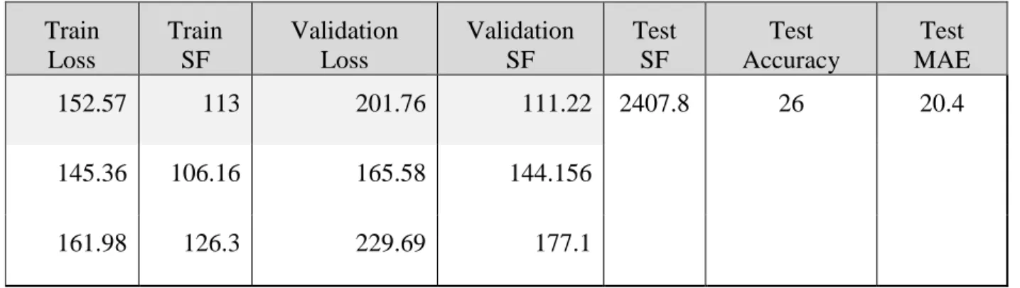
4.4.4 Performance Evaluation Using the Mean Squared Error with BHSLTM ... 54
4.4.5 Performance Evaluation Using the Piecewise Linear Target RUL ... 56
4.5 Discussion and Conclusion ... 56
Chapter 5 Article 3: A Profile Favoring Dynamic Time Warping for the Hierarchical Clustering of Systems Based on Degradation ... 58
5.1 Introduction ... 58
5.2 Time-series Clustering ... 61
5.3 Dynamic Time Warping (DTW) ... 63
5.3.1 Finding the minimum Warping Path ... 64
5.3.2 Profile Favoring DTW ... 65
5.4 Hierarchal Clustering ... 67
5.4.1 Procedure for Bottom-Up Hierarchal Clustering ... 67
5.4.2 Effect of Profile Favoring DTW on Clustering ... 68
5.5 Example of an application ... 70
5.5.1 Cluster Validity Indices ... 72
5.5.2 Results Using a Single Road-Performance Metric ... 73
5.5.3 Results Using Multiple Road-Performance Metrics ... 74
Chapter 6 Article 4: Interpretable Clustering for Rule Extraction and Anomaly Detection:
A New Unsupervised Rule Induction Technique ... 79
6.1 Introduction ... 79
6.2 Interpretable Clustering for Rule Extraction and Anomaly Detection (IC-READ) ... 84
6.2.1 Identifying Split Candidates ... 84
6.2.2 Selecting the Best Split ... 87
6.2.3 Rule Set Identification ... 89
6.3 Benchmark Dataset Examples ... 90
6.3.1 Experimental Setup ... 90
6.4 IC-READ Beyond Clustering ... 94
6.5 IC-READ for Anomaly Detection ... 95
6.6 Experimental Setup ... 96
6.7 Results ... 97
6.8 Conclusion ... 99
6.9 Appendix ... 101
6.9.1 Pseudo Code for Main Program ... 101
6.9.2 Pseudo Code for 𝑮𝒆𝒕𝑪𝒂𝒏𝒅𝒊𝒅𝒂𝒕𝒆𝑪𝒖𝒕𝒑𝒐𝒊𝒏𝒕𝒔(𝑿) ... 101
6.9.3 Pseudo Code for 𝑮𝒆𝒕𝑪𝒂𝒏𝒅𝒊𝒅𝒂𝒕𝒆𝑳𝒂𝒃𝒆𝒍𝒔(𝑪𝑷, 𝑩) ... 102
6.9.4 Pseudo Code for 𝑬𝒗𝒂𝒍𝒖𝒂𝒕𝒆𝑬𝒂𝒄𝒉𝑪𝒂𝒏𝒅𝒊𝒅𝒂𝒕𝒆(𝑳𝑩, 𝑿) ... 102
6.9.5 Pseudo Code for 𝑲𝒆𝒆𝒑𝑵𝑩𝒆𝒔𝒕𝑪𝒂𝒏𝒅𝒊𝒅𝒂𝒕𝒆𝒔(𝑬𝑽, 𝑪𝑷, 𝑳𝑩) ... 103
Chapter 7 General Discussion ... 104
Chapter 8 Conclusions and Recommendations ... 107
8.1 Future Work ... 112
LIST OF TABLES
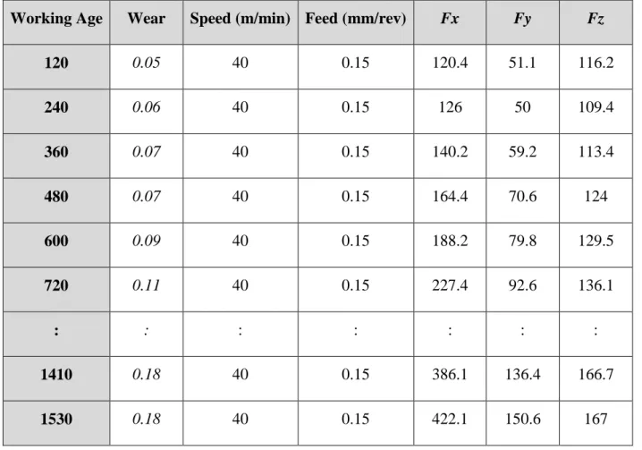
Table 3.1 Force readings and corresponding wear event for the illustrative example ... 26
Table 3.2 Patterns extracted at 𝑡12 in the illustrative example ... 26
Table 3.3 A snippet of the data collected in the lab experiments ... 29
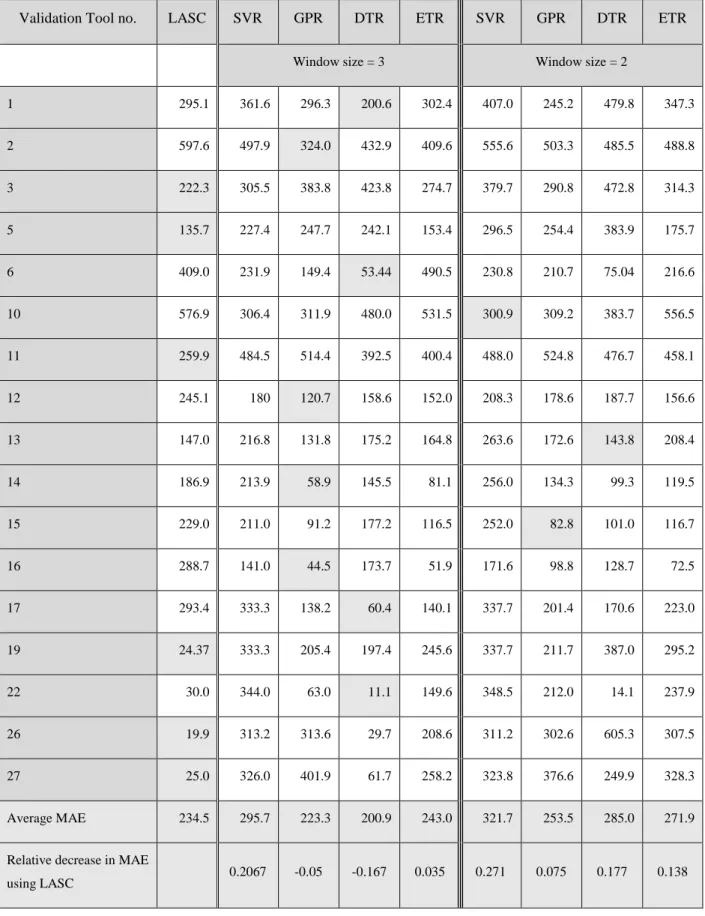
Table 3.4 MAE using leave-one-out cross-validation for different RUL predictors. ... 34
Table 3.5 Summary of Potentials and Limitations of LASC ... 39
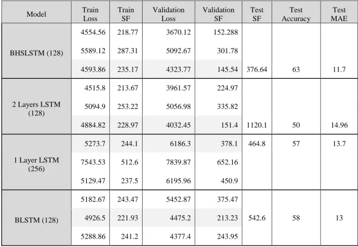
Table 4.1 Dataset 1 performance measures for different network architectures. ... 53
Table 4.2 Dataset 3 performance measures for different network architectures. ... 53
Table 4.3 Bidirectional LSTM performance without the proposed handshake procedure for dataset 1. ... 54
Table 4.4 BHLSTM performance using the MSE objective function for dataset 1. ... 54
Table 4.5 BHLSTM performance using the MSE objective function for dataset 3. ... 54
Table 4.6 BHLSTM performance on dataset 1 using the piecewise linear RUL. ... 56
Table 4.7 Summary of Potentials and Limitations of BHLSTM ... 57
Table 5.1 Comparison of DTW distances for the UTS synthetic example. ... 66
Table 5.2 Single-metric road-degradation data cluster validity summary of results. ... 75
Table 5.3 MTS data cluster validity summary of results. ... 76
Table 5.4 Summary of Potentials and Limitations of PFDTW ... 78
Table 6.1 Benchmark UCI datasets' discribtion. ... 90
Table 6.2 Performance comparison between different clustering techniques on benchmark UCI datasets. ... 93
Table 6.3 Comparison of the induced rules by the IC-READ-CH and the supervised decision trees. ... 94
Table 6.4 Shuttle dataset performance comparison for different anomalous fraction values. ... 98
Table 6.6 Ranges of normal operation on each feature identified by the IC-READ-CH anomaly detection procedure. ... 99 Table 6.7 Summary of Potentials and Limitations of IC-READ ... 103 Table 8.1 Summary of proposed techniques and achievements of the thesis objectives ... 109
LIST OF FIGURES
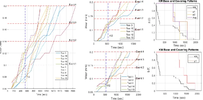
Figure 3.1 Example of analysis at time sample t12 and split using event 1; (mid-top) Tools having wear at time t12 above event 1; (mid-bottom) Tools having wear at time t12 below event 1; (top-right) KM curves constructed from the failure time of the tools covered by patterns 𝑝1, 𝑝2, and their average calculated using equation 4; (bottom-right) KM curve constructed
from the tools covered by pattern 𝑝1. ... 25
Figure 3.2 Tool wear vs. time showing wear states and analysis times, with linear interpolation between measurements. The variation in failure times is due to different operating conditions. ... 30
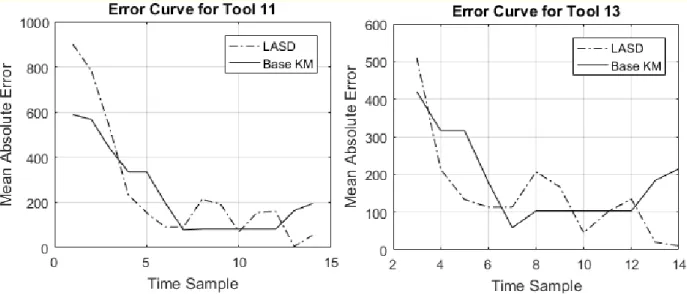
Figure 3.3 LASC and KM MAE performance vs time for tools of the classified tools ... 36
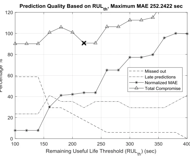
Figure 3.4 Compromise between the three decision quality factors to find the reliable decision based upon the choice of the RULth ... 38
Figure 4.1 LSTM cell diagram ... 45
Figure 4.2 BHLSTM diagram for a single forward and a single backward LSTM cells ... 46
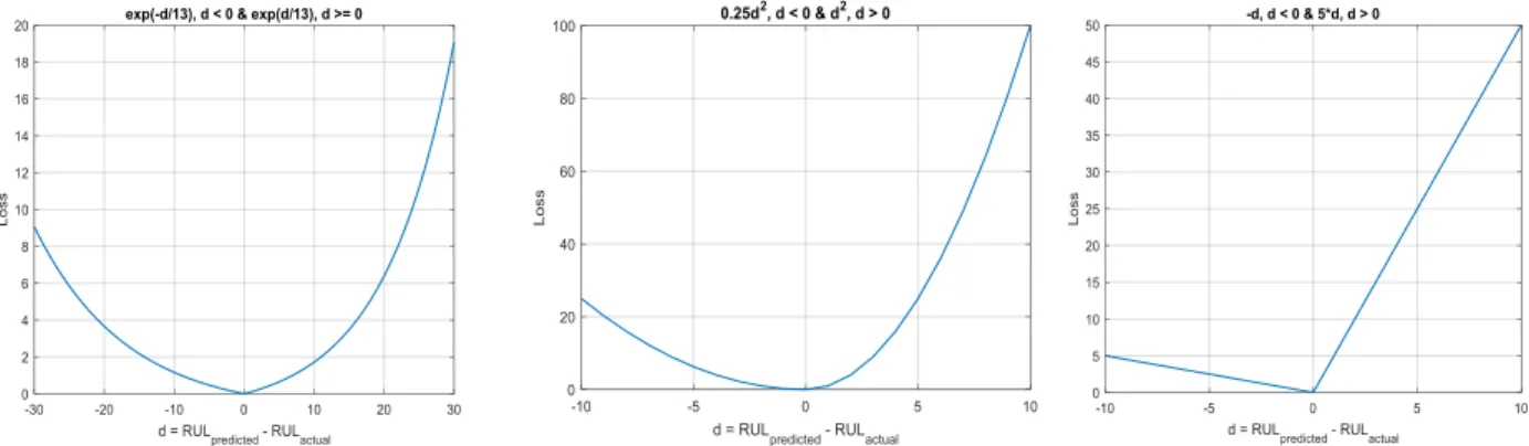
Figure 4.3 Comparison between the scoring function 𝛼1 = 10, 𝛼2 = 13 (left), the proposed asymmetric squared objective function 𝛼1 = 0.25, 𝛼2 = 1 (middle), and the asymmetric absolute objective function 𝛼1 = 1, 𝛼2 = 5 (right). ... 48
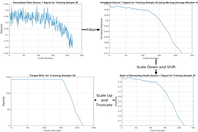
Figure 4.4 RUL target generation procedure. ... 49
Figure 4.5 Comparison between RUL forecasts using ASE and MSE objective functions. ... 55
Figure 5.1 Warping path between two univariate time-series. ... 65
Figure 5.2 Illustrative example for comparing DTW distances for UTS. ... 66
Figure 5.3 Example UTS with different modes of behavior. ... 68
Figure 5.4 Visual Comparison between the variants if the DTW distances in the low dimensional KPCA projection. ... 69
Figure 5.5 Comparison between the dendograms of the DTW distances. ... 70
Figure 5.6 Metric of real data on the degradation of road segments versus observation sequence. ... 71
Figure 5.7 DTW clustering results. ... 75 Figure 5.8 DTW with alignment clustering results. ... 75 Figure 5.9 Profile favoring DTW clustering results. ... 76 Figure 6.1 (Top) The raw observation space and marginal histograms, (Middle) clustering using
candidate splits from the original raw observation space, and (Bottom) clusters using the adaptive splitting procedure. ... 86 Figure 6.2 Modes of operation within a single class. ... 95 Figure 6.3 Example of 2D anomaly detection using IC-READ-CH using hyper-rectangle tightening
with anomalous fraction 0.1. ... 96 Figure 6.4 Widowing procedure used for feature extraction. ... 97 Figure 8.1 Summary of the proposed techniques ... 107
LIST OF ABBREVIATIONS
AAE Asymmetric Absolute ErrorANN Artificial Neural Networks ARI Adjusted Rand Index
ARIMA Autoregressive Integrated Moving Average ARMA Autoregressive Moving Average
ASE Asymmetric Squared Error
BHLSTM Bidirectional Handshaking LSTM CBM Condition Based Maintenance
CH Calinski–Harabasz
CMAPSS Commercial Modular Aero-Propulsion System Simulation DB* Modified Davies–Bouldin
DDTW Differential Dynamic Time Warping DFT Discrete Fourier transform
DNF Disjunctive Normal Form DTR Decision Tree Regression DTW Dynamic Time Warping DWT Discrete Wavelet Transform ED Euclidean Distance
EM Expectation-Maximization ETR Ensemble Tree Regression
FCM Fuzzy C-Means
FFNN Feed Forward Neural Network GMM Gaussian Mixture Model GPR Gaussian Process Regression HC Hierarchal clustering
HMM Hidden Markov Model
IC-READ Interpretable Clustering for Rule Extraction and Anomaly Detection IRI International Roughness Index
KM Kaplan-Meier
KM K-Means
KPCA Kernel Principal Components Analysis LAD Logical Analysis of Data
LASC Logical Analysis of Survival Cuves LSTM Long Short-Term Memory
MAE Mean Absolute Error MSE Mean Squared Error
MTMDET Ministère des Transports de la Mobilité Durable et de l’Électrification des Transports
MTS Multivariate Time-Series
NN Neural Network
OCC One-Class Classification
OCCSVM One-Class Classification Support Vector Machine PCA Principal Components Analysis
PDDP Principal Direction Divisive Partitioning PM Predictive Maintenance
PSD Power Spectral Density RNN Recurrent Neural Network RUL Remaining Useful Life
SF Scoring Function
Sil Silhouette Index
SVM Support Vector Machine SVR Support Vector Regression
TQ Transport Quebec
VLMTS Variable Length Multivariate Time-Series VLUTS Variable Length Univariate Time-series
CHAPTER 1
INTRODUCTION
Since the beginning of the industrial revolution in the seventieth century, various physical assets came to existence and have been growing in number ever since. Maintenance evolved over the history of industry starting from replacement on failure, to scheduled maintenance, Condition Based Maintenance (CBM) (Vogl, Weiss, and Helu 2016), and finally to Predictive Maintenance (PM). Every physical asset, no matter how good its crafting quality is, undergoes degradation. The difference is rate of degradation (Jardine, Lin, and Banjevic 2006). This means that intervention for maintenance or replacement is inevitable. As the industry scale grew as well as the number and variety of physical assets increased, the need for wise management increased (Canfield 1986). Furthermore, compromising asset replacement, maintenance, and downtime cost with profit has become a critical issue (Venkatasubramanian 2005).
CBM is currently the most abundant working maintenance system due to its relative simplicity as it only requires few sensors, reduced cost as it does not require intensive data collection, and it shows noticeable improvements in reducing production costs and increasing uptime (Ahmad and Kamaruddin 2012). On the other hand, PM aims not only at detection of near failures but also at predicting the future behavior given current working conditions. Having an insight about the asset’s behavior allows more efficient management and production (Lee, Ghaffari, and Elmeligy 2011; Saxena et al. 2010).
PM faces a multitude of challenges that needs to be overcome in order to obtain reliable performance (Vogl, Weiss, and Helu 2016). Firstly, data acquisition is not yet optimal in most scenarios (Hess, Calvello, and Frith 2005). This is because most transducers are affected by their surrounding environment which is inherited from their semi-conductor nature. In turn, clever processing proceeded by smart decision making is a must to overcome the inherited electronic sensor problems.
Secondly, the system complexity and interaction between its various subsystems may not be well represented by a simple model (Hess, Calvello, and Frith 2005). Also, some systems exhibit multiple modes of operation which are not controlled or intentional due to the working environment. Examples of such assets are city roads with different usage rates and weather conditions (Ben-Akiva and Ramaswamy 1993), and aircraft engines (Korson et al. 2003). These assets undergo change and sometimes end up in unknown, or unexpected operating conditions.
Uncovering groups of behavior and finding structure in the gathered data can be beneficial for decision making as well as making design precautions, and maintenance planning.
Experience is gained throughout time. Hence, to make better decisions regarding the future, one must make use of the previous experiences. Therefore, the regard for time adaptive prognostics can result in better management decisions. The growing data availability from different industrial plants, and the advancements in its acquisition techniques opens up a myriad of opportunities (Abellan-Nebot and Subrión 2009). Discovering a hidden structure in newly observed raw data can be very beneficial to proactive decision making (Jardine et al. 2015; Vogl, Weiss, and Helu 2016). Data concern all available observations that characterize the system state condition and its behavior over time. For some applications such as machine diagnosis (Mohamad-ali, Yacout, and Lakis 2014), or product quality inspections (Tiejian Chen et al. 2016), the data collected at different time intervals can be treated as independent. However, when the sequence of observations is highly correlated (Ghasemi, Yacout, and Ouali 2010) as normally expected from degradation and maintenance processes, these observations have to be considered as time-series.
There are two main types of information that can be extracted by time-series analysis of physical-asset data; diagnostic and prognostic. Diagnosis is mainly concerned about monitoring the current state of the working physical asset giving indication of its current health state or operation state. On the other hand, prognosis is oriented towards prediction of future states of the working asset. Predictions are more insightful and hence can help achieve more efficient production (Guillén et al. 2016).
For both diagnosis and prognosis, dealing with time-series instead of instantaneous readings independently means that the relation between observations through time should be modelled and not just the mapping between the observations and the targeted diagnostic or prognostic objective. This modelling can be either explicit in the used model or implied by how the time-series is inputted to the model.
1.1 Data in Industry
Data collected by industrial firms are mainly collected in a timely manner. The data collected is some sort of observable aspect that can be either:
2- Related to the load exerted on the asset such as torque.
Data can be collected in a fully automatic, semi-automatic, or manual as follows:
1- Fully automatic data collection means that the sensor is placed on the assets such as a vibration sensor or near it such as an acoustic emission sensor and the sensor readings are continuously stored in some database.
2- Semi-automatic data collection means that the sensor needs to be moved to the asset to make the desire data collection. This is the case when the desired useful aspects of the asset require placement of a large number of expensive sensors such as laser sensors used for road inspection. Of course, it is not practical to place such sensors on all roads, instead the sensor is vehicle mounted and moves to each location.
3- Manual data collection requires a human expert to go and inspect the asset and estimate certain aspects for the asset based on observation or according to a certain inspection code. Another type of manual recording is the recording of human intervention to do maintenance for example.
Collection of data is vulnerable to errors due to various reasons such as:
Interaction between different assets with each other makes the sensor gather the effect of interaction and not purely the readings for the observed asset.
Interaction between the assets and sensors with the environment. Electronic sensors change their characteristics with temperature for example.
Intervention of a human factor in the data collection procedure. Even in the case of fully automated data collection, a human expert sometimes intervenes to identify the observations that experience a certain damage, fault, or state of operation. The human factor is the highest source of errors in data collection. Human errors can be in the form of missing data, wrong identification, or misuse of the portable sensor, which in turn can be hard to recover or even sometimes misleading.
Handling several types of errors is considered as a pre-processing step to clean the data and restore as much as possible from the originally intended data for the subsequent analysis step. Another intermediate step prior to analysis is called feature extraction, which aims at feeding the analysis
step with lesser varying information such as extracting the frequencies evident in a vibration signal instead of giving the analysis step the raw sensor recordings at each instant.
Analyzing data means either extracting useful information from the data or fulfilling a certain task such as classifying modes of operation based on historically labeled data. Data analysis can either be done offline, which means after data collection has ended the analysis uses these records to build a model, or online, which means that the analysis model is updated concurrently with the data collection.
When data analysis is given a specific task to learn then it is called supervised learning. On the other hand, if no specific task is required then it is called unsupervised learning and aims at finding interesting relations between different training records.
1.1.1 Variation in Time-Series Lengths
Recorded data usually have variable lengths, like for example when the inspected assets have variable run-to-failure spans. This variation in the length of the collected sequences of observations is handled by one of the following four ways:
1) Truncation, which means trimming all of the data to match the shortest sequence.
2) Padding, which means adding filler values to the data, like zeros for example, to match the maximum length sequence of data.
3) Windowing, which means analyzing shorter sub-sequences from the original sequence, such that these windows of observation have equal lengths.
4) Using techniques that can perform analysis on variable length sequences.
The first and second ways of handling are not suitable for sequences of large variation since the information they contain are either lost by truncation or distorted by too much padding. Nevertheless, the online type of analysis is obliged to use the windowing approach since the outcomes of the analysis are required concurrently with the monitoring process.
1.1.2 Types of Time-Series Data Available in Industry
There are several types of time-series data that can be available from industry. Here the main types of data that are encountered in industry:
1- Run-to-failure data: this type of data contains a sequence of observations that were collected as the assets started working in the system at full health, until it failed. The identification and definition of failure can be different from one system to another, even for the same asset. The identification then requires an external observer to label or annotate at a certain time the type of failure for the asset. This external observer might be a human or another device such as a computer vision camera.
2- Truncated data: this type of data is the same as the above, but there is no clear indication at what initial state the asset was when the data collection started. This is the most practical case because the asset can enter the system in a used state, undergo partial maintenance, or the manufacturing of the asset itself is not perfect, which is usually the case.
3- Data collected without annotation: this type of data has no labelling of events given from an external observer to identify certain types of failure or fatigue to the asset during its monitoring.
4- Non-event data: this type of data is either collected from critical assets that undergo extensive preventive maintenance, such as nuclear reactors, or from new assets that were not used before, such as a new power generator. Data available from this scenario usually belongs to one mode of operation, which is normal operation. This sort of data can be useful for anomaly detection, which is out of the norm behavior.
1.1.3 Types of Analysis Tasks in Industry
Supervised Learning Analysis
Supervised analysis in industry is either diagnostic or prognostic. Diagnosis is concerned with identifying the current state of the asset while prognosis tries to predict the future state(s) of the asset. Both tasks require the historical data observations to be labeled with the states or conditions that will be estimated by the analysis. In other words, supervised data analysis tries to identify relationships between the observations and the labels to perform the task on its own to decrease the reliance on human expertise.
Moreover, automated diagnosis and prognosis provide industrial systems with an around the clock inspection for any number of assets without the need of a huge number of expert technicians working in shifts.
Unsupervised Learning Analysis
This type of analysis is specifically useful for either new industries, or old industries trying to make use of historical data. Since for both cases labelling was not taken into consideration while collecting the data or there are no experts for this new type of data, both end up with just records of observations. In this case there are two types analyses to be conducted:
1- Clustering: which means grouping different records of data that show similar behavior or similar readings. Of course, similar in this context does not mean exactly the same, but rather a like.
2- Anomaly/Novelty detection: This means that it is known that the recorded data belonged only to one condition, which is typically the normal operating condition. Hence, the unsupervised data analysis task in this case is to identify if asset is in a state that is out of the norm which was seen before.
1.1.4 Potentials for Data Analysis in Industry
Industrial capital is mainly divided into materials, physical assets and personnel. Each of these components contribute to the total expenditure with a varying proportion depending on the type of industry. Data analysis can provide the decision makers with insights on how to benefit the most from each component in their industrial firm. Faults and failures can result in a lot of wasted material, costly maintenance, and prolonged downtime losses (Venkatasubramanian 2005; Vogl, Weiss, and Helu 2016). Making accurate in-time predictions allows the industry to benefit the most from their assets without neither making early unnecessary maintenance nor late replacement maintenance. The value analysis of maintenance show an exponential increase when proper intervention takes place (Haddad, Sandborn, and Pecht 2012).
A study on the impact of maintenance on competitiveness and profitability of weaving industry show that an improvement in production quality comes as a by product from better maintenance, as well as a reduction in the number of required spare parts (Maletič et al. 2014).
1.1.5 Anticipated Gains from Data Analysis
There are yet very few studies that measure the benefits of applying data analysis to industrial profit although it has been already applied in many industries.
This is due to the variability in the different types of industries and their decision-making procedures.
Nevertheless, for electronic asset management, studies show up to 22% maintenance cost reduction (Scanff et al. 2007), and a return on investment up to 300% (Feldman, Sandborn, and Jazouli 2008; Kent and Murphy 2000).
Although previous end-to-end studies are limited, there are other options for new industries willing to incorporate data analysis into their studies to identify potential profit through simulations (Gilabert et al. 2017).
1.2 Problem Statement
Many industries nowadays have managed to collect significant amount of data and are willing to explore their potential. Machine learning tools, especially those concerned with time-series analysis have been exploited throughout literature to show their capabilities of making use of data for different purposes (Javed, Gouriveau, and Zerhouni 2017; Sikorska, Hodkiewicz, and Ma 2011). There is no single machine learning technique that has shown to be suitable for all types of data in terms of type, amount, and application (Sikorska, Hodkiewicz, and Ma 2011; Wolpert 1996).
The different combinations between the analysis options, and the required tasks burdens the data analyst with a multitude of decisions to make. Furthermore, each technique has its interior parameters to tune. As a result, in many situations analysts resort to either easy or commonly known analysis techniques.
There are four main choices made by the analyst to achieve his goal:
1- The type of model to be used; whether the data is of sequential nature, labeled or not, what is the target of the analysis, and how is the model going to be used after being trained. 2- The type of data preprocessing and feature extraction to be used; more complex data
preprocessing and feature extraction relives the requirement of complex analysis models. 3- The model capacity to be used given a certain amount of data; the higher the capacity of
4- The choice of hyper-parameters of the selected model; almost all machine learning models require parameter tuning or make some assumptions to avoid them, but how many are they, and how sensitive the performance of the model is to these hyper-parameters.
1.3 General Objective
This thesis aims at providing data analysts with versatile tools to solve different types of problems frequently encountered in industry. This set of tools are mainly concerned with sequential data analysis which arise in most industrial applications (Jardine, Lin, and Banjevic 2006). The proposed techniques are oriented towards relieving the data analyst from the burden of making a lot of choices to perform his analysis.
This thesis proposes new techniques for sequential data analysis for solving diagnostic and prognostic problems frequently encountered in industry. These techniques target decreasing one or more of the main aforementioned choices that an analyst have to decide while performing as well as other commonly used techniques for different industrial applications. The new techniques are intended to decrease the analyst’s burden in different manners as follows:
1- Having no or a very small number of hyper-parameters to tune. This can be achieved by allowing the model to expand its capacity according to the given data or estimating the required parameters from the data.
2- Providing the results in a simple comprehensible form. This can be achieved by producing the results as a simple set of conditions for example, or by providing visualization methods for the results. This allows better understanding of the results for non-specialists and practitioners. Moreover, it simplifies hardware implementation when required.
3- Solving several problems simultaneously instead of having different analysis techniques for each objective.
1.4 Specific Objectives
To achieve the general objective, four new sequential data analysis techniques were developed to lessen the number of decisions that an analyst must make when solving various industrial applications as follows:
1- Predicting when a time-series will reach a certain threshold without requiring any
assumptions about the time-series generating process nor the threshold-reaching probability distribution. Moreover, making the estimation easy to comprehend in terms of
Boolean logic.
2- Predicting when a time-series will reach a certain threshold using only partial observations,
without requiring any explicit assumptions about the initial observation state.
3- Proposing a distance measure for variable length time-series that focuses on the time-series
trend, which means taking both the magnitude and the way it changes into consideration
when comparing series. The new distance should be non-parametric to be used along with unsupervised learning techniques such as clustering and dimensionality reduction for
visualizing variable-length multivariate time-series.
4- Proposing a completely autonomous unsupervised rule extraction technique that can
identify automatically the number of clusters and represent them in simple comprehensible Boolean logic format. Also, using it to identify regions of normal operation to be uses as
an anomaly detector.
1.5 Originality of Research
To the best of our knowledge none of the following was previously exploited in literature:
1- Using LAD along with adaptive stratifying thresholds with multivariate sensor readings and multiple operating conditions to estimate the RUL. Moreover, it has not been applied to Titanium composite cutting tools applications.
2- Introducing a new LSTM architecture that is bidirectional but goes a round pass on the data by allowing the processing units of one direction initialize those going back in the reverse direction.
3- Introducing a new objective function for training neural networks which penalizes early estimates less than late ones to give safer estimates.
4- Introducing a new RUL target generation approach that requires only one assumption that the RUL remains constant until a number of cycles equal to that of the minimum life span
of the given dataset. It generates the target RUL using some manipulation of the given sensor readings.
5- Modifying DTW to focus on the profile of the time-series using a two-step approach. The first step is DDTW alignment using the warping path, and the second it ED distance calculation. Moreover, it has not been used along with hierarchal clustering, nor has it been applied to road maintenance management applications.
6- The clustering technique uses an N-best search method which allows controlling the amount of computations versus the anticipated accuracy of clustering.
7- Proposing a new anomaly detector for monitoring working assets using the proposed interpretable clustering IC-READ.
8- Implementing a clustering technique, that extracts logical rules in Disjunctive Normal Form (DNF) from unlabeled data using iterative data binarization using marginal histograms and has a built-in number of clusters’ estimator.
1.6 Thesis Organization
The thesis is divided into eight chapters. The first chapter, which is this one, introduces the problems addressed by this thesis and its scope and objectives. Chapter 2 reviews the general framework of machine learning applications in industrial engineering, the different approaches investigated in literature, and highlights the pros and cons of each approach.
Chapters 3 and 4 focus on supervised learning techniques. Chapter 3 introduces the logical analysis of survival curves, and how to use it for Remaining Useful Life (RUL) estimation. The experiment is conducted on RUL estimation for cutting tools working on Titanium composite materials. The results show how the survival curves are adaptively estimated and how the rules can be extracted to separate long survivors from short-life ones. Chapter 4 introduces the bidirectional handshaking long short-term memory network architecture, and how it is used along with the new proposed safety oriented objective function and the proposed automatic target generation process for RUL estimation for machines with unknown health index. The experiments are run against the NASA turbo engine dataset.
Chapters 5 and 6 focus on unsupervised learning techniques. Chapter 5 introduces the profile favoring dynamic time warping distance measure for variable length multivariate time-series matching. It is shown how the proposed distance can be used for clustering and visualization. Chapter 6 introduces the IC-READ technique and compares its performance with other commonly known clustering techniques on standard datasets. Also, its performance as an anomaly detector is examined.
Chapter 7 discusses the main findings in this thesis, and Chapter 8 summarizes the findings and provides recommendations for users of the techniques developed in this thesis.
1.7 Deliverables
The outcomes of this thesis are four article papers, each covering one of the specific objectives as follows:
1- “Failure Time Prediction Using Logical Analysis of Survival Curves and Multiple Machining Signals of a Nonstationary Process”
Authors: Ahmed Elsheikh; Soumaya Yacout, D. Sc.; Mohamed Salah Ouali, Ph. D. Submitted to Journal of Intelligent Manufacturing (JIMS) on 3rd of Jan 2018. The
paper is accepted with minor modification.
Abstract: “This paper develops a prognostic technique that is called the Logical Analysis of Survival Curves (LASC). The technique is used for failure time (T) prediction. It combines the reliability information that is obtained from a classical Kaplan-Meier (KM) non-parametric curve, to that obtained from online measurements of multiple sensed signals. The analysis of these signals by the Logical Analysis of Data (LAD), which is a machine learning technique, is performed in order to exploit the instantaneous knowledge that is available about the process under study. The experimental results of failure times’ prediction of cutting tools are reported. The results show that LASC prognostic results are comparable or better than the results obtained by well-known machine learning techniques. Other advantages of the proposed techniques are discussed.”
2- “Bidirectional Handshaking LSTM for Remaining Useful Life Prediction”
Authors: Ahmed Elsheikh; Soumaya Yacout, D. Sc.; Mohamed Salah Ouali, Ph. D. Submitted to Neurocomputing Journal on 1st of Mar 2018.
Abstract: “Unpredictable failures and unscheduled maintenance of physical systems increases production resources, produces more harmful waste for the environment, and increases system life cycle costs. Efficient Remaining Useful Life (RUL) estimation can alleviate such an issue. The RUL is predicted by making use of the data collected from several types of sensors that continuously record different indicators about a working asset, such as vibration intensity or exerted pressure. This type of continuous monitoring data is sequential in time, as it is collected at a certain rate from the sensors during the asset’s work. Long Short-Term Memory (LSTM) neural network models have been demonstrated to be efficient throughout the literature when dealing with sequential data because of their ability to retain a lot of information over time about previous states of the system. This paper proposes using a new LSTM architecture for predicting the RUL when given short sequences of monitored observations with random initial wear. By using LSTM, this paper proposes a new objective function that is suitable for the RUL estimation problem, as well as a new target generation approach for training LSTM networks, which requires making lesser assumptions about the actual degradation of the system.”
3- “A Profile Favoring Dynamic Time Warping for the Hierarchical Clustering of Systems Based on Degradation”
Authors: Ahmed Elsheikh; Mohamed Salah Ouali, Ph. D.; Soumaya Yacout, D. Sc. Submitted to the Computer and Industrial Engineering (CAIE) Journal on the 21st
of Sep 2017.
Abstract: “Efficient management of a deteriorating system requires accurate decisions based on in situ collected information to ensure its sustainability over time. Since some of these systems experience the phenomenon of degradation, the
collected information usually exhibits specific degradation profiles for each system. It is of interest to group similar degradation trends, characterized by a multivariate time-series of collected information over time, to plan group actions. Knowledge discovery is one of the essential tools for extracting relevant information from raw data. This paper provides a new method to cluster and visualize multivariate time-series data, which is based on a modified Dynamic Time Warping (DTW) distance measure and hierarchal clustering. The modification adds emphasis on finding the similarity between time-series that have the same profiles, rather than by magnitudes over time. Applied to the clustering of deteriorating road segments, the modified DTW provides better results according to different cluster validity indices when compared to other forms of DTW distance technique.”
4- “Interpretable Clustering for Rule Extraction and Anomaly Detection: A New Unsupervised Rule Induction Technique”
Authors: Ahmed Elsheikh; Soumaya Yacout, D. Sc.; Mohamed Salah Ouali, Ph. D. Submitted to Expert Systems With Applications (ESWA) Journal on 28th Feb 2018. Abstract: “This paper proposes a modified unsupervised divisive clustering technique to achieve interpretable clustering. The technique is inspired by the supervised rule-induction techniques such as Logical Analysis of Data (LAD), which is a data mining supervised methodology that is based on Boolean analysis. Each cluster is identified by a simple set of Boolean conditions in terms of the input features. The interpretability comes as a byproduct when assuming that the boundaries between different clusters are parallel to the features’ coordinates. This allows the clusters to be identified in Disjunctive Normal Form (DNF) logic where each Boolean variable indicates greater or less than conditions on each of the features. The proposed technique mitigates some of the limitations of other existing techniques. Moreover, the clusters identified by the proposed technique are adopted to solve anomaly detection problems. The performance of the proposed technique is compared to other well-known clustering techniques, and the extracted rules are compared to decision trees which is a supervised rule-induction technique.”
CHAPTER 2
CRITICAL LITERATURE REVIEW
Several attempts throughout literature were made for the purpose of analysis and knowledge discovery from time-series data (Aghabozorgi, Seyed Shirkhorshidi, and Ying Wah 2015; Fu 2011). The type of analysis varies along with the required task and the way to tackle it. Machine learning is a set of techniques for approximating mapping functions between a certain input and a required output. The two main tasks in machine learning are either (Murphy 2012):
1. Supervised, where it is usually required to discriminate or make estimates for future tests based on sets of historically collected data.
2. Unsupervised, where there is no specific task required to be achieved, but rather a search for interesting information that could be extracted from the data. Hence, the objective is mostly to find groups within the historically collected data that are similar using a certain measure of similarity.
Mostly, machine learning techniques are not oriented towards data having a sequential nature. Nevertheless, there are several ways to deal with sequential data for non-sequential models, which are models that do not explicitly model the relation between observations in time (Bishop 2006). The most important approach is called windowing, which analyzes chunks of the data in sequential manner. This means that the input to the learning technique is always fixed to a certain number of previous observations in time.
The techniques used for solving these tasks can be divided into five main categories in terms of the theoretical approach used to achieve the required function approximation:
1- Statistical modelling, where a family of probability distribution functions having a set of parameters that are adapted to best represent the experimental data.
2- Discriminative modelling, where the independent variables are assumed to have a linear or non-linear relation to the output in either direct or interactive form.
3- Instance-based learning, where experimental results are archived and used as point-wise approximation for the target function.
4- Rule induction, where the target is to learn human readable rules for classification. Boolean logic in the disjunctive normal form is the most popular for this category.
2.1 Statistical Modelling
When using this type of modelling for time-series analysis, the analyst assumes that sequential data are generated from a certain probability distribution or a random process of a certain nature. The modelling tries to estimate the parameters of the hypothesis distribution. The estimation tries to maximize the joint probability of the given targets and the historical data.
Bayes theory which is one of the pillars of probabilistic modelling has the following statement
𝑃(𝜃|𝐷) =𝑃(𝐷|𝜃)𝑃(𝜃)
𝑃(𝐷) 1
Where 𝐷 stands for data given, 𝜃 stands for the hypothesized model, and 𝑃 stand for the probability. We can interpret this formulation by saying: the posterior probability of our model after observing the data, is equal to the probability of the likelihood of this data being generated by our model, multiplied by our prior knowledge about this model, and divided by the probability of occurrence of this data.
Estimation of the model 𝜃 is an optimization problem. We want to maximize the posterior probability of the model given the data. In that case we can neglect 𝑃(𝐷) since it is a common factor for all models. There are two types of parameter estimation: (1) Maximum Likelihood Estimation which assumes that all parameter values are possible, and (2) Maximum A Posteriori estimation which incorporates prior knowledge about the parameters to favor certain parameters over others (Bishop 2006).
The most popular statistical modelling scheme for time-series is the Hidden Markov Models (HMMs) (Ghasemi, Yacout, and Ouali 2010; Rabiner 1989). The HMM assumes that the time-series are random process, which change their distribution over time. The HMM models assumes a set of discrete states such that each state has a different observation probability. It also assumes that the transition from one state to another is stochastic and depends solely on the previous state which is the Markov property. These assumptions are not always verifiable. Moreover, choosing the number of the discrete hidden states and their observation probability are not always clear and have to be chosen by trial and error (Aghabozorgi, Seyed Shirkhorshidi, and Ying Wah 2015).
2.1.1 Generative modelling
All statistical modelling techniques aim at approximating the likelihood of the data 𝑃(𝐷|𝜃) which means modelling the joint probability of the required targets 𝑦 and the inputs 𝑥, 𝑃(𝑥, 𝑦|𝜃). One of the merits of this type of modelling is that by approximating the joint probability of the data and their corresponding targets, the models can be used to generate sample data having the same statistical nature as the data it was trained on. Nevertheless, this adds more burden on to the training phase, as the model will implicitly model the data distribution. Moreover, most statistical models require the calculation of some intractable integrals which then leads to the requirement of using sampling techniques (Murphy 2012).
2.2 Discriminative Modelling
Unlike generative modelling, discriminative modelling techniques aim at approximating the posterior probability of the target given the input 𝑃(𝑦|𝑥; 𝜃) directly. This means that there is no explicit assumption about the likelihood distribution, which gives this type of modelling a superior performance in most cases (Ng and Jordan 2001).
The discriminant functions for the two-class case, which can be generalized to the multi-class case (Webb 2003), can be formulated as follows:
𝛾(𝒙) {> 0 → 𝒙 ∈ 𝐶< 0 → 𝒙 ∈ 𝐶1
2 2
Where 𝛾(𝒙) is the discriminant function, 𝒙 is the observed input vector, and 𝐶1, 𝐶2 are the classes. In the case of regression, 𝛾(𝒙) approximates the target value.
The function 𝛾(𝒙) is the hypothesis of how the boundary between the two classes looks like in the case of classification, or an approximation of the function itself in the case of regression. The form of 𝛾(𝑥) is chosen according to the complexity of the problem at hand. The more complex the problem is, the more flexibility should be given to 𝛾(𝒙) to learn a good approximation.
The famous forms of 𝛾(𝒙) are as follows:
1- A linear function of the input, 𝛾(𝒙) = 𝒘𝑇𝒙 + 𝑤
0 where 𝒘𝑇 is the parameter vector, and 𝑤𝑜 is a constant bias.
2- A basis function decomposition of the input, 𝛾(𝒙) = ∑𝑚 𝑤𝑖𝜙𝑖(|𝒙 − 𝜻𝑖|)
𝑖=1 + 𝑤𝑜, where 𝜙𝑖
is the basis function, 𝑤𝑖 is its weight, and 𝜻𝑖 is the center of the basis function
3- A basis function decomposition of a projection of the input 𝛾(𝒙) = ∑𝑚𝑖=1𝑤𝑖𝜙𝑖(𝜼𝑖𝑇𝒙 − 𝜂𝑜𝑖) + 𝑤𝑜, where 𝜼𝑖𝑇 is the projection weight for the 𝑖𝑡ℎ basis, and 𝜂𝑜𝑖 is a constant.
The last form of representation corresponds to a single hidden layer Feed Forward Neural Network (FFNN) with one output neuron. Each basis function represents a single neuron in the hidden layer. If more layers are to be added, the projection itself will take the form of multiple decompositions. This provides multilayer neural networks with complex representational capabilities (Haykin 2001).
Exemplars of discriminative techniques for time-series analysis that use linear modelling are the autoregression techniques. The most popular of them is the autoregressive (AR) model, and its variants: Autoregressive Integrated Moving Average (ARIMA) (Corduas and Piccolo 2008), and Autoregressive Moving Average (ARMA) (Xiong and Yeung 2004). This type of modelling is very simple, yet it can be too simple to model complex systems. Linear modelling usually suffer from a large bias (Bishop 2006).
The second type of discriminative modelling can be applied to time-series for extracting representations. These representations depend mainly on transforming the time-series into another domain where a fixed number of descriptors/features are formulated. Examples of such are the:
1- Principal Components Analysis (PCA) (Bankó and Abonyi 2012), which uses the eigen vectors of the covariance matrix as the bases functions.
2- Discrete Fourier Transform (DFT) (Rafiei and Mendelzon 2000), which use the exponential harmonics as the bases functions.
3- The Discrete Wavelet Transform (DWT) (Barragan, Fontes, and Embiruçu 2016; Durso and Maharaj 2012), which use a multi resolution set of wavelet bases function.
Both the DFT and the DWT use handcrafted bases, while PCA is dependent on the data. Nevertheless, the PCA assumes that the data is generated from a Gaussian distribution, and the bases are orthogonal to each other. The number of components to use and which type of decomposition to use is very critical to the performance of the system. Moreover, the extracted
features cause some loss of information due to the selection of the aforementioned subset which affects the overall performance of the system.
A currently evolving research direction investigates non-linear estimation using Recurrent Neural Networks (RNNs) (Tao Chen et al. 2016; Pacella and Semeraro 2007) which are global function approximators similar to the FFNN, but with feedback connections from the hidden representation back to the input. Using RNNs for time-series representation has advanced a lot the past couple of years due to the increase in computational power and the use of some new approximation models for the RNNs which made RNN training more stable and feasible (Gers 2001). These RNNs showed remarkable success in several applications, but they require a significant amount of data to be well trained. Moreover, they require a significant amount of tuning for architecture in terms of the activation functions, learning rates, learning momentum, optimization technique, number of neurons, and the number of layers.
2.3 Instance-Based Learning
This type of learning is sometimes referred to as “Lazy”, because there is actually no learning to be done. Instead it relies on the definition of a distance measure and a relatively rich database. They are also referred to as non-parametric learners because there is no parameters that are to be learned for this type of modelling. The target function is approximated by a point-wise approximation using the observations available in the database (Bishop 2006). The most popular distance measure for variable length time-series reported by (Fu 2011).
The most critical component of this type of learning is defining a distance measure that is appropriate for the task in hand. If it is chosen carefully, then it gives acceptable results specially in the case of small amounts of data. An improvement to this basic approach is to have a weighted vote among the K-Nearest Neighbors of the test observation using a neighborhood weighting function such as the inverse of the squared distance.
This type of approximation requires a lot of time during the testing phase, and the time requirements grow as the size of the database increases. Yet, there have been several attempts throughout literature to minimize the search time, it is still not practical for large datasets (Murphy 2012).
2.4 Rule Induction
This type of learning is sometimes referred to as non-metric learning (Duda, Hart, and Stork 2000), as there is neither an explicit or implicit similarity measure defined or computed during the training phase.
The output of such techniques is a set of rules that break the observation space into subspaces having the same target function. An example of such is the decision tree (Quinlan 1986), which require for rules by splitting the observation space on one of the features one step at a time starting by a root node. Another example is the LAD technique (E Boros, Hammer, and Ibaraki 2000), which is one of a set of techniques that builds rules by searching for patterns. These patterns are combinations of conditions on the features available in the dataset. The final function approximation is a weighted sum of these patterns.
This type of learning has easily interpretable results, and very easy to implement on dedicated hardware logic circuits. Yet, it is not very suitable for data with relatively high dimensionality (Bishop 2006).
CHAPTER 3
ARTICLE 1: FAILURE TIME PREDICTION USING
LOGICAL ANALYSIS OF SURVIVAL CURVES AND MULTIPLE
MACHINING SIGNALS OF A NONSTATIONARY PROCESS
Ahmed Elsheikh; Soumaya Yacout; Mohamed Salah OualiSubmitted to: Journal of Intelligent Manufacturing
Abstract
This paper develops a prognostic technique that is called the Logical Analysis of Survival Curves (LASC). The technique is used for failure time (T) prediction. It combines the reliability information that is obtained from a classical Kaplan-Meier (KM) non-parametric curve, to that obtained from online measurements of multiple sensed signals. The analysis of these signals by the Logical Analysis of Data (LAD), which is a machine learning technique, is performed in order to exploit the instantaneous knowledge that is available about the process under study. LAD represents its decisions in simple Boolean logic that is easy to comprehend and implement on hardware. The proposed LASC can handle predictions for multiple operating conditions simultaneously, and it is robust against propagation of prediction uncertainties. The experimental results of failure times’ prediction of cutting tools are reported. The results show that LASC give up to 27% improvements in prediction accuracy than the results obtained by well-known machine learning techniques in terms of the mean absolute error.
Keywords
Failure time prediction, Logical Analysis of Data (LAD), logical analysis of survival curves (LASC), Kaplan-Meier, pattern recognition, machine learning.
3.1 Literature review
Prognostics and health management is one of the most important tools to achieve efficient condition-based maintenance (CBM) (Guillén et al. 2016). While CBM recommends maintenance actions based on the information collected through condition monitoring, prognostics enrich the
CBM by the ability to predict failures before their occurrences so that maintenance actions can be planned in advance. One of the most important aspects of prognosis is the estimation of the Failure Time (T) of the working physical assets. Based on the estimated T, efficient maintenance actions are planned.
Failure time estimation’s approaches are divided into three groups; statistical based and artificial neural networks based, which are data-driven approaches , and physics based approaches (An, Kim, and Choi 2015; Heng, Zhang, et al. 2009; Jardine, Lin, and Banjevic 2006; Si et al. 2011; Sikorska, Hodkiewicz, and Ma 2011). Since in this paper, a data-driven approach is presented, only the previous literature of failure time estimation using data-driven approaches is considered. These approaches gain popularity as the amount of available data increases.
To avoid the assumption of a specific model of degradation, Artificial Neural Networks (ANN) have been introduced to CBM (Sikorska, Hodkiewicz, and Ma 2011). ANNs have many architectures. The one that copes well with temporal data is the recurrent neural network (RNN) (Zemouri, Racoceanu, and Zerhouni 2003). An ANN, whose training targets are system survival probabilities at each time interval, was proposed by (Heng, Tan, et al. 2009). They used feedforward neural network and Kaplan-Meier estimator in order to model a degradation-based failure probability density function. In their paper, the authors predicted the reliability of a pump by using vibration signals. Self-organizing maps, which are unsupervised clustering neural networks, are used to extract signals of degradation. These signals are fed to Feed Forward (FF) ANNs, as proposed by (Huang et al. 2007). Another application of ANNs in CBM, is the use of autoencoder to extract features from rotating machining signals, for visualization and classification using Support Vector Machine (SVM) (Shao et al. 2017).The main problems that face ANNs are: (1) The sensitivity of performance to structure in terms of the number of neurons, number of hidden layers, and connections between layers. (2) The increase of computational requirements and the amount of required training data as the complexity of the ANN increases. (3) The ANN is a black-box model, which means that the model’s mathematical representation provides no clear information about the physical phenomenon resulting in the classification results.
Signal decomposition and instance based learning are introduced in the literature in order to use the available data in predicting the failure time. Such decomposition is applied in a predefined set of bases, such as wavelets, where the coefficients can be further reduced using principal
components analysis, as proposed by (Baccar and Söffker 2017). A semi-parametric method using subsequences of machine degradation called shapelets is introduced by (Ye and Keogh 2009). The authors built a database of these shapelets and the corresponding remaining useful life for each shapelet. The database is built using K-means, which is the parametric part, and the subsequence matching is done by using Euclidian distance, which is the non-parametric part of the method. This approach requires the choice of the length and the number of shapelets, as well the discriminative threshold. Moreover, the K-means algorithm that is used in this method is a random algorithm that is highly dependent on its initialization.
In order to avoid the above-mentioned limitations of the prediction methods, a failure time prognostic technique is presented in this paper. The well-known non-parametric Kaplan-Meier (KM) curve is used with a machine learning method called the Logical Analysis of Data (LAD). The KM curve is built from the failure times of similar non-repairable assets in order to calculate an aggregate survival estimate SKM(t). Since this curve does not consider the operating conditions that affect the degradation of each individual asset, the Logical Analysis of Data (LAD) exploits the available information about the degradation of each individual asset in order to generate patterns, which characterize subgroups of these assets that have similar degradation profiles. The update of the KM survival curve based on LAD generated patterns, produces individualized and adjusted KM survival curves, which are called the Logical Analysis of Survival Curves (LASC). As the asset degrades in time, the generated patterns indicate specific information about the asset degradation’s profile. A similar approach was applied successfully in medicine (Kronek & Reddy 2008). Shaban et al. (2015) presented a limited experimentation with this technique by applying it to machining tool’s failure based on only one degradation signal and a single operating condition. This paper extends and generalizes the same approach by using it with multi-state signals, under multiple operating conditions, and by presenting a detailed comparison and analysis of the estimation’s accuracy, the prediction’s quality that is obtained by the proposed approach, and by other common data-driven techniques. In the next section, the methodology of building the LASC is presented, along with its theoretical background.