HAL Id: hal-00298504
https://hal.archives-ouvertes.fr/hal-00298504
Submitted on 31 Oct 2007
HAL is a multi-disciplinary open access
archive for the deposit and dissemination of
sci-entific research documents, whether they are
pub-lished or not. The documents may come from
teaching and research institutions in France or
abroad, or from public or private research centers.
L’archive ouverte pluridisciplinaire HAL, est
destinée au dépôt et à la diffusion de documents
scientifiques de niveau recherche, publiés ou non,
émanant des établissements d’enseignement et de
recherche français ou étrangers, des laboratoires
publics ou privés.
Reconstruction of the 1979?2006 Greenland ice sheet
surface mass balance using the regional climate model
MAR
X. Fettweis
To cite this version:
X. Fettweis. Reconstruction of the 1979?2006 Greenland ice sheet surface mass balance using the
regional climate model MAR. The Cryosphere, Copernicus 2007, 1 (1), pp.21-40. �hal-00298504�
www.the-cryosphere.net/1/21/2007/ © Author(s) 2007. This work is licensed under a Creative Commons License.
The Cryosphere
Reconstruction of the 1979–2006 Greenland ice sheet surface mass
balance using the regional climate model MAR
X. Fettweis1,*
1Institut d’Astronomie et de G´eophysique Georges Lemaˆıtre, Universit´e catholique de Louvain, Louvain-la-Neuve, Belgium *now at: D´epartement de G´eographie, Climatologie et Topoclimatologie, Universit´e de Li`ege, Li`ege, Belgium
Received: 18 June 2007 – Published in The Cryosphere Discuss.: 3 July 2007
Revised: 25 September 2007 – Accepted: 18 October 2007 – Published: 31 October 2007
Abstract. Results from a 28-year simulation (1979– 2006) over the Greenland ice sheet (GrIS) reveal an in-crease of solid precipitation (+0.4±2.5 km3yr−2) and run-off (+7.9±3.3 km3yr−2) of surface meltwater. The net effect of these competing factors is a significant Surface Mass Bal-ance (SMB) loss of −7.2±5.1 km3yr−2. The contribution of changes in the net water vapour flux (+0.02±0.09 km3yr−2) and rainfall (+0.2±0.2 km3yr−2) to the SMB variability is negligible. The meltwater supply has increased because the GrIS surface has been warming up +2.4◦C since 1979. Sen-sible heat flux, latent heat flux and net solar radiation have not varied significantly over the last three decades. How-ever, the simulated downward infrared flux has increased by 9.3 W m−2 since 1979. The natural climate variability
(e.g. the North Atlantic Oscillation) does not explain these changes. The recent global warming, due to the green-house gas concentration increase induced by human activi-ties, could be a cause of these changes. The doubling of sur-face meltwater flux into the ocean over the period 1979–2006 suggests that the overall ice sheet mass balance has been in-creasingly negative, given the likely meltwater-induced ac-celeration of outlet glaciers. This study suggests that in-creased melting overshadows over an inin-creased accumula-tion in a warming scenario and that the GrIS is likely to keep losing mass in the future. An enduring GrIS melting will probably affect in the future an certain effect on the stability of the thermohaline circulation and the global sea level rise.
1 Introduction
There is almost no more doubt now that human activities are responsible for a large part of the global temperature rise observed since the beginning of the industrial era. This is
Correspondence to: X. Fettweis ([email protected])
mainly due to increasing greenhouse gas (GHG) emissions (Solomon et al., 2007). Consequences of a warmer climate on the Greenland Ice Sheet (GrIS) mass balance will be a thickening inland, due to increased solid precipitation, and a thinning at the GrIS periphery, due to a combination of an increasing surface melt and a probably increased iceberg dis-charge into the ocean along the coasts. Climatic warming increases indeed snow and ice melting over the summer but also evaporation above the ocean. This leads to higher mois-ture transport inland and, consequently, higher precipitation. However, increasing precipitation combined with warming suggests a simultaneous increase in summer rain occurrence, which accelerates the snow/ice melting. With higher tem-peratures, a large part of the precipitation will occur at low elevations under the form of rain instead of snow. The in-duced wetting of the snow will reduce the surface albedo; this can contribute to an abnormally early onset of melting. Meltwater run-off represents about half of the annual mass loss of the GrIS (Zwally and Giovinetto, 2001). The other main ablation processes are iceberg discharge and subglacial melting (Reeh et al., 1999). Surface water vapour fluxes are generally small in comparison with precipitation rates (Box and Steffen, 2001; Box et al., 2004). Finally, as suggested by recent observations (Rignot and Kanagaratnam, 2006), the mass lost by iceberg discharge could also increase as a con-sequence of global warming. Indeed, the recent acceleration of Greenland outlet glaciers (Howat et al., 2005; Luckman and Murray, 2005, 2006) could be associated to the increas-ing supply of meltwater reachincreas-ing the glacier bed which, by lubrificating the ice/bedrock interface, facilitates glacier slid-ing (Zwally et al., 2002). This will also lead to a thinnslid-ing of the margin and cause the ice sheet to retreat from the coast as pointed out by Krabill et al. (1999). Due to the well-known albedo and elevation feedbacks, a progressive depletion of the GrIS would amplify the deglaciation (Ridley et al., 2005). Run-off increase is expected to exceed the precipita-tion increase (Alley et al., 2005; Lemke et al., 2007) and,
22 X. Fettweis: The 1979–2006 Greenland ice sheet surface mass balance
consequently, the GrIS is likely to loose mass. In this case, the resulting freshwater increase could, on the one hand, per-turb the thermohaline circulation (THC) by reducing the den-sity contrast driving the THC (Rahmstorf et al., 2005), and on the other hand, contribute to sea level rise (Dowdeswell, 2006) under the projected global warming (Solomon et al., 2007). Recent observation-based studies show a significant surface melt increase over the GrIS (Fettweis et al., 2007; Tedesco, 2007), a thinning at the margins (Krabill et al., 1999, 2004; Thomas et al., 2006), an increased discharge from outlet glaciers (Rignot et al., 2004; Rignot and Kana-garatnam, 2006) and a growing of the ice sheet in the Green-land interior (Krabill et al., 2000; Thomas et al., 2001, 2006). Recent GrIS observations made by laser altimeter and by NASA Gravity Recovery and Climate Experiment (GRACE) satellites rather suggest that the whole ice sheet is losing mass (Velicogna and Wahr, 2005; Chen et al., 2006; Luthcke et al., 2006; Thomas et al., 2006), although this trend is not unanimously acknowledged (Johannessen et al., 2005; Zwally et al., 2005). However, these observation-based stud-ies are not always representative for long-term variations given the important year to year variations observed in the annual mass balance (Greuell et al., 2001; Howat et al., 2007). Therefore, large uncertainties remain in observation-based studies due to the sparse resolution of measurements in time and/or space; continued monitoring is needed to iden-tify any significant future changes on the GrIS (Lemke et al., 2007).
Numerical models provide an unique opportunity to fill this space-time gap by determining more efficiently the whole ice sheet current mass balance evolution over longer periods (Hanna et al., 2005; Box et al., 2006). Among them, the high resolution limited-area Regional Climate Models (RCMs) nested in observation-based reanalysis offer the pos-sibility to estimate the mass balance at spatial resolutions identical to satellite observations, by using sophisticated at-mospheric physics and surface parametrizations designed for polar regions. They can be considered as being physically-based interpolators of the assimilated observations (surface weather stations, atmospheric sounding and satellite remote sensing). That is why the GrIS SMB is more and more stud-ied with RCMs (Dethloff et al., 2002; Hanna et al., 2002; Box and Rinke, 2003; Mote, 2003; Box et al., 2006; Fettweis et al., 2006).
In order to improve predictions of the future behaviour of the GrIS in the global warming context, it is necessary to bet-ter know and assess its current state and variability. That is the reason why we have chosen in this article to simulate the GrIS SMB of the last thirty years with a coupled atmosphere-snow RCM having a horizontal resolution of 25 km. The model used is the regional climate model MAR (Mod`ele Atmosph´erique R´egional) developed by Gall´ee and Schayes (1994). This model has already shown its capability on the GrIS (Lefebre et al., 2003, 2005; Fettweis et al., 2005, 2006, 2007). The effective simulation starts in 1979 together with
the beginning of remote sensing observations and stops at the end of 2006. Any RCM applications to the past rather than to the future benefit from the observations to drive the model (via the reanalysis) and to subsequently evaluate the model results. Furthermore, our simulation illustrates the GrIS re-sponse to the rapid warming observed in Greenland since the mid-1980’s (Chylek et al., 2006; Box and Cohen, 2006). Fi-nally, this 28-year simulation is one of the longest simula-tions known by the author of the Greenland climate made with a coupled snow atmospheric RCM until now (Box et al., 2006; Fettweis et al., 2007).
After a brief description of the RCM we used in Sect. 2, Sect. 3 analyses in detail the evaluation of the SMB simulated by MAR and its interannual fluctuations over the 1979–2006 period. The MAR model shows significant changes in the 1979–2006 variability of the GrIS SMB components. The atmospheric part of the MAR model helps us to better under-stand these changes: Sect. 4 discusses the surface energy bal-ance over the GrIS. Links with the North Atlantic Oscillation (NAO) are explored in Sect. 5 but the natural variability does not explain the simulated changes. The recent global warm-ing due to increased greenhouse gas concentration could be at the origin of these changes as concluded in Sect. 6.
2 The MAR model
The model used here is the regional climate model MAR coupled to the 1-D Surface Vegetation Atmosphere Trans-fer scheme SISVAT (Soil Ice Snow Vegetation Atmosphere Transfer). The atmospheric part of MAR is fully described in Gall´ee and Schayes (1994), while the SISVAT scheme is detailed in De Ridder and Gall´ee (1998). The snow-ice part of SISVAT, based on the CEN (Centre d’Etudes de la Neige) snow model called CROCUS (Brun et al., 1992), is a one-dimensional multi-layered energy balance model that deter-mines the exchanges between the sea ice, the ice sheet sur-face, the snow-covered tundra, and the atmosphere (Gall´ee et al., 2001). It consists of a thermodynamic module, a water balance module taking into account the meltwater refreez-ing, a turbulence module, a snow metamorphism module, a snow/ice discretization module, and an integrated surface albedo module. The blowing snow model, currently under development for the Antarctic ice sheet (Hubert Gall´ee, per-sonal communication), is not yet used here. Despite changes in the wind snow erosion variability seems to be low these last years on the GrIS (Box et al., 2004, 2006), it would be very interesting in the future to test this module on the GrIS. In addition, SISVAT does not contain an ice dynamics mod-ule. We thus only present the SMB and not the Ice sheet Mass Balance (IMB) of the GrIS. Therefore, a fixed ice sheet mask to simulate the current climate is assumed.
The simulation starts in September 1977 (to reduce the impacts of the snow model initialization in 1979) and lasts till December 2006 with a spatial resolution of 25 km and
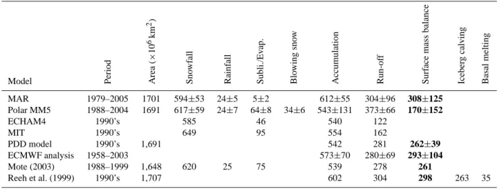
Table 1. Annual mass balance components simulated by MAR, Polar MM5 (Box et al., 2006), ECHAM4 and MIT models (Bugnion and Stone, 2002), a PDD model (Janssens and Huybrechts, 2000), derived from the ECMWF (re)analysis (Hanna et al., 2005), derived from SSM/I observations (Mote, 2003) and estimated by Reeh et al. (1999) which use in situ observations. The period over which it is averaged and the ice sheet area are also shown. Accumulation is calculated as snowfall plus rainfall minus erosion from the net water fluxes and the wind (blowing snow). Units are km3yr−1.
Model Period Area
(× 10 6km 2) Sno wf all Rainf all Subli./Ev ap. Blo wing sno w Accumulation Run-of f Surf ace mass balance Iceber g calving Basal melting MAR 1979–2005 1701 594±53 24±5 5±2 612±55 304±96 308±125 Polar MM5 1988–2004 1691 617±59 24±7 64±8 34±6 543±131 373±66 170±152 ECHAM4 1990’s 585 46 540 122 MIT 1990’s 649 95 554 162 PDD model 1990’s 1,691 542 281 262±39 ECMWF analysis 1958–2003 573±70 280±69 293±104 Mote (2003) 1988–1999 1,648 620 25 75 539 278 261 Reeh et al. (1999) 1990’s 1,707 602 304 298 263 35
a time step of 120 s. The ERA-40 reanalysis (1977–2002) and after that, the operational analysis (2002–2006) from the European Centre for Medium-Range Weather Forecasts (ECMWF) are used to initialize the meteorological fields at the beginning of the simulation in September 1977 and to force the lateral boundaries with temperature, specific hu-midity and wind components during the simulation. The (re)analysis is available every 6 h at a resolution of one de-gree (∼100 km). The Sea Surface Temperatures (SST) and the sea-ice extent in the SISVAT module are also prescribed by the reanalysis. No reinitialisations/corrections are applied to the model outputs. The schemes and set-up used here are fully described in Fettweis et al. (2005) and Lefebre et al. (2005).
3 Surface mass balance of the Greenland ice sheet
3.1 Average annual rates of the SMB components
3.1.1 Results
All the models listed in Table 1 agree unanimously to give an annual total ice sheet mass snowfall rate of ∼600 km3yr−1.
The net erosion by surface water vapour fluxes is estimated to be ∼50–100 km3yr−1(except by the MAR model) which
gives an accumulation rate (usually noted P-E) of approxi-matively 550 km3yr−1. The MAR simulated annual snowfall and net surface water vapour fluxes are respectively plotted in Figs. 1a and 2a. The MAR solid precipitation shows spa-tial patterns identified in interpolation of ice core and snow pit data (e.g., Ohmura et al., 1999; Cogley, 2004) or simu-lated by models (e.g., Hanna et al., 2002, 2006; Box et al.,
2006). See Fettweis et al. (2005) for more details about the validation of the MAR precipitation.
Unlike other models, the deposition/condensation accu-mulation simulated by MAR nearly dominates, in average, the sublimation/evaporation erosion over the whole ice sheet (see Table 1). Except at the summit where the small gain of mass modelled by MAR is consistent with the GC-Net obser-vations, MAR underestimates the mass loss resulting from sublimation/deposition by comparison with the Polar MM5 outputs (Box et al., 2006) and the Box and Steffen (2001) estimates based on GC-net observations (see Fig. 2a). This problem will be investigated in the future by reviewing the turbulence scheme used in the GrIS simulations with MAR.
The run-off is estimated to be ∼300 km3yr−1(except by the ECHAM4 and MIT models), which gives an estimation of the SMB around 300 km3yr−1when balancing the glacier discharge and basal melting rate as estimated by Reeh et al. (1999). Their glacier discharge estimation represents a min-imum value under current climatic conditions according to Box et al. (2006) because they do not account for the melt-induced outlet glacier acceleration observed by Zwally et al. (2002). The larger run-off rate simulated by the Polar MM5 model could be partly explained by the discrepancies in the used ice sheet mask i.e. in the classification of ice/land/ocean land surface type. Along the southeastern coast, the MM5 ice sheet margin runs directly along the coastline, which in-creases significantly the melt overall. Other ice sheet masks (Mote, 2003; Fettweis et al., 2005; Hanna et al., 2005) de-fine tundra grid points between the ice sheet margin (which lies at higher altitude as a result) and the sea. Besides, the MM5 SMB estimation is the only model taking into account snow erosion by the wind. The ECHAM4 and MIT models
24 X. Fettweis: The 1979–2006 Greenland ice sheet surface mass balance
Fig. 1. The 1979–2006 annual mean (left), 28-year linear regression change (centre) and autocorrelation (right) of the snowfall. Units are mm of water equivalent (mmWE) The autocorrelation is defined as the correlation between time series of the annual total ice sheet snowfall with that at each grid location. The autocorrelation shows where regional variability best captures the variability over the complete ice sheet. Under each plot, minimum and maximum values are indicated as well as the ice sheet average and the standard deviation.
Fig. 2. Same as Fig. 1 but for the net surface water vapour fluxes (i.e. the evaporation, condensation, sublimation and deposition).
underestimate the ablation rate due to the absence of run-off along the northern coast of the ice sheet according to Bugnion and Stone (2002).
While the MAR model underestimates the sublima-tion/evaporation mass loss, it is consistent with other mod-els by giving a SMB rate of 308 km3yr−1. In addition, the
Fig. 3. Same as Fig. 1 but for the SMB. The plot (a) shows the mean accumulation zone in red and the ablation zone in blue. The equilibrium zone, where the average SMB over the last 28 years is null, is plotted in white. The plot (c) shows that the melt variability in the (western) ablation zone influences more the SMB than the solid precipitation variability.
MAR patterns shown in Fig. 3a fully agree with other esti-mations based on both observations (Zwally and Giovinetto, 2001) and models (Box et al., 2004, 2006; Hanna et al., 2005) The MAR sublimation/evaporation underestimation can be assumed to be systematic each year. Therefore, it is reason-able to suppose that it weakly affects the temporal variability of the components simulation and that the MAR results can be used in a reliable way to study the SMB components evo-lution over the last 28 years. However, the accuracy of our model needs to be improved in the future to produce more reliable assessments of surface mass budget terms and their temporal changes.
3.1.2 Discussion
Contrary to Box et al. (2006) and Hanna et al. (2007) who calibrated SMB outputs during or after the simulation, the MAR outputs are not recalibrated and corrected. However, the use of remote sensing observations (as melt estimate from Tedesco, 2007) during the MAR simulation could im-prove our modelled SMB results. For example, remote data (albedo, liquid water content) easily detects the presence of bare ice/fresh snow in the ablation zone in summer. In the case of discrepancies between MAR and remote data, the MAR snow pack could be updated tracking down the pre-cise time, when bare ice appears in the ablation zone in sum-mer, has a great impact on the simulated SMB because of the albedo feedback (Lefebre et al., 2005). Applying these changes during the simulation (instead of after) allows the
model to take directly into account the feedback mechanisms of the bare ice apparition.
In addition, the modelled run-off could be validated with satellite derived observations (the run-off rate could be de-rived from changes in the snow pack liquid water content). The run-off rate differs for each model listed in Table 1. It constitutes the largest uncertainty in the current SMB esti-mations because no observations are available to validate this flux on which predicted sea level rise and THC perturbations depend. In the global warming context, this meltwater flux could change quickly and a good knowledge of its current behaviour is needed to make accurate projections in the fu-ture.
Finally, the model results for the GrIS SMB components (especially the run-off) vary quite a lot from one another. It is clear that some of the disagreements between the models come from biases within the models as well as from large dif-ferences in the processes resolved by the snow model and the coupling with the atmosphere: i) The MAR climate model has a complex snow model fully coupled with the atmo-spheric module running at the same resolution (i.e. 25 km); ii) The MM5 model used by Box et al. (2006) is an at-mospheric weather model running at a resolution of 24 km and it is coupled with a simplified snow model which takes however into account the blowing snow erosion (Snow pack properties in MM5 mainly derive from the direct measure-ments driving the model during simulation); iii) The Hanna et al. (2007) estimations use a complex snow model running
26 X. Fettweis: The 1979–2006 Greenland ice sheet surface mass balance
Fig. 4. Time series of the annual total ice sheet (a) SMB, (b) snowfall, (c) run-off, (d) net water vapour fluxes, (e) SMB averaged over the ice sheet area below 2000 m and (f) above 2000 m. Units are km3yr−1. The correlation with the whole ice sheet SMB is indicated as well as the trend. The linear trends are in km3yr−2.
at a resolution of 5 km forced by monthly mean atmospheric fields from the ECMWF (re)analysis available at a resolution of 110 km; iv) The Mote (2003) estimations use a Positive Degree Day (PDD) model at a resolution of 25 km forced by the SSM/I brightness temperature and by the Bromwich et al. (2001) accumulation time series. But, the used ice sheet mask, the resolution and the spin-up time could also be a cause of disagreement between models. Their impacts on the modelled SMB results should be investigated in the future:
– First, a too large ice sheet mask (i.e. with low-altitude
pixels, where there is no ice) leads to an overestima-tion of the run-off (as discussed in Sect. 3.1.1 for the MM5 results). A model with a too small ice sheet area will rather overestimate the SMB. In addition, due to the albedo feedback, biases in the ice sheet mask will also have an impact on the surface energy balance.
– Secondly, the resolution (and then the topography)
used in a model can significantly influence the simu-lated SMB because the ablation zone where substantial
seasonal melting occurs, is not wider than 100 km in Greenland. A too coarse resolution the model from re-solving adequately the steep ice sheet margin and the ablation zone. The resolution impacts also the precipi-tation (Fettweis et al., 2005).
– Thirdly, modelling results are very sensitive to the
spin-up time used in the snow model. At the beginning of the summer, the ice sheet and the tundra are covered by the winter snow accumulation. Either climatologic precip-itation data or reanalysis are used to initialize the snow model at the end of the spring, or the winter accumu-lation is simulated by the model itself by beginning the simulation at the end of the previous summer. Previous MAR simulations showed a very large sensitivity to the initial snow height and the snow properties above the tundra and the ablation zone given the albedo feedback (Lefebre et al., 2005). A too thick snow pack at the be-ginning of the summer above the ablation zone delays the appearance of bare ice (with a lower albedo) in the ablation zone and can considerably reduce the melting. That is why it is preferable to begin the simulation at the end of the previous summer (or several years be-fore) in order to reduce the problem of the snow model initialization. For example, let us quote the MAR model which uses a spin-up of 2–3 years while the surface in the MM5 model is reinitialised every day with a spin-up time of 6 hours due to the fact that MM5 is used in a forecast mode (Box et al., 2006). To reduce the impacts of the reinitialisation, MM5 is however driven by data (SMB measurements from the GC-Net Auto-matic Weather Stations and remote sensing derived sur-face albedo) independent of the ECMWF atmospheric analyses used to force the model at its boundaries.
3.2 Temporal variability and trend of the SMB components
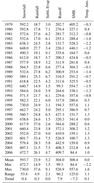
The SMB is governed, on the one hand by accumulation (snowfall) and on the other hand, by run-off (tempera-ture). The interannual variability in precipitation and abla-tion causes SMB fluctuaabla-tions (with a correlaabla-tion of respec-tively 0.71 and −0.90, see Fig. 4). In 1985, the SMB rate is abnormally low mainly because of low snowfall (see Ta-ble 2). Other SMB minima, rather due to a high freshwater flux into the ocean, are found in 1998 and 2003 in agree-ment with the Hanna et al. (2007) estimations. The abso-lute minimum of the SMB is reached in 2006 due to high run-off and very low snowfall. Maxima of SMB occur in two cases: in 1983 and 1992 after the volcanic eruptions from El Chichon and Mount Pinatubo that induced cool-ing and low meltcool-ing rates; in 1996, owcool-ing to both negative run-off and positive snowfall anomalies, the SMB reaches a positive record rate as in Hanna et al. (2007). Integrated over the ice sheet, the 28-year snowfall rate shows a posi-tive trend of +0.4±2.5 km3yr−2. The uncertainty range of
Table 2. Annual surface mass balance components (in km3yr−1) and annual temperature anomaly (in◦C yr−1).
Sno wf all Rainf all Subli./Ev ap. Runof f SMB Temp. Ano. 1979 592.2 18.7 3.0 202.7 405.2 −0.3 1980 592.8 17.8 7.1 276.4 327.1 0.4 1981 572.6 27.6 6.2 281.7 312.3 −0.8 1982 532.6 17.0 6.1 255.1 288.4 −1.0 1983 638.3 24.5 2.8 131.7 528.3 −2.2 1984 648.0 27.7 3.4 226.1 446.1 −1.2 1985 490.3 19.1 9.1 335.6 164.7 0.6 1986 612.0 18.7 5.7 200.3 424.8 −0.5 1987 577.9 18.9 3.2 311.9 281.8 0.4 1988 564.5 23.8 6.6 277.4 304.3 −0.1 1989 532.6 27.8 6.2 300.9 253.4 −1.4 1990 589.1 25.3 6.7 316.5 291.2 −0.7 1991 618.8 22.5 4.2 311.6 325.5 −0.5 1992 640.7 14.9 1.5 99.3 554.7 −1.9 1993 584.6 24.0 5.9 264.6 338.1 −1.3 1994 571.5 21.7 6.1 229.6 357.6 −0.8 1995 582.3 22.1 6.0 317.9 280.6 0.3 1996 730.0 24.9 3.1 194.3 557.6 1.1 1997 662.7 24.2 5.0 295.1 386.9 0.7 1998 560.7 24.8 6.5 427.3 151.7 1.3 1999 638.6 24.6 1.5 320.3 341.4 0.0 2000 617.9 37.6 2.6 364.6 288.2 0.6 2001 660.4 23.8 3.8 372.1 308.2 1.2 2002 552.0 27.0 9.0 410.9 159.1 1.3 2003 601.7 33.4 7.5 526.9 100.7 1.3 2004 579.4 28.3 5.8 442.9 159.0 0.9 2005 607.1 21.5 7.5 408.3 212.8 1.6 2006 472.7 26.1 4.7 409.7 84.4 1.0 Mean 593.7 23.9 5.2 304.0 308.4 0.0 Min 472.7 14.9 1.5 99.3 84.4 −2.2 Max 730.0 37.6 9.1 526.9 557.6 1.6 Range 53.4 4.9 2.1 96.2 125.0 1.1 Trend 0.4 0.3 0.0 7.9 −7.2 0.1
the snowfall trend (denoting two standard deviations of the trend i.e. a significance of 95%) indicates clearly that the trend is not significant according to Appendix A. The run-off increase is evaluated to be +7.9±3.3 km3yr−2 (with a
significance of 98%) which gives a global average sea level rise of (+2.2±0.9)×10−2mm yr−2. The computation was
made by using an area of a world ocean area of 361 mil-lion km2. As only the run-off increase is significant against the snowfall increase, the net effect of these competing fac-tors is a 95%-significant SMB mass loss rate, simulated to be
−7.2 km3yr−2with an uncertainty range of ±5.1 km3yr−2. The contribution of changes in net water vapour fluxes to the SMB variability is negligible (+0.02±0.1 km3yr−2), in
28 X. Fettweis: The 1979–2006 Greenland ice sheet surface mass balance
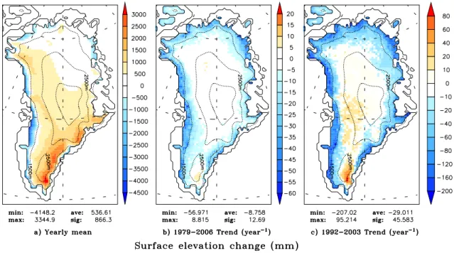
Fig. 5. Rates of elevation change (dS/dt) in cm yr−1for the 1992–2003 and the 1979–2006 periods. Only the changes due to the interannual variability of the snowfall, melt and water vapour fluxes are taken into account here. The topography (and consequently the margin glaciers) of the ice sheet is assumed to be constant during the simulation.
Table 3. Rates of surface elevation change (dS/dt) simulated by the MAR model, derived from ERS satellite radar altimeter data (Johannessen et al., 2005; Zwally et al., 2005), the NASA’s airborne (Airborne Topographic Mapper, ATM), and the satellite (ICEsat) laser altimeter surveys (Thomas et al., 2006). The period over which it is averaged is shown. Units are mm yr−1.
Data Period <1500 m ≥1500 m <2000 m ≥2000 m Total MAR model 1979–2006 −29±16 −15±27 −40±24 −4±20 −9±8 MAR model 1992–2003 −103±80 −44±120 −137±99 −10±83 −29±34 ERS data (Johannessen et al., 2005) 1992–2003 −20±9 +64±5 +25±7 +65±4 +54±2 ERS data (Zwally et al., 2005) 1992–2002 −56±14 +42±5 −14±12 +48±2 +27±3 ATM/ICEsat data (Thomas et al., 2006) 1993–2004 −257±30 +12±10 −153±17 +24±10 −45±11
agreement with Box et al. (2006). As shown in Fig. 4e and f, the heavier precipitation in the accumulation zone partly offsets the significant melt increase in the ablation zone. In-deed, the SMB variability shows an insignificant positive trend above 2000 m (+0.7±1.7 km3yr−2) against a signifi-cant negative trend of −7.8±4.0 km3yr−2below 2000 m.
Over the 1979–2006 (resp. 1992–2003) period, MAR simulates a GrIS mean surface elevation decrease of
−9±8 mm yr−1(resp. −29±34 mm yr−1). Only the eleva-tion change over 1979–2006 is 95%-significant according to Appendix A. Patterns are shown in Fig. 5 and changes simu-lated by MAR below/above 1500 m/2000 m are summarized in Table 3. Only the decreases below 1500/2000 m are sig-nificant. These results are fully consistent with recent obser-vations of surface elevation changes from satellite and
air-craft altimeter shown in Table 3 (Johannessen et al., 2005; Zwally et al., 2005; Thomas et al., 2006). Highest consis-tency is found with the last available observations derived estimations from Thomas et al. (2006) showing also a GrIS surface elevation decrease over the 1993–2004 period. Previ-ous ERS satellite radar altimeter estimates showing rather a GrIS elevation increase are not consistent with other studies (e.g. Velicogna and Wahr, 2005; Chen et al., 2006; Luthcke et al., 2006) and need therefore to be considered with caution as discussed by Thomas et al. (2006). In addition, the inter-annual variability is very important and a 12-year long data set is still too short to establish long-term trends.
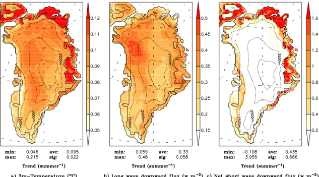
The melt increase occurs everywhere along the ice sheet margin (Fig. 6b) according to the GrIS warming shown in Fig. 7a. Warming is more pronounced above the ice sheet
Fig. 6. Same as Fig. 1 but for the available meltwater. Part of this meltwater is refrozen and does not reach the ocean (Lefebre et al., 2003).
Fig. 7. The 28-year linear regression change for the summer 3m-Temperature (left), for the summer downward infrared radiation (centre) and for the summer solar net radiation (right).
than along its margin, given that the surface temperature of melting snow/ice is limited to 0◦C. The higher positive snow-fall trend occurs near the south-eastern snowsnow-fall maximum (Fig. 1b) and negative trends are found along the ice sheet margin (lower in altitude). These negative trends are partly
explained by the warming, which causes an increase in the amount of liquid precipitations versus solid ones (Fig. 8b). These changes increase the meltwater supply and also impact glacier flow lubrication according to Zwally et al. (2002). Finally, Fig. 1c shows that the snowfall at Summit is an
30 X. Fettweis: The 1979–2006 Greenland ice sheet surface mass balance
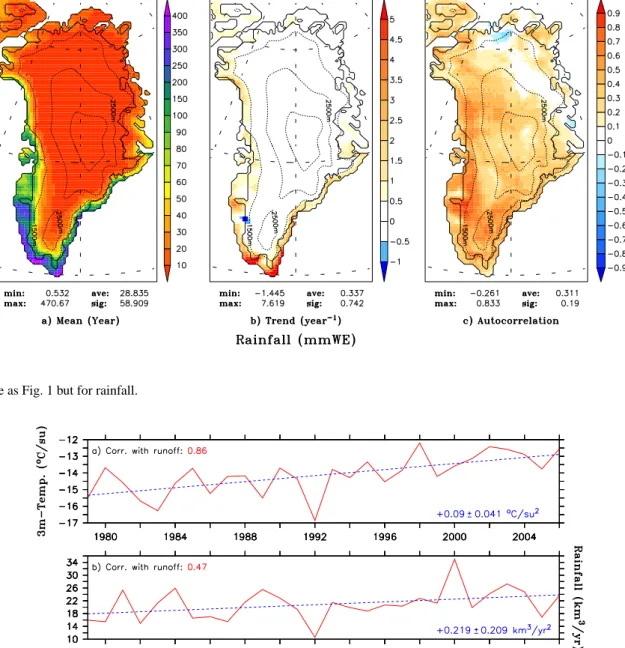
Fig. 8. Same as Fig. 1 but for rainfall.
Fig. 9. Time series of the total ice sheet (a) summer (from 1 May to 30 September) temperature average (in◦C su-1) and (b) yearly rainfall (in km3yr−1). The correlation with the run-off (Fig. 4) is indicated as well as the trend.
excellent indicator of the total ice sheet snowfall variabil-ity; this fully justifies the choice of this location for ice-core Greenland climate reconstructions. Given that the melt in-creases everywhere, positive trends in the SMB occur only in the extreme South of the GrIS where snowfall increases and dominates over ablation (Fig. 3b). MAR simulates negative 28-year SMB trends almost everywhere in the ablation zone (in red in Fig. 3a) and a significant positive SMB trend in the south-eastern of the GrIS. Figure 3c fully justifies SMB mea-surements near the K-Transect (in the south-western ablation
zone) as records of the total GrIS SMB variability (Greuell et al., 2001).
The summer temperature exhibits a robust correlation with the meltwater supply and therefore with the run-off (0.86) from the ice sheet as a whole (Fig. 9). This provides the basis for degree-day models. The occurrence of heavier rainfalls also increases the liquid water supply. It is a fact that the liquid fraction of the overall precipitation is increasing on the GrIS (+0.2±0.2 km3yr−2) but it does not explain more than 5% of the positive run-off 28-year trend estimated by
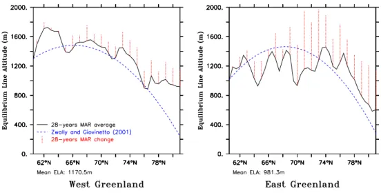
Fig. 10. Average equilibrium line altitude variations in MAR simulation (solid) and estimated by Zwally and Giovinetto (2001) parametriza-tion (dashed). The MAR 28-year changes are also shown (dotted).
Fig. 11. Time series of the winter (from 1 October YEAR-1 to 30 April YEAR) snowfall before the considered year (in km3yr−1) over (a) the ice sheet and (b) the tundra. The correlation with the SMB (Fig. 4) is indicated.
MAR (+7.9±3.2 km3yr−2). The large part of the run-off
acceleration is explained by the warming, estimated by MAR to be 0.09±0.04◦C yr−1. According to (Box et al., 2004), these considerations allow us to estimate the SMB anomaly for the entire ice sheet from the annual (yr) and June-July-August (JJA) temperature and the snowfall anomalies despite that these are not correlated. We have then:
1SMBGrIS= −64.771TGrISyr+1.571SFGrISyr (1)
1SMBGrIS= −69.361TGrISJJA+1.191SFGrISyr (2)
where 1SMBGrIS is the annual GrIS SMB anomaly in
km3, 1TGrISis the annual (resp. JJA) GrIS 3m-temperature
anomaly in K and 1SFGrIS is the annual GrIS
snow-fall anomaly in km3. The correlation (r) and the root mean square error (RMSE) between the SMB simulated anomaly and the SMB estimated anomaly are r=0.91 and RMSE=50.3 km3(resp. r=0.96 and RMSE=34.33 km3). Such correlations confirm our hypothesis about the acute sen-sitivity to the SMB to both temperature and snowfall anoma-lies. If we use only the JJA temperature (in K) and the annual snowfall anomalies (in mmWE) taken at Summit (the pixel used here has a latitude of 72.52◦N, a longitude of 38.50◦W and an altitude of 3232 m) to estimate the annual GrIS SMB
32 X. Fettweis: The 1979–2006 Greenland ice sheet surface mass balance
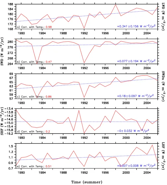
Fig. 12. For the whole ice sheet, time series of the mean summer (a) long wave downward flux (LWD), (b) short wave downward flux (SWD), (c) net short wave downward flux (SWDn), (d) sensible heat flux (SHF) and (e) latent heat flux (LHF). The correlation with the 3m-temperature (see Fig. 9) is indicated. Units are in W/m2.
anomaly (in km3),
1SMBGrIS= −73.291TSummitJJA+1.901SFSummityr (3)
the correlation remains very high (r=0.91 and RMSE=52.35 km3) which suggests that the records at Summit are very good proxies of the current SMB variabil-ity. Finally, the annual SMB (in mmWE) simulated near the JAR-1 automatic weather station (the pixel used here has a latitude of 69.33◦N, a longitude of 49.59◦W and an altitude of 734.1 m) shows a very good correlation with the annual GrIS SMB (in km3):
1SMBGrIS= −0.121SMBJAR−1yr (4)
where r=0.91 and RMSE=37.0 km3. Figure 3 shows the lo-cations quoted in the text.
3.3 The Equilibrium Line Altitude
The Equilibrium Line Altitude (ELA) is defined as the ele-vation where the SMB equals zero. Therefore, the ELA pro-vides an useful indicator of the combined influence of ther-mal and precipitation forcing on the SMB. Our results (see Fig. 10) are consistent with Zwally and Giovinetto (2001) parametrisation. The general pattern is obviously a lowering of the ELA with increasing latitude. Regional variation in the ELA versus latitude pattern results from changes in local topography and precipitation regimes due to the proximity or not of dominant cyclonic systems. The relatively weak ELA at 61◦N across the GrIC results, for example, from abundant snowfall observed in this region (see Fig. 1a). The
trends for these last 28 years is a positive shift of +4.9 m yr−1
(resp. +12.6 m yr−1) of the western (resp. eastern) Greenland
ELA. The positive shift of the ELA occurs everywhere (in red in Fig. 10) except at 62◦N in western Greenland which is the only region where the SMB is increasing (see Fig. 3b). These results corroborate the dominance of the thermal fac-tors variability on the SMB.
3.4 The albedo-temperature feedback
Mote (2003) suggests that high accumulation years are often associated with low ablation for the entire ice sheet due to the well-known albedo-temperature feedback. Low accumu-lation rates lead to more rapid losses of winter snow and to higher degree day factors for bare ice in the ablation zone. The thicker the snow pack at the end of spring, the later the bare ice (with a lower albedo) appears (Fettweis et al., 2005). A good example of the hypothesis of Mote (2003) is 1996 (see Table 2) but Fig. 11 reveals however that this hypothesis does not explain the SMB variations of these last 28 years. Indeed, the winter snow accumulation has not significantly changed while the SMB variability suggests a negative trend. As already explained, we have found that the thermal factors dominate currently the SMB sensitivity rather than the pre-cipitation changes. These last results confirm our assump-tion.
4 Surface energy balance of the Greenland ice sheet
Since 1979, the SMB has been decreasing due to increas-ing run-off rates explained by higher temperatures. Only the increase of the long wave downward (LWD) flux and the de-crease of surface albedo can explain this warming as shown in Fig. 12. No significant change occurs in both sensible and latent heat fluxes since 1979. The short wave downward (SWD) flux interannual fluctuations are very weak during the last 28 years except the negative anomalies in 1983 and 1992 due to the eruption of El Chich˜on and Mount Pinatubo, re-spectively (Hanna et al., 2005). These volcanic eruptions in-jected large amounts of aerosols in the atmosphere; this re-duced the amount of solar energy reaching the Earth surface. Therefore, the net solar radiation (SWDn=SWD×[1−α]) has been increasing due to a decrease of the surface albedo (α). Increased melting undoubtedly reduces the surface albedo, which then obviously amplifies the warming-related melt in-crease. This amplification is particularly visible in the North-East Greenland tundra where the snow cover has been disap-pearing earlier in the summer these last years (see Fig. 7). In the previous section, we have shown that the winter ac-cumulation variability can not explain the albedo variabil-ity; Fig. 13 confirms that the albedo decrease over the 1979– 2006 period starts after the middle of the summer in the tun-dra due to higher temperatures. Therefore, it seems reason-able to conclude that SWDn changes are primarily driven by
Fig. 13. Time series of the average tundra albedo for April, May, June, July and August. The 1979–2006 linear trend is dotted.
the melt increase and, to a lesser extent, by the rainfall in-crease which humidifies the snow pack and reduces the sur-face albedo (Fig. 8). Consequently, only the positive LWD tendency leads to the overall warming of the ice sheet sur-face. The net solar radiation increase is besides restricted to the ablation zone and the tundra while the infrared radiation, as well as the 3m-temperature, have been increasing every-where. The temperature is obviously better correlated with the infrared radiation than with the solar net radiation as can be seen in Fig. 14.
5 The North Atlantic Oscillation
The North Atlantic Oscillation (NAO) represents the domi-nant mode of regional atmospheric variability around Green-land (e.g. Rogers, 1997; Appenzeller et al., 1998; Bromwich et al., 1999) and is gauged here by the NAO index, which is computed as the normalised pressure difference between Gibraltar minus Reykjavik (Jones et al., 1997; Osborn, 2004). It is closely related to the Arctic Oscillation (AO) (Thompson et al., 1998) and is one of the major modes of variability of the Northern Hemisphere atmosphere, partic-ularly in winter. Moreover, a large fraction of the climate changes observed during the last decades in the Arctic could be related to the positive trend in the NAO/AO index dur-ing this period (e.g., Rigor et al., 2000; Moritz et al., 2003; Hanna and Cappelen, 2003; Rogers et al., 2004; Johannessen et al., 2005). The NAO is characterized by a dipole of sur-face pressure between mid- and high-latitudes, resulting in changes in the strength of the westerly winds at mid-latitudes
34 X. Fettweis: The 1979–2006 Greenland ice sheet surface mass balance
Fig. 14. Correlation coefficient in the summer between the 3m-temperature and the infrared radiation (left) and the net solar radiation (right), respectively. The correlation coefficient is computed by using the annual time series of each pixel.
Fig. 15. Seasonal temperature sensitivity of the Greenland ice sheet to the NAO. Only correlation coefficients above 0.3 are significant. The maps represents from left to right: the annual, winter (DJF), spring (MAM), summer (JJA) and autumn (SON) mean. The source of the NAO index comes from the Climate Research Unit (CRU), at http://www.cru.uea.ac.uk/cru/data/nao.htm.
and large winter temperature variations. A positive NAO phase shows a stronger than usual subtropical high pres-sure centre and a deeper than normal Icelandic low. The
increased pressure difference results in more numerous and stronger winter storms crossing the Atlantic Ocean on a more northerly track. This results in warm and wet winters in
Fig. 16. Same as Fig. 15 but for precipitation (solid and liquid).
Europe and in cold and dry winters in northern Canada and Greenland.
According to recent observations from Johannessen et al. (2005), the maximum of the GrIS sensitivity to the NAO vari-ability is found in winter (DJF) (Table 4). The temperature (via the long wave radiations) is the most sensitive compo-nent and is significantly anti-correlated to the NAO as already pointed out by Chylek et al. (2004). When the NAO index is negative, the location of the Icelandic low favours (southerly) warm air advection along the southwest coast of Greenland and over the ice sheet. This explains why the temperature correlation with the NAO is maximum in the south(west) of Greenland (Fig. 15). Everywhere and during every sea-son, the temperature is anti-correlated to the NAO although this correlation is not significant in summer (JJA), in par-ticular along the northeastern coast as found by Chylek and Lohmann (2005).
Modelled precipitation variability also presents significant links with the NAO (Fig. 16). Consistent with the regional temperature sensitivity, a positive NAO phase (i.e. cold win-ter) is associated with less precipitation in the southeast in winter (DJF) and autumn (SON). Generally, when the NAO is positive, stronger westerlies reduce the southwesterly flow that brings moisture to Greenland, resulting in an average re-duction of the snow accumulation. On the contrary, when the NAO is negative, the large-scale atmospheric flow is more frequently from the southwest bringing more moisture to the ice sheet, particularly in the southern region (Mosley-Thompson et al., 2005). Except in summer (JJA), the sim-ulation reflects very well the heavier precipitation along the ice sheet eastern slope and the diminished precipitation along the western slope during high NAO phases. This pattern has been also identified by Appenzeller et al. (1998). Significant
Table 4. Mean Greenland ice sheet sensitivity to the NAO for the 1979–2006 period. The source of the North Atlantic Oscillation (NAO) index is the Climate Research Unit (CRU), at http://www. cru.uea.ac.uk/cru/data/nao.htm. W inter (DJF) Spring (MAM) Summer (JJ A) Autumn (SON) Y ear Precipitation −0.42 −0.32 0.18 −0.33 −0.13 3m-Temperature −0.76 −0.45 −0.23 −0.56 −0.67
positive correlations with the NAO are obvious in summer (JJA) in the northwest and in the east.
The temperature is anti-correlated with the NAO index ev-erywhere and in every season; up to half of the temperature variability is explained by the NAO in winter (DJF). In sum-mer (JJA), the sensitivity to the NAO is not significant (Ta-ble 4) in agreement with Hanna et al. (2007). Some NAO links with precipitation can also be found but they are less homogeneous in time and space. In an annual average and averaged over the ice sheet, the precipitation is not correlated with the NAO as in Hanna et al. (2006). Therefore the NAO is a good proxy for the Greenland winter temperature but does not explain the accumulation (winter snowfall) nor the melt (summer temperature) changes over the last 28 years. Beside, the last 40 years are characterized by large positive trends of NAO/AO indexes (Solomon et al., 2007) suggest-ing rather a coolsuggest-ing in Greenland and a warmsuggest-ing in the Arc-tic region (Hanna and Cappelen, 2003; Goosse and Holland, 2005).
36 X. Fettweis: The 1979–2006 Greenland ice sheet surface mass balance
Fig. 17. Time series of run-off evolution for Greenland divided in 5 regions. The regions boundaries are −44◦N in longitude and 70◦N and 80◦N respectively in latitude. The run-off rates presented here include freshwater fluxes from both ice sheet and tundra.
6 Discussion and conclusions
A 28-year simulation (1979–2006) of the GrIS shows an insignificant increase in solid precipitation (+0.4±2.5 km3yr−2) but a significant and positive pertur-bation of the meltwater production (+7.9±3.3 km3yr−2). The increasing snowfall offsets the run-off increase to give a significant SMB mass loss rate of −7.2±5.1 km3yr−2. The contribution of changes in the net water vapour fluxes to the SMB variability is negligible (+0.02±0.09 km3yr−2). The meltwater production has increased because the GrIS surface has been warming up by +2.4◦C since 1979. More than 96% variance in the modelled surface mass balance total is explained by the summer (from 1 June to 31 August) temperature and the annual precipitation variability. A small part of the increasing liquid water supply comes from heavier rainfall (+0.2±0.2 km3yr−2). Due to higher temperatures, the liquid fraction of total precipitation has been increasing. Snowfall shows negative trends along the ice sheet margin where the amount of liquid precipitation has been increasing. The temperature has increased because of higher net solar and infrared radiations. No significant changes in either latent or sensible heat fluxes occur. The SWD flux does not show variations during these 28 years except negative anomalies in 1983 and 1992 due to volcanic eruptions (El Chich˜on and Mount Pinatubo). The SWDn flux has increased because the albedo has been decreasing. Lower accumulation rates in winter could explain this. Indeed, thin snow packs by the end of the winter lead to faster losses of winter snow mass and to higher degree day factors (i.e. higher solar radiation absorbed by the surface) for bare ice (with a lower albedo) in the ablation zone. But according to our results, winter snowfall has not changed. Therefore, it is rather resulting from the increasing melt which wets the snow and decreases the albedo. Besides, the SWDn flux has increased only in the zone where melting
has increased while the warming is occurring everywhere on the ice sheet. It is clear however that the decreasing albedo amplifies in turn the warming-related melt increase by the well-known albedo-temperature positive feedback. Consequently, the GrIS warming is mainly explained by higher LWD fluxes. The warming is almost uniform over the ice sheet as infrared radiations increase, suggesting that it comes from an external forcing.
The melt has significantly increased because the GrIS has been warming up at the surface in the last decades due to higher LWD fluxes. These changes are significant and can not be explained by natural variability (e.g. the North At-lantic Oscillation). Therefore, they could be a response (in agreement with the conclusions of Hanna et al., 2007) to the GHG concentration increase induced by human activ-ities since the beginning of the industrial era and the re-cent global warming related to it (Solomon et al., 2007). Higher GHG concentrations increase the incoming infrared fluxes and warm up the free atmosphere. Although the MAR radiative scheme includes the interannual fluctuations of gases/aerosols concentrations, the major temporal variabil-ity comes from its boundaries via the ECMWF (re)analysis which take into account the recent GHG concentration in-crease and the resulting global warming. The MAR sim-ulated 500 hPa-temperature is 0.98 correlated with the one obtained by the (re)anlaysis and that shows an increase of
+0.07◦C yr−1since 1979. Finally, the correlation between the annual MAR 3m-temperature averaged on the GrIS and the global average temperature from the CRU data set (Bro-han et al., 2006) is 0.66.
Since 1979, MAR simulates an increase of 102% of the freshwater flux into the ocean due to an acceleration of snow/ice melting at the GrIS surface. This increase oc-curs everywhere along the Greenland coast. Its maximum is found along the West coast (see Figs. 17 and 18). In-tegrated over Greenland (ice sheet and tundra), the 28-year
run-off rate shows a positive trend of +8.2±3.5 km3yr−2
which is equivalent to a rate of global average sea level rise of +2.3±1.0×10⁻²mm yr−2. The 28-year average of
the annual Greenland run-off is 407.2 km3yr−1 (sea level equivalent is +113×10−2mm yr−1). This flux reached 636.8 km3yr−1=2.02×10⁻²Sv in the melt record year of 2003. We must add to this flux the glacier discharge and the basal melting flux which is normally considered as equal to the meltwater flux. Furthermore, increases in meltwa-ter amount suggest an increase in glacier discharge duo to the observed meltwater-induced ice sheet flow acceleration (Zwally et al., 2002). Once the ice starts to melt at the sur-face, lakes develop and ultimately discharge into crevasses down to the glacier base. Meltwater lubricates this base and, doing so, impacts glacier movement.
To conclude, this paper shows that the GrIS has been sig-nificantly losing mass since the beginning of eighties, by an increasing meltwater run-off as well as by a probable increased iceberg discharge into the ocean due the process found by Zwally et al. (2002). The global warming induced by human activities could explain these changes. As a result, it seems that increased melting dominates over increased ac-cumulation in a warming scenario and that the GrIS will continue to lose mass in the future. The GrIS melting will have an effect on the stability of the thermohaline circula-tion (THC) and the global sea level rise. On the one hand, increases in the freshwater flux from the GrIS (glacier dis-charge and run-off) could perturb the THC by reducing the density contrast driving it. On the other hand, a melting of the whole GrIS would account for a global mean sea level rise of 7.4 m.
Appendix A
Uncertainty range given for the trend
The uncertainty range given for the trend of the SMB, run-off, . . . (plotted in Fig. 4) denotes two standard trend devia-tions (i.e. a significance of 95%) using the method described in Chapter 6.2 from Snedecor and Cochran (1971). It is com-puted from the time series plotted in Fig. 4 according to:
e1= X i (trend(ai) − ai)2 (A1) e2= X i (yi−mean(yi))2 (A2) range =pe1/((2006 − 1979 − 1) ∗ e2) ∗ k (A3) where
ai = time series of the variables plotted in Fig. 4
yi = time series of the 28 years (1979, 1980, . . .)
k=1.96 to have a significant of 95%. (k=1 or k=3 for a 67%
significant or a 99.5% significant respectively). The trend of
Fig. 18. Freshwater flux into the ocean in 2003 produced by melt-water run-off and rainfall. The freshmelt-water fluxes have been ob-tained by a routing scheme using the MAR topography. The routing scheme is a simplified version of the Multiple Path Distributed Flow Algorithm (see http://www.awi-bremerhaven.de/ATM/asood/route. html). It discharges the meltwater flux from each pixel to the pix-els at a lower altitude until the flux reaches the ocean. The routing scheme is run after the MAR simulation and consequently, no in-teraction of the meltwater coming from the higher-altitude pixels with the surface of the pixel (percolation, decrease of albedo, . . .) is taken into account. Finally, the distribution of meltwater flux lower-altitude pixels is lower-altitude-weighted. Units are 10−4Sv.
a time series is significant if it is higher than its uncertainty range.
Acknowledgements. All major computations were realized with the computing resources of the Institut de Calcul Intensif et Stokage de Masse (CSIM) from the Universit´e catholique de Louvain (http://www.cism.ucl.ac.be). The author would like to thank sincerely J.-P. van Ypersele for providing facilities during the writing of this paper. The comments and support from H. Gall´ee, M. Erpicum, J.-P. van Ypersele, F. Lefebre, W. Lefebvre were extremely valuable. Finally, the author also want to thank A. Prick for her precious spelling check in this manuscript.
38 X. Fettweis: The 1979–2006 Greenland ice sheet surface mass balance
References
Alley, R. B., Clark, P. U., Huybrechts, P., and Joughin, I.: Ice sheet and sea-level changes, Science, 310, 456–460, 2005.
Appenzeller, C., Schwander, J., Sommer, S., and Stocker, T. F.: The North Atlantic Oscillation and its imprint on precipitation and ice accumulation in Greenland, Geophys. Res. Lett., 25(11), 1939– 1942, 1998.
Box, J. E. and Steffen, K.: Sublimation estimates for the Green-land ice sheet using automated weather station observations, J. Geophys. Res., 106(D24), 33 965–33 982, 2001.
Box, J. E. and Rinke, A.: Evaluation of Greenland ice sheet surface climate in the HIRHAM regional climate model, J. Climate, 16, 1302–1319, 2003.
Box, J. E., Bromwich, D. H., and Bai, L.-S.: Greenland ice sheet surface mass balance for 1991–2000: application of Polar MM5 mesoscale model and in-situ data, J. Geophys. Res., 109(D16), D16105, doi:10.1029/2003JD004451, 2004.
Box, J. E., Bromwich, D. H., Veenhuis, B. A., Bai, L.-S., Stroeve, J. C., Rogers, J. C., Steffen, K., Haran, T., and Wang, S.-H.: Green-land ice sheet surface mass balance variability (1988–2004) from calibrated Polar MM5 output, J. Climate, 19(12), 2783–2800, 2006.
Box, J. E. and Cohen, A. E.: Upper-air temperatures around Greenland: 1964–2005, Geophys. Res. Lett., 33, L12706, doi:10.1029/2006GL025723, 2006.
Brohan, P., Kennedy, J. J., Haris, I., Tett, S. F. B., and Jones, P. D.: Uncertainty estimates in regional and global observed tempera-ture changes: a new dataset from 1850, J. Geophys. Res., 111, D12106, doi:10.1029/2005JD006548, 2006.
Bromwich, D. H., Chen, Q. S., Li, Y. F., and Cullather, R. I.: Pre-cipitation over Greenland and its relation to the North Atlantic Oscillation, J. Geophys. Res., 104(D18), 22 103–22 115, 1999. Bromwich, D. H., Chen, Q., Bai, L., Cassano, E. N., and Li, Y.:
Modelled precipitation variability over the Greenland ice sheet, J. Geophys. Res., 106, 33 891–33 908, 2001.
Brun, E., David, P., Sudul, M., and Brunot, G.: A numerical model to simulate snowcover stratigraphy for operational avalanche forecasting, J. Glaciol., 38, 13–22, 1992.
Bugnion, V. and Stone, P. H.: Snowpack model estimates of the mass balance of the Greenland ice sheet and its changes over the twenty first century, Clim. Dyn., 20, 87–106, 2002.
Chen, J. L., Wilson, C. R., and Tapley, B. D.: Satellite Gravity Mea-surements Confirm Accelerated Melting of Greenland Ice Sheet, Science, 313, 1958–1960, doi:10.1126/science.1129007, 2006. Chylek, P., Box, J. E., and Lesins, G.: Global Warming and the
Greenland Ice Sheet, Climatic Change, 63, 201–221, 2004. Chylek, P. and Lohmann, U.: Ratio of the Greenland to global
temperature change: Comparison of observations and cli-mate modeling results, Geophys. Res. Lett., 32, L14705, doi:10.1029/2005GL023552, 2005.
Chylek, P., Dubey, M. K., and Lesins, G.: Greenland warming of 1920–1930 and 1995–2005, Geophys. Res. Lett., 33, L11707, doi:10.1029/2006GL026510, 2006.
Cogley, J. G.: Greenland accumulation: An error model, J. Geo-phys. Res., 109, D18101, doi:10.1029/2003JD004449, 2004. De Ridder, K. and Gall´ee, H.: Land surface-induced regional
cli-mate change in Southern Israel, J. Appl. Meteorol., 37, 1470– 1485, 1998.
Dethloff, K., Schwager, M., Christensen, J. H., Kiilsholm, S.,
Rinke, A., Dorn, W., Jung-Rothenh¨ausler, F., Fischer, H., Kipf-stuhl, S., and Miller, H.: Recent Greenland accumulation esti-mated from regional model simulations and ice core ananlysis, J. Climate, 15, 2821–2832, 2002.
Dowdeswell, J.: The Greenland Ice Sheet and Global Sea-Level Rise, Science, 311(5763), 963–964, doi:10.1126/science.1124190, 2006.
Fettweis, X., Gall´ee, H., Lefebre, L., and van Ypersele, J.-P.: Greenland surface mass balance simulated by a regional cli-mate model and comparison with satellite derived data in 1990– 1991, Clim. Dyn., 24, 623–640, doi:10.1007/s00382-005-0010-y, 2005.
Fettweis, X., Gall´ee, H., Lefebre, L., and van Ypersele, J.-P.: The 1988–2003 Greenland ice sheet melt extent by passive mi-crowave satellite data and a regional climate model, Clim. Dyn., 27(5), 531–541, doi:10.1007/s00382-006-0150-8, 2006. Fettweis, X., van Ypersele, J.-P., Gall´ee, H., Lefebre, F., and
Lefeb-vre, W.: The 1979–2005 Greenland ice sheet melt extent from passive microwave data using an improved version of the melt retrieval XPGR algorithm, Geophys. Res. Lett., 34, L05502, doi:10.1029/2006GL028787, 2007.
Gall´ee, H. and Schayes, G.: Development of a three-dimensional meso-γ primitive equations model, Mon. Wea. Rev., 122, 671– 685, 1994.
Gall´ee, H., Guyomarc’h, G., and Brun, E.: Impact of the snow drift on the Antarctic ice sheet surface mass balance: possible sensi-tivity to snow-surface properties, Boundary-Layer Meteorol., 99, 1–19, 2001.
Goosse, H. and Holland, M.: Mechanisms of decadal Arctic vari-ability in the Community Climate System Model CCSM2, J. Cli-mate, 18(17), 3552–3570, 2005.
Greuell, W., Denby, B., van de Wal, R. S. W., and Oerlemans, J.: Ten years of mass balance measurements along a transect near Kangerlussuaq, Greenland, J. Glaciol., 47, 157–158, 2001. Hanna, E., Huybrechts, P., and Mote, T.: Surface mass
bal-ance of the Greenland ice sheet from climate analysis data and accumulation/run-off models, Ann. Glaciol., 35, 67–72, 2002. Hanna, E. and Cappelen, J.: Recent cooling in coastal southern
Greenland and relation with the North Atlantic Oscillation, Geo-phys. Res. Lett., 30, 1132, doi:10.1029/2002GL015797, 2003. Hanna, E., Huybrechts, P., Janssens, I., Cappelen, J., Steffen,
K., and Stephens, A.: Runoff and mass balance of the Green-land ice sheet: 1958–2003, J. Geophys. Res., 110, D13108, doi:10.1029/2004JD005641, 2005.
Hanna, E., McConnell, J., Das, S., Cappelen, J., and Stephens, A.: Observed and modeled Greenland ice sheet snow accumulation, 1958–2003, and links with regional climate forcing, J. Climate, 19, 344–358, 2006.
Hanna, E., Huybrechts, P., Steffen, K., Cappelen, J., Huff, R., Shu-man, C., Irvine-Fynn, T., Wise, S., and Griffiths, M.: Increased runoff from melt from the Greenland Ice Sheet: a response to global warming, J. Climate, in press, 2007.
Howat, I. M., Joughin, I. Tulaczyk, S., and Gogineni, S.: Rapid re-treat and acceleration of Helheim Glacier, east Greenland, Geo-phys. Res. Lett., 32, L22502, doi:10.1029/2005GL024737, 2005. Howat, I. M., Joughin, I., and Scambos, T. A.: Rapid Changes in Ice Discharge from Greenland Outlet Glaciers, Science, 315(5818), 1559, doi:10.1126/science.1138478, 2007.
re-tention in mass-balance parameterizations of the Greenland ice sheet, Ann. Glaciol., 31, 133–140, 2000.
Johannessen, O. M., Khvorostovsky, K., Miles, M. W., and Bobylev, L. P.: Recent ice sheet growth in the interior of Greenland, Sci-encexpress, 1013–1016, doi:10.1126/science.1115356, 2005. Jones, P. D., Jonsson, T., and Wheeler, D.: Extension to the North
Atlantic Oscillation using early instrumental pressure observa-tions from Gibraltar and South-West Iceland, Int. J. Climatol., 17, 1433–1450, 1997.
Krabill, W., Frederick, E., Manizade, S., Martin, C., Sonntag, J., Swift, R., Thomas, R., Wright, W., and Yngel, J.: Rapid thinning of parts of the southern Greenland ice sheet, Science, 283, 1522– 1524, 1999.
Krabill, W., Abdalati, W., Frederick, E., Manizade, S., Martin, C., Sonntag, J., Swift, R., Thomas, R., Wright, W., and Yungel, J.: Greenland Ice Sheet: High-Elevation Balance and Peripheral Thinning, Science, 289, 428–430, 2000.
Krabill, W., Hanna, E., Huybrechts, P., Abdalati, W., Cappelen, J., Csatho, B., Frederick, E., Manizade, S., Martin, C., Sonntag, J., Swift, R., Thomas, R., and Yungel, J.: Greenland Ice Sheet: Increased coastal thinning, Geophys. Res. Lett., 31, L24402, doi:10.1029/2004GL021533, 2004.
Lefebre, F., Gall´ee, H., van Ypersele, J., and Greuell, W.: Mod-eling of snow and ice melt at ETH-camp (west Greenland): a study of surface albedo, J. Geophys. Res., 108(D8), 4231, doi:10.1029/2001JD001160, 2003.
Lefebre, F., Fettweis, X., Gall´ee, H., van Ypersele, J., Marbaix, P., Greuell, W., and Calanca, P.: Evaluation of a high-resolution regional climate simulation over Greenland, Clim. Dyn., 25, 99– 116, doi:10.1007/s00382-005-0005-8, 2005.
Lemke, P., Ren, J., Alley, R. B., Allison, I., Carrasco, J., Flato, G., Fujii, Y., Kaser, G., Mote, P., Thomas, R. H., and Zhang, T.: Observations: Changes in Snow, Ice and Frozen Ground, in: Climate Change 2007: The Physical Science Basis, Contribution of Working Group I to the Fourth Assessment Report of the In-tergovernmental Panel on Climate Change, edited by: Solomon, S., Qin, D., Manning, M., Chen, Z., Marquis, M., Averyt, K. B., Tignor, M., and Miller, H. L., Cambridge University Press, Cambridge, United Kingdom and New York, NY, USA, 2007. Luckman, A. and Murray, T.: Seasonal variation in velocity before
retreat of Jakobshavn Isbræ, Greenland, Geophys. Res. Lett., 32, L08501, doi:10.1029/2005GL022519, 2005.
Luckman, A., Murray, T., de Lange, R., and Hanna, E.: Rapid and synchronous ice-dynamic changes in East Greenland, Geophys. Res. Lett., 33, L03503, doi:10.1029/2005GL025428, 2006. Luthcke, S. B., Zwally, H. J., Abdalati, W., Rowlands, D. D., Ray,
R. D., Nerem, R. S., Lemoine, F. G., McCarthy, J. J., and Chinn, D. S.: Recent Greenland Ice Mass Loss by Drainage System from Satellite Gravity Observations, Science, 314(5803), 1286, doi:10.1126/science.1130776, 2006
Mosley-Thompson, E., Readinger, C. R., Craigmile, P., Thompson, L. G., and Calder, C. A.: Regional sensitivity of Greenland pre-cipitation to NAO variability, Geophys. Res. Lett., 32, L24707, doi:10.1029/2005GL024776, 2005.
Moritz, R. E., Bitz, C. M., and Steig, E. J.: Dynamics of recent climate change in the Arctic, Sciences, 297, 1497–1502, 2003. Mote, T. L.: Estimation of runoff rates, mass balance, and
elevation changes on the Greenland ice sheet from passive microwave observations, J. Geophys. Res., 108(D2), 4056,
doi:10.1029/2001JD002032, 2003.
Ohmura, A., Calanca, P., Wild, M., and Anklin, M.: Precipitation, accumulation, and mass balance of the Greenland ice sheet, Zeit. Gletsch. Glazialgeol., 35, 1–20, 1999.
Osborn, T. J.: Simulating the winter North Atlantic Oscillation: the roles of internal variability and greenhouse gas forcing, Clim. Dyn., 22, 605–623, 2004.
Rahmstorf, S., Crucifix, M., Ganopolski, A., Goosse, H., Ka-menkovich, I., Knutti, R., Lohmann, G., Marsh, R., Mysak, L. A., Wang, Z., and Weaver, A. J.: Thermohaline circulation hys-teresis: A model intercomparison, Geophys. Res. Lett., 32(23), L23605, doi:10.1029/2005GL023655, 2005.
Reeh, N., Mayer, C., Miller, H., Thomson, H. H., and Weidick, A.: Present and past climate control on fjord glaciations in Green-land: Implications for IRD-deposition in the sea, Geophys. Res. Lett., 26, 1039–1042, 1999.
Ridley, J., Huybrechts, P., Gregory, J., and Lowe, J.: Future changes in the Greenland ice sheet: A 3000 year simulation with a high resolution ice sheet model interactively coupled to an AOGCM, J. Climate, 18, 3409–3427, 2005.
Rignot, E., Braaten, D., Gogineni, S. P., Krabill, W. B., and McConnell, J. R.: Rapid ice discharge from south-east Greenland glaciers, Geophys. Res. Lett., 31, L10401, doi:10.1029/2004GL019474, 2004.
Rignot, E. and Kanagaratnam, P.: Changes in the Velocity Structure of the Greenland Ice Sheet, Science, 311, 986–990, doi:10.1126/science.112138, 2006.
Rigor, I. G., Wallace, J. M., and Colony, R. L.: Response of sea ice to the Arctic Oscillation, J. Climate, 15, 2648–2663, 2000. Rogers, J. C.: North Atlantic storm track variability and its
associ-ation to the North Atlantic Oscillassoci-ation and climate variability of Northern Europe, J. Climate, 10(7), 1635–1647, 1997.
Rogers, J. C., Wang, S. H., and Bromwich, D. H.: On the role of the NAO in recent northeastern Atlantic Arctic warming, Geophys. Res. Lett., 31, L02201, doi:10.1029/2003GL018728, 2004. Snedecor, G. W. and Cochran, W. G.: M´ethodes statistiques,
Origi-nal Title: Statistical Methods 6th edition by The Iowa State Uni-versity Press, Ames, Iowa, USA, 67-21577, traduit par: Boelle, H. et Camhaji, E., Association de Coordination Technique Agri-cole, Paris, 649 pp, 1971.
Solomon, S., Qin, D., Manning, M., Alley, R. B., Berntsen, T., Bindoff, N. L., Chen, Z., Chidthaisong, A., Gregory, J. M., Hegerl, G. C., Heimann, M., Hewitson, B., Hoskins, B. J., Joos, F., Jouzel, J., Kattsov, V., Lohmann, U., Matsuno, T., Molina, M., Nicholls, N., Overpeck, J., Raga, G., Ramaswamy, V., Ren, J., Rusticucci, M., Somerville, R., Stocker, T. F., Whetton, P., Wood, R. A., and Wratt, D.: Technical Summary, in: Climate Change 2007: The Physical Science Basis, Contribution of Working Group I to the Fourth Assessment Report of the Intergovern-mental Panel on Climate Change, edited by: Solomon, S., Qin, D., Manning, M., Chen, Z., Marquis, M., Averyt, K. B., Tignor, M., and Miller, H. L., Cambridge University Press, Cambridge, United Kingdom and New York, NY, USA, 2007.
Tedesco, M.: Snowmelt detection over the Greenland ice sheet from SSM/I brightness temperature daily variations, Geophys. Res. Lett., 34, L02504, doi:10.1029/2006GL028466, 2007.
Thomas, R., Csatho, B., Davis, C., Kim, C., Krabill, W., Manizade, S., McConnell, J., and Sonntag, J.: Mass balance of higher-elevation parts of the Greenland ice sheet, J. Geophys. Res.,
40 X. Fettweis: The 1979–2006 Greenland ice sheet surface mass balance
106(D24), 33707, doi:10.1029/2001JD900033, 2001.
Thomas, R., Frederick, E., Krabill, W., Manizade, S., and Martin, C.: Progressive increase in ice loss from Greenland, Geophys. Res. Lett., 33, L10503, doi:10.1029/2006GL026075, 2006. Thompson, D. W. J. and Wallace, J. M.: The Arctic Oscillation
signature in the wintertime geopotential height and temperature fields, Geophys. Res. Lett., 9, 1297–1300, 1998.
Velicogna, I. and Wahr, J.: Greenland mass balance from GRACE, Geophys. Res. Lett., 32, L18505, doi:10.1029/2005GL023955, 2005.
Zwally, J. H. and Giovinetto, M. B.: Balance mass flux and ice ve-locity across the equilibrium line in drainage systems of Green-land, J. Geophys. Res., 106, 33 717–33 728, 2001.
Zwally, J. H., Abdalati, W., Herring, T., Larson, K., Saba, J., and Steffen, K.: Surface Melt-Induced Acceleration of Greenland Ice-Sheet Flow, Science, 297, 218–222, 2002.
Zwally, J. H., Giovinetto, M., Li, J., Cornejo, H., Beckley, M., Bren-ner, A., Saba, J., and Yi, D.: Mass changes of the Greenland and Antarctic ice sheets and shelves and contributions to sea-level rise: 1992–2002, J. Glaciol., 51(175), 509–527(19), 2005.