HAL Id: hal-03191695
https://hal.archives-ouvertes.fr/hal-03191695
Submitted on 7 Apr 2021
HAL is a multi-disciplinary open access
archive for the deposit and dissemination of
sci-entific research documents, whether they are
pub-lished or not. The documents may come from
teaching and research institutions in France or
abroad, or from public or private research centers.
L’archive ouverte pluridisciplinaire HAL, est
destinée au dépôt et à la diffusion de documents
scientifiques de niveau recherche, publiés ou non,
émanant des établissements d’enseignement et de
recherche français ou étrangers, des laboratoires
publics ou privés.
Evaluation of Different Methods to Assess Model
Projections of the Future Evolution of the Atlantic
Meridional Overturning Circulation
Birgit Schneider, M. Latif, Andreas Schmittner
To cite this version:
Birgit Schneider, M. Latif, Andreas Schmittner. Evaluation of Different Methods to Assess Model
Projections of the Future Evolution of the Atlantic Meridional Overturning Circulation. Journal of
Climate, American Meteorological Society, 2007, 20 (10), pp.2121-2132. �10.1175/JCLI4128.1�.
�hal-03191695�
Evaluation of Different Methods to Assess Model Projections of the Future Evolution
of the Atlantic Meridional Overturning Circulation
BIRGITSCHNEIDER
Laboratoire des Sciences du Climat et de l’Environnement, Gif sur Yvette, France
M. LATIF
Ocean Circulation and Climate Dynamics, Leibniz-Institut für Meereswissenschaften, Kiel, Germany
ANDREASSCHMITTNER
College of Oceanic and Atmospheric Sciences, Oregon State University, Corvallis, Oregon (Manuscript received 14 June 2006, in final form 2 October 2006)
ABSTRACT
Climate models predict a gradual weakening of the North Atlantic meridional overturning circulation (MOC) during the twenty-first century due to increasing levels of greenhouse gas concentrations in the atmosphere. Using an ensemble of 16 different coupled climate models performed for the Fourth Assess-ment Report (AR4) of the IntergovernAssess-mental Panel on Climate Change (IPCC), the evolution of the MOC during the twentieth and twenty-first centuries is analyzed by combining model simulations for the IPCC scenarios Twentieth-Century Climate in Coupled Models (20C3M) and Special Report on Emission Sce-narios, A1B (SRESA1B). Earlier findings are confirmed that even for the same forcing scenario the model response is spread over a large range. However, no model predicts abrupt changes or a total collapse of the MOC. To reduce the uncertainty of the projections, different weighting procedures are applied to obtain “best estimates” of the future MOC evolution, considering the skill of each model to represent present day hydrographic fields of temperature, salinity, and pycnocline depth as well as observation-based mass trans-port estimates. Using different methods of weighting the various models together, all produce estimates that the MOC will weaken by 25%–30% from present day values by the year 2100; however, absolute values of the MOC and the degree of reduction differ among the weighting methods.
1. Introduction
The thermohaline circulation (THC) is a circumglo-bal belt of ocean currents that transports and redistrib-utes large amounts of heat and freshwater. A key re-gion for its maintenance is the northern North Atlantic where deep-water forms. Deep convection in the La-brador and Greenland Seas is one of the driving mecha-nisms for the meridional overturning circulation (MOC) that carries large amounts of warm and salty surface waters northward, thereby contributing to the warming of northern Europe (Trenberth and Caron
2001; Rahmstorf 2003) and the Northern Hemisphere, respectively (Manabe and Stouffer 1988; Stouffer et al. 2006). Model results indicate that global warming may lead to a weakening or even total collapse of the MOC, which may have serious consequences not only for northern Europe but also for the entire global climate system (e.g., Manabe and Stouffer 1993; Stocker and Schmittner 1997; Houghton et al. 2001). Whether sig-nificant changes in the MOC are already detectable is a controversial debate in the current literature (Bryden et al. 2005). Therefore, more reliable projections of present day ocean circulation and future climate change are essential.
Using ensembles of climate models is a powerful tool to yield more reliable weather and seasonal forecasts (Fraedrich and Leslie 1987; Fraedrich and Smith 1989; Metzger et al. 2004). Palmer et al. (2004) have shown that for seasonal climate prediction the multimodel
en-Corresponding author address: Birgit Schneider, Laboratoire des Sciences du Climat et de l’Environnement, UMR CEA-CNRS-UVSQ, L’Orme des Merisiers, Bât. 712, F-91191 Gif-sur-Yvette CEDEX, France.
E-mail: birgit.schneider@cea.fr DOI: 10.1175/JCLI4128.1
© 2007 American Meteorological Society
semble is superior to any single model, and this feature is quite universal and not restricted to any particular region or variable. Murphy et al. (2004) used surface air temperatures in an ensemble of greenhouse simulations and constrained different model versions by a multi-variate climate prediction index derived from observa-tions. The major result of this study is that the weighted probability density function of climate sensitivity based on model performance is narrower than the unweighted one, thus decreasing the uncertainty. Multiple-model ensembles for climate change prediction have shown large spread (e.g., for the development of the MOC) so that some models show a rather strong weakening while others remain relatively stable (Houghton et al. 2001; Knutti et al. 2003; Gregory et al. 2005).
In this study we use an ensemble of 16 climate mod-els (Table 1) forced by the scenarios Twentieth-Century Climate in Coupled Models (20C3M) and Spe-cial Report on Emission Scenarios, A1B (SRESA1B; 2000–2100) to calculate weighted best estimates for the present and future development of the MOC under en-hanced greenhouse gas forcing. We consider the skill of
each model in simulating present day hydrographic properties and observation-based mass transport esti-mates. Complementary to Schmittner et al. (2005), where different methods for model assessment were merged into the calculation of a single weight factor for each model, we focus here on the differences between the different techniques for model assessment. We show the sensitivity of the results to different weighting procedures and discuss whether the chosen methods and parameters are suitable to indicate model perfor-mance. We describe also the sensitivity of the future projections of ocean heat transport and surface air tem-perature over the twenty-first century. Details about the model output are available online (see http://www-pcmdi.llnl.gov/).
2. Models and observations
The models used in the current investigation are in-tegrated for the new upcoming Fourth Assessment Re-port (AR4) of the Intergovernmental Panel on Climate Change (IPCC). We obtained results from 16 different
TABLE1. Model names, weight factors according to different skill calculations, and the amount of MOC reduction (2100–2000) as
absolute (Sv) and relative (%) values.
n Model
Weight factors W from different skill calculations
STaylor Srms ⌬MOC Global 1000 m North Atlantic Global 1000 m North Atlantic SMOC [Sv] [%]
1 The Canadian Centre for Climate Modelling and Analysis Coupled General Circulation Model (CCCMA CGCM3.1-t47)
0.669 0.702 0.926 0.643 0.654 0.533 0.520 3.6 53.0
2 CCCMA CGCM3.1-t63 1.000 1.000 0.998 0.797 0.784 0.380 0.370 1.4 23.1 3 Centre National de Recherches
Meteorologiques Coupled Global Climate Model version 3 (CNRM-CM3.0) 0.458 0.282 0.734 0.485 0.475 0.615 0.972 6.5 32.9 4 GFDL CM2.1 0.944 0.935 1.000 1.000 1.000 1.000 0.852 6.6 35.7 5 GISS Atmosphere–Ocean Model 0.000 0.032 0.640 0.000 0.006 0.487 0.667 8.4 53.5 6 GISS Model EH 0.162 0.000 0.704 0.193 0.207 0.370 0.586 4.2 18.2 7 GISS Model E-R 0.077 0.040 0.495 0.017 0.000 0.258 0.853 3.5 20.5 8 Institute of Atmospheric Physics (IAP)
FGOALS-g1.0 0.535 0.460 0.645 0.510 0.500 0.000 0.000 0.2 13.1 9 IPSL CM4 0.803 0.798 0.796 0.699 0.670 0.250 0.763 4.9 51.6 10 MIROC 3.2, high-resolution version 0.866 0.815 0.845 0.892 0.823 0.722 0.871 3.5 29.4 11 MIROC3.2 (medres) 0.866 0.847 0.835 0.629 0.660 0.778 1.000 5.3 31.8 12 Meteorological Institute of the University
of Bonn (MIUB) ECHO
0.528 0.331 0.000 0.647 0.647 0.597 1.000 3.4 22.6 13 Max Planck Institute for Meteorology
ECHAM
0.937 0.903 0.837 0.496 0.528 0.623 0.876 3.9 20.5 14 MRI CGCM2.3.2 0.254 0.194 0.456 0.462 0.512 0.865 1.000 1.3 7.9 15 NCAR CCSM3.0 0.732 0.621 0.815 0.545 0.524 0.517 1.000 3.2 17.4 16 UKMO HADLEY 0.225 0.282 0.781 0.316 0.333 0.996 1.000 3.4 20.7
climate models (Table 1), for which temperature and salinity data for the last 150 yr (scenario 20C3M) as well as mass transport data for the last 150 yr and the future projection (SRESA1B) are available. Scenario 20C3M covers the period from about 1850 to 2000, considering the observed increase of greenhouse gas concentra-tions, whereas in SRESA1B the future evolution of atmospheric CO2 is prescribed to double relative to
present day within the next 100 yr, reaching values of about 720 ppm in the year 2100 and staying constant afterward. For some of the models two or more en-semble runs are available, so that enen-semble means of the respective model are used for the analysis. Only two models use flux adjustments, the Meteorological Re-search Institute Coupled General Circulation Model (MRI CGCM) in the Tropics and Coupled General Cir-culation Model (CCCMA CGCM) globally. Please note that the choice of models is simply determined by availability.
To derive the models’ climatology we calculate an-nually averaged temperature T and salinity S distribu-tions from the last 20 yr of scenario 20C3M (1980–99), which are compared to observations of T and S from the World Ocean Atlas of 2001 (WOA). Additionally, the pycnocline depth (PD) is computed as it is a dy-namically important variable affecting upper ocean wa-ter mass transports (Gnanadesikan et al. 2002) and thus the strength of the MOC. It is defined for the assess-ment of model performance as
PD⫽兰共max⫺兲z dz 兰共max⫺兲dz
共1兲
where max is the maximum potential density in the
water column at depth and is the local potential den-sity. Finally, observation-based mass transport esti-mates of the MOC are used. For this purpose MOC indices are compared to values from the literature at 24°N from Ganachaud and Wunsch (2000) and Lump-kin and Speer (2003), at 48°N from Ganachaud (2003), and at its maximum from Smethie and Fine (2001) and Talley et al. (2003).
3. Weighting methodology
Three different skill scores are calculated, either based on the pattern correlation of T, S, and PD, the rms error of T, S, and PD, or on the deviation from the mass transport estimates. The pattern correlation skill score is computed as STaylor⫽ 4共1⫹ R兲 共mⲐobs⫹obsⲐm兲 2 共1⫹ R0兲 共2兲
where R is the pattern correlation coefficient of the model with the observations,mandobsare standard
deviations of the model and observations, respectively, and R0 is the multimodel mean correlation (Taylor
2001). The skill score STayloris the average of the three
individual skill scores for T, S, and PD. Furthermore, the skill calculation is performed for three different data subsets: first for global values and the entire depth of the water column, second for global values and the upper 1000 m, and finally for sea surface temperatures (SSTs), sea surface salinities (SSSs), and pycnocline depth from the North Atlantic between 40° and 70°N, as this is a key region for deep-water formation and thus the global THC. Accordingly, three different skill scores are assigned to each model.
A second skill score is calculated based on the rms error as
Srms⫽共rmst⫹ rmss⫹ rmspd兲⫺1rmsave⫺1 共3兲
where rmst, rmss, and rmspdare the rms errors of T, S,
and PD, respectively. This skill score takes into account deviations between model and observations at every single grid point. It is also calculated for the three data subsets as explained above (global, global upper 1 km, and North Atlantic surface), also resulting in three dif-ferent skill scores Srmsfor each model in the rms
as-sessment.
As a further independent approach, a third skill score from observation-based mass transport estimates is cal-culated. The skill score SMOCis calculated as the
rela-tive error from the upper or lower error estimates of the respective mass transports MOCobs, depending on
whether the modeled MOC index (MOCmodel) is higher
or lower than the given range
SMOC⫽ 1 ⫺
MOCmodel⫺ MOCobs
MOCobs
. 共4兲 If the modeled MOC index lies within the range of the observed mass transport, the error is assumed to be zero and the resulting skill score is 1. The final skill score SMOCis the average of the three individual skill
scores obtained for the indices at 24°N, 48°N, and the maximum MOC.
We calculate weight factors (Ws) from all seven skill scores in a way that the model with the best perfor-mance (i.e., highest skill score) yields a weight of one while the weakest model is assigned a weight of 0:
W⫽Smodel⫺ Smin Smax⫺ Smin
. 共5兲
The weights W yield a comparable spread for the different skill calculations; all models’ weights range from zero to one. Finally, the weighted MOC “best
estimate” projection from each of the model weights W is calculated as MOCW⫽ 兺共WiMOCi兲 兺Wi . 共6兲 4. Results a. Model evaluation
We compare first the average 1980–99 temperature, salinity, and pycnocline fields with observations from the World Ocean Atlas 2001 (Conkright et al. 2002). As described above, we use the Taylor skill and the rms skill. These two skill calculations are computed for each of the data subsets: 1) global distributions of T, S, and pycnocline depth, 2) global upper-1000-m T, S, and pycnocline depth, and 3) North Atlantic SST, SSS, and pycnocline depth.
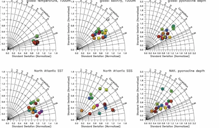
Taylor diagrams (Fig. 1) show that temperature is generally better constrained by the models than salin-ity, indicating some problems in the models represent-ing the hydrological cycle of the atmosphere. The pyc-nocline depth shows the weakest correlations, as errors
from T and S may sum up. All models perform best when global values over the entire depth of the water column are considered (not shown). However, this is not surprising since large areas, in particular the deep ocean, are still close to the initial conditions. The more the data subsets are confined to the surface ocean, the higher the model spread gets, as shown in the Taylor diagrams. According to the Taylor skill score, the CCCMA CGCM3.1-t63 and the Geophysical Fluid Dy-namics Laboratory Climate Model version 2.1 (GFDL CM2.1) yield the highest scores and thus the highest weights W (Fig. 2; Table 1). The three Goddard Insti-tute for Space Studies (GISS) models appear to be poor when assessed by global data distributions, but yield much higher weights when only assessed by North At-lantic upper ocean quantities. For the latter, the MIUB ECHO model turns out to be poorest but shows inter-mediate weights when assessed by global data distribu-tions.
Similar model skills and weights are obtained by the rms error assessment, which considers also systematic errors between the models and observations at every single grid point. Here, the GFDL CM2.1 clearly shows
FIG. 1. Taylor diagrams showing correlations and normalized std dev of the modeled vs observed (left) T, (middle) S, and (right) PD values for data from the (top) upper 1000 m of the water column and (bottom) North Atlantic surface water. The radial coordinates display the modeled vs observed correlation coefficients, while on the x axis the normalized std dev (modeled std dev divided by measured std dev) is plotted. A model perfectly matching the observations would reside in point (1, 1). Model numbers shown within the circles are according to the numbering in Table 1.
the best performance for all three data subsets, but the Met Office Hadley Centre model (UKMO HADLEY) also has a weight of almost 1 (Fig. 3). Again, the GISS models seem to perform rather poorly when assessed by global data but distinctly better when considering the North Atlantic. The Flexible Global Ocean–Atmo-sphere–Land System Model gridpoint version 1.0 (IAP FGOALS-g1.0) is a relatively poor simulation accord-ing to its North Atlantic T, S, and PD values but yields intermediate weights for global data distributions.
As a third and completely different approach, model performance is assessed by comparison with observa-tion-based mass transport estimates. The latter amount to 14–18 Sverdrups (sv; 1 Sv ⬅ 106 m3s⫺1) at 24°N (Ganachaud and Wunsch 2000; Lumpkin and Speer 2003), 13–19 Sv at 48°N (Ganachaud 2003), and 11.5– 22.9 Sv at the respective maximum (Smethie and Fine 2001; Talley et al. 2003). According to this assessment, five models perform very well, matching the ranges of all three estimates: the Model for Interdisciplinary Research on Climate, medium-resolution version [MIROC(medres)], MIUB ECHO, MRI CGCM2.3.2, the National Center for Atmospheric Research Com-munity Climate System Model version 3 (NCAR CCSM3.0), and UKMO HADLEY (Fig. 4). The GFDL CM2.1, which is the best according to T, S, and PD
evaluations, consistently has too high mass transports but still yields a weight higher than 0.8. Three models (IAP FGOALS and the two CCCMA models) are clearly inconsistent with the observations.
b. Evolution of the Atlantic MOC
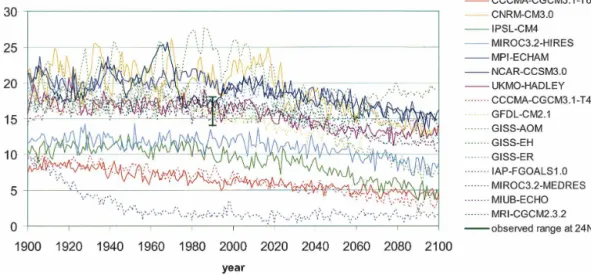
The Atlantic meridional overturning streamfunction is combined from model experiments 20C3M and SRESA1B where available to show the evolution dur-ing the twentieth and twenty-first centuries (Fig. 5). There is still considerable spread among the models simulating the present overturning (MOC) at 30°N, which is a similar result to that in the Third Assessment Report (TAR). The 1900 transports diverge by more than 10 Sv and there are large differences in interan-nual and interdecadal variability. About half of the models simulate overturning rates between 14 and 18 Sv for 1980–99, which is in the range of observation-based estimates (Ganachaud and Wunsch 2000; Lump-kin and Speer 2003). Except for one model (IAP FGOALS), where the MOC collapses already at the beginning, all models predict a gradual weakening of the MOC during the present century (2000–2100), but predicted changes in interannual and interdecadal variations as well as the amount of future reduction differ largely between individual models. Nevertheless,
FIG. 2. Weight factors according to the Taylor skill evaluation. Please note that in those cases where a single bar is missing, the respective model is assigned a weight of zero.
none of the models predicts a sudden drop and/or com-plete shutdown of the MOC over the twenty-first cen-tury.
The multimodel weighted mean estimates of the MOC show a reduction in the overturning from the year 2000 to 2100 by about 4 Sv, which corresponds to
a decline of about 25% (Fig. 6). The arithmetic (un-weighted) mean lies within the lower range of the dif-ferent weighted projections, also decreasing by about 4 Sv (⬃25%). There are some differences between the weighted MOC projections obtained by different weighting procedures (Fig. 6). Weighted estimates
cal-FIG. 4. Weight factors yielded by assessing model quality from comparing modeled MOC rates with observation-based mass transport estimates. Please note that the missing bar for IAP FGOALS-g1.0 means that this is the weakest model with a weight of zero. Furthermore, there are five models that fit into all three ranges of mass transport estimates, so that all five models yield the highest possible weight of one.
culated from the Taylor assessment, for instance, tend to put more weight on those models with weaker over-turning relative to those from the rms calculations. The weighted estimate based on the comparison with ob-served mass transports clearly emphasizes those models with intermediate–higher overturning rates, as they match the observed range of mass transports best.
The results depend also on the choice of data subsets used for skill calculations. Using North Atlantic T, S,
and PD for model assessment yields always higher-weighted overturning values for both Taylor and rms skill than the respective calculations based on global and global upper-1000-m data. Except for the weighted projection based on the Taylor skill for global data from the entire water column, all weighted projections yield present day MOC values in the range of observa-tion-based mass transport estimates (black bar in Fig. 6). The result of a generally decreasing MOC by about
FIG. 6. Weighted best estimates of the MOC projections according to the different skill/weight calculations performed. Even though there is some spread between the different best estimates, all of them show a reduction of the future MOC of about 25%, which is remarkably constant between the different approaches. Furthermore, except for the global Taylor model assessment, all weighted projections for present day fit within the range of observed mass transport estimates [i.e., by this means each of the individual methods (except Taylor global) seems to be justified].
FIG. 5. MOC rates at 30°N of all models used in the current study. There is considerable spread between
individual models, even in the year 1900, which is still close to initial conditions. Half of the models match observation-based mass transport estimates for present day (14–18 Sv), which is indicated by the black bar. Dashed lines indicate models where the average of two or more ensemble runs were used.
25% during the twenty-first century is remarkably in-sensitive to the method of model evaluation. The changes of individual model projections, at the same time, show large spread with MOC rates decreasing between 0.2 and 8.4 Sv, or 8%–54%, respectively (Table 1).
For most weighted MOC projections the weighted standard deviations are almost identical and match those from the arithmetic mean. However, those for the North Atlantic rms and the mass transport cases are considerably lower (Fig. 10), as in those cases the 3–4 models that perform best are lying very close to the finally achieved best estimate, so this result is rather trivial.
c. Global warming
The gradual decline of the MOC during the twenty-first century is associated with a weakening of the northward heat transport in the Atlantic Ocean. For example, at 30°N both show a strong positive
correla-tion for most of the available models (Fig. 7). The heat transport is predicted to decrease from 0.7 to 0.65 PW (arithmetic mean), that is, by 7% during the twenty-first century. Nevertheless, there is significant warming to be expected for Europe (35°–70°N, 10°W–30°E) with a weighted (and unweighted) mean increase of about 3 K until 2100 (Fig. 8). This temperature increase can be explained by a stronger horizontal gyre circulation in a warmer climate that largely compensates for the re-duced northward heat transport from a weaker MOC (Drijfhout and Hazeleger 2006). The amount of warm-ing over Europe is similar to the global warmwarm-ing mag-nitude (⫹2.7 K; not shown).
5. Discussion
Our analysis of a multimodel ensemble for the future development of the Atlantic MOC has shown that there is still a large spread between models concerning the strength of meridional overturning. However, the
mod-FIG. 7. Relation of MOC and northward heat transport showing that for most of the models there is a strong positive correlation between both parameters. Each point represents an annual average value for the period of 1850–2000.
els agree on a gradual decline of the MOC during the twenty-first century. None of the models predicts abrupt changes or a complete shutdown of the MOC. We have demonstrated that different ways to assess model performance yield different best estimates for future projections of the MOC. Therefore, as already mentioned in Schmittner et al. (2005), one needs to evaluate whether the chosen parameters (T, S, PD, and mass transport estimates) are suitable parameters to assess model performance in terms of MOC represen-tation and which skill calculation is the best. To address the first question we have performed a model to model comparison, using each model as a reference to test whether those models that have similar T and S distri-butions produce similar overturning rates. For data from the North Atlantic upper 1000 m, the correlation coefficient of the rms errors of T and S versus the de-viation from the referenced MOC is on average R ⫽ 0.55 with 13 out of 19 models being higher than 0.5. This indicates that T and S are suitable parameters to assess the MOC. A straightforward way to evaluate the qual-ity of our skill calculations is to compare the weights obtained from the Taylor and the rms skill calculations with those from the observation-based mass transport estimates, as these are two independent ways of model assessment. Consequently, a model that is good/bad in
the performance of T, S, and PD should also be good/ bad in the performance of mass transport and vice versa. This should especially hold for model assess-ments using data from the North Atlantic, as this is a key region determining the strength of the MOC. In our analysis, this agreement between different approaches is more or less the case, as shown by Fig. 9. Those models that perform well with respect to the mass transport estimates are also good in the assessment by the Taylor and rms skills. Similarly, the models with high weights according the Taylor and rms skills also yield high weights according the mass transport skill. The same applies to those models with intermediate and weaker performances (Fig. 9). In 9 out of 16 cases, the weight obtained by the Taylor skill is closer to the mass transport weight, while the rms weights are only in 6 cases closer. Nevertheless, the Taylor weights some-times show much larger deviations from the mass trans-port weights than the rms weights; particularly for the weakest model, IAP FGOALS, the Taylor skill indi-cates a relatively high weight, even though the MOC has collapsed. The skill calculations based on the mass transport estimates show some deficiency, as the range of mass transports is comparatively large and thus easy to match. In addition, the index for the maximum mass transport rate is a rather poor constraint, as it has a
FIG. 8. Projections of surface air temperatures over the European continent (35°–70°N, 10°W–30°E) for the future 100 yr (2000–2100) for individual models (black lines), as well as the arithmetic and weighted estimate (dashed line) based on weights obtained from the rms model assessment for data from the North Atlantic surface waters.
lower limit of 11.5 Sv, which is even below the lower limits of the other two estimates at 24°N (14 Sv) and 48°N (13 Sv). From this comparison of different skill calculations it can be concluded that none of the meth-ods is superior to another and that probably a combi-nation of different methods is the best way to assess model performance, confirming the approach used in Schmittner et al. (2005).
A further aspect that is of interest when regarding
future MOC projections is the influence of climate sen-sitivity. As different models exhibit different climate sensitivities, one might assume that those models with higher climate sensitivities may respond more strongly to the applied greenhouse forcing. However, we found that there is no correlation between climate sensitivity and MOC change (Fig. 11). This indicates that the re-spective MOC changes are robust and independent of model sensitivity. Furthermore, there is no correlation
FIG. 10. Std dev for the MOC developments of different weighted (or unweighted) projections. FIG. 9. Comparison of weight factors obtained for different methods by assessing model quality for data from
between Southern Ocean wind stress and overturning strength, as proposed by Kuhlbrodt et al. (2007).
The assessment of model performance could be im-proved by including more physical constraints of the MOC behavior. For example, small-scale processes like deep convection in the Labrador Sea and/or overflows across the Greenland–Iceland–Scotland Ridge should be taken into account if model resolution is adequate to represent those mechanisms. However, such measure-ments are relatively sparse. Another factor that is not taken into account in this model design is the effect of ice sheet melting, which was only included in the L’Institut Pierre-Simon Laplace Coupled Model ver-sion 4 (IPSL CM4) model here. Especially the melting of the Greenland ice sheet, which is predicted as a con-sequence of global warming, will lead to an additional freshwater input into the North Atlantic, which may lead to a further weakening of the MOC (Swingedouw et al. 2006). However, the amount of glacier melting during the twenty-first century is still under debate.
6. Conclusions
The assessment of model performance, as applied here to a multimodel ensemble, is proposed to improve the reliability of future climate projections, as
uncer-tainties from individual model simulations are effec-tively reduced. Temperature T, salinity S, pycnocline depth (PD), and observed mass transport estimates are suitable parameters to evaluate model performance. Skill calculations should be based on a combination of correlations (Taylor skill) and rms errors of T, S, and PD as well as observation-based mass transport esti-mates, as no method has turned out to be superior to the others and so different independent approaches are included. According to our findings, a decrease of the MOC over the last 40 yr as described by Bryden et al. (2005) is not seen in any of the models used here, but the future MOC is predicted to decline by about 25% during the twenty-first century. However, additional ef-fects of freshwater input from ice melt (e.g., Greenland) are not considered. The predicted future reduction of the MOC leads to a reduced northward heat transport in the Atlantic by about 7%. This is not sufficient to avoid greenhouse warming over Europe, which will warm during the twenty-first century by about 3 K on average based on these model results.
Acknowledgments. We thank Ronald Stouffer and
two anonymous reviewers for their very helpful and constructive comments, which helped to significantly improve the manuscript. This work was supported by
FIG. 11. Data of climate sensitivities of individual models (as far as available) displayed vs MOC change with absolute values in Sv (black dots; left scale) and relative changes in percent (gray dots; right scale), showing that there is no relation between climate sensitivity in the models and the amount of MOC change.
the German CLIVAR and European ENSEMBLES projects and the SFB 460. We acknowledge the inter-national modeling groups for providing their data for analysis, the Program for Climate Model Diagnosis and Intercomparison (PCMDI) for collecting and archiving the model data, the JSC/CLIVAR Working Group on coupled Modeling (WGCM) and their Coupled Model Intercomparison Project (CMIP) and Climate Simula-tion Panel for organizing the model data analysis activ-ity, and the IPCC WG1 TSU for technical support. The IPCC Data Archive at Lawrence Livermore National Laboratory is supported by the Office of Science, U.S. Department of Energy.
REFERENCES
Bryden, H. L., H. R. Longworth, and S. A. Cunningham, 2005: Slowing of the Atlantic meridional overturning circulation at 25°N. Nature, 438, 655–657.
Conkright, M. E., R. A. Locarnini, H. E. Garcia, T. D. O’Brien, T. P. Boyer, C. Stephens, and J. I. Antonov, 2002: World Ocean Atlas 2001: Objective analyses, data statistics, and fig-ures CD-ROM documentation, NOAA Internal Rep. 17, 17 pp.
Drijfhout, S. S., and W. Hazeleger, 2006: Changes in MOC and gyre-induced Atlantic Ocean heat transport. Geophys. Res. Lett., 33, L07707, doi:10.1029/2006GL025807.
Fraedrich, K., and K. M. Leslie, 1987: Combining predictive schemes in short-term forecasting. Mon. Wea. Rev., 115, 1640–1644.
——, and N. R. Smith, 1989: Combining predictive schemes in long-range forecasting. J. Climate, 2, 291–294.
Ganachaud, A., 2003: Large-scale mass transports, water mass formation, and diffusivities estimated from World Ocean Cir-culation Experiment (WOCE) hydrographic data. J. Geo-phys. Res., 108, 3213, doi:10.1029/2002JC001565.
——, and C. Wunsch, 2000: Improved estimates of global ocean circulation, heat transport and mixing from hydrographic data. Nature, 408, 453–457.
Gnanadesikan, A., R. D. Slater, N. Gruber, and J. L. Sarmiento, 2002: Oceanic vertical exchange and new production: A com-parison between models and observations. Deep-Sea Res. II,
49, 363–401.
Gregory, J. M., and Coauthors, 2005: A model intercomparison of changes in the Atlantic thermohaline circulation in response to increasing atmospheric CO2concentration. Geophys. Res. Lett., 32, L12703, doi:10.1029/2005GL023209.
Houghton, J. T., Y. Ding, D. J. Griggs, M. Noguer, P. J. van der Linden, X. Dai, K. Maskell, and C. A. Johnson, Eds., 2001: Climate Change 2001: The Scientific Basis. Cambridge Uni-versity Press, 881 pp.
Knutti, R., T. F. Stocker, F. Joos, and G. K. Plattner, 2003: Proba-bilistic climate change projections using neural networks. Cli-mate Dyn., 21, 257–272.
Kuhlbrodt, T., A. Griesel, M. Montoya, A. Levermann, M. Hoff-mann, and S. Rahmstorf, 2007: On the driving processes of the Atlantic Meridional Overturning Circulation. Rev. Geo-phys., in press.
Lumpkin, R., and K. Speer, 2003: Large-scale vertical and hori-zontal circulation in the North Atlantic Ocean. J. Phys. Oceanogr., 33, 1902–1920.
Manabe, S., 1993: Century-scale effects of increased atmospheric CO2on the ocean-atmosphere system. Nature, 364, 215–218. ——, and R. J. Stouffer, 1988: Two stable equilibria of a coupled
ocean–atmosphere model. J. Climate, 1, 841–866.
Metzger, S., M. Latif, and K. Fraedrich, 2004: Combining ENSO forecasts: A feasibility study. Mon. Wea. Rev., 132, 456–472. Murphy, J. M., D. M. H. Sexton, D. N. Barnett, G. S. Jones, M. J. Webb, M. Collins, and D. A. Stainforth, 2004: Quantification of modelling uncertainties in a large ensemble of climate change simulations. Nature, 430, 768–772.
Palmer, T. N., and Coauthors, 2004: Development of a European Multimodel Ensemble System for Seasonal-to-Interannual Prediction (DEMETER). Bull. Amer. Meteor. Soc., 85, 853– 872.
Rahmstorf, S., 2003: Thermohaline circulation: The current cli-mate. Nature, 421, 699.
Schmittner, A., M. Latif, and B. Schneider, 2005: Model projec-tions of the North Atlantic thermohaline circulation for the twenty-first century assessed by observations. Geophys. Res. Lett., 32, L23710, doi:10.1029/2005GL024368.
Smethie, W. M., and R. A. Fine, 2001: Rates of North Atlantic deep water formation calculated from chlorofluorocarbon in-ventories. Deep-Sea Res. I, 48, 189–215.
Stocker, T. F, and A. Schmittner, 1997: Influence of CO2emission rates on the stability of the thermohaline circulation. Nature,
388, 862–865.
Stouffer, R. J., and Coauthors, 2006: Investigating the causes of the response of the thermohaline circulation to past and fu-ture climate changes. J. Climate, 19, 1365–1387.
Swingedouw, D., P. Braconnot, and O. Marti, 2006: Sensitivity of the Atlantic Meridional Overturning Circulation to the melt-ing from northern glaciers in climate change experiments. Geophys. Res. Lett., 33, L07711, doi:10.1029/2006GL025765. Talley, L. D., J. L. Reid, and P. E. Robbins, 2003: Data-based meridional overturning streamfunctions for the global ocean. J. Climate, 16, 3213–3226.
Taylor, K. E., 2001: Summarizing multiple aspects of model per-formance in a single diagram. J. Geophys. Res., 106, 7183– 7192.
Trenberth, K. E., and J. M. Caron, 2001: Estimates of meridional atmosphere and ocean heat transports. J. Climate, 14, 3433– 3443.