Implementation of position assimilation for ARGO floats in a realistic Mediterranean Sea OPA model and twin experiment testing

(1)

HAL Id: hal-00298378

https://hal.archives-ouvertes.fr/hal-00298378

Submitted on 18 May 2006

HAL is a multi-disciplinary open access

archive for the deposit and dissemination of sci-entific research documents, whether they are pub-lished or not. The documents may come from teaching and research institutions in France or abroad, or from public or private research centers.

L’archive ouverte pluridisciplinaire HAL, est destinée au dépôt et à la diffusion de documents scientifiques de niveau recherche, publiés ou non, émanant des établissements d’enseignement et de recherche français ou étrangers, des laboratoires publics ou privés.

Implementation of position assimilation for ARGO floats

in a realistic Mediterranean Sea OPA model and twin

experiment testing

V. Taillandier, A. Griffa

To cite this version:

V. Taillandier, A. Griffa. Implementation of position assimilation for ARGO floats in a realistic Mediterranean Sea OPA model and twin experiment testing. Ocean Science Discussions, European Geosciences Union, 2006, 3 (3), pp.255-289. �hal-00298378�

(2)

OSD

3, 255–289, 2006

Implementation of ARGO position

assimilation V. Taillandier and A. Griffa

Title Page Abstract Introduction Conclusions References Tables Figures J I J I Back Close

Full Screen / Esc

Printer-friendly Version Interactive Discussion

EGU Ocean Sci. Discuss., 3, 255–289, 2006

www.ocean-sci-discuss.net/3/255/2006/ © Author(s) 2006. This work is licensed under a Creative Commons License.

Ocean Science Discussions

Papers published in Ocean Science Discussions are under open-access review for the journal Ocean Science

Implementation of position assimilation

for ARGO floats in a realistic

Mediterranean Sea OPA model and twin

experiment testing

V. Taillandier1and A. Griffa1,2

1

CNR-ISMAR, Forte Santa Teresa, 19036 Lerici, La Spezia, Italy

2

RSMAS, University of Miami, 4600 Rickenbacker Causeway, Miami, FL, USA Received: 23 February 2006 – Accepted: 9 April 2006 – Published: 18 May 2006 Correspondence to: V. Taillandier ([email protected])

(3)

OSD

3, 255–289, 2006

Full Screen / Esc

EGU

Abstract

In this paper, a Lagrangian assimilation method is presented and implemented in a realistic OPA OGCM with the goal of providing an assessment of the assimilation of realistic Argo float position data. We focus on an application in the Mediterranean Sea, where in the framework of the MFSTEP project an array of Argo floats have

5

been deployed with parking depth at 350 m and sampling interval of 5 days. In order to quantitatively test the method, the “twin experiment” approach is followed and synthetic trajectories are considered. The method is first tested using “perfect” data, i.e. without shear drift errors and with relatively high coverage. Results show that the assimilation is effective, correcting the velocity field at the parking depth, as well as the velocity

10

profiles and the geostrophically adjusted mass field. We then consider the impact of realistic datasets, which are spatially sparse and characterized by shear drift errors. Such data provide a limited global correction of the model state, but they efficiently act on the location, intensity and shape of the described mesoscale structures of the intermediate circulation.

15

1 Introduction

Lagrangian measurements have experienced a dramatic increase in recent years. The Argo program, consisting of a broad-scale global array of floats, is now one of the main components of the ocean observing system (http://www.argo.ucsd.edu). Argo floats are autonomous profiling floats that spend most of their life freely drifting at a

20

given parking depth, and that surface at a regular time interval measuring temperature and salinity (TS) while ascending through the water column. When at the surface, they communicate information on position and TS profiles via satellite. Position data provide information on the ocean current at the parking depth, while TS data characterize the water masses.

25

(4)

OSD

3, 255–289, 2006

Full Screen / Esc

EGU be used in operational systems for assimilation in Ocean General Circulation Models

(OGCM’s). Data on TS profiles are presently routinely assimilated in many operational systems (http://www.argo.ucsd.edu/FrUse by Operational.html) while position data are not included yet. On the other hand, float positions r contain information on an

im-portant model state variable, the Eulerian velocityu. The relationship between r and

5

u is highly nonlinear, d r/d t=u(r, t), therefore the assimilation of r poses significant

challenges. The first theoretical works on position assimilation (Ishikawa et al., 1996) simply circumvented this problem using the quantity ∆r/∆t, where ∆t is the interval between successive position information, as a proxy foru. This approximation holds

for very small∆t with respect to the typical Lagrangian time scale T_L(Molcard et al.,

10

2003), which is of the order of 1–3 days at the surface and 5–10 days in the subsurface. In the case of Argo floats, since∆t and T_L are approximately of the same order, the approximation is clearly violated and appropriate assimilation methods that take into account the true nature of the observations have to be considered.

In the last few years, growing attention has been given and various

methodolo-15

gies proposed to assimilate position data. Different Lagrangian approaches have been investigated, going from Optimal Interpolation (OI) (Molcard et al., 2003, 2005;

¨

Ozg ¨okmen et al., 2003), Kalman filtering (Ide et al., 2002; Kuznetsov et al., 2003), to variational techniques (Kamachi and O’ Brien, 1995; Nodet, 2006; Taillandier et al., 2006a). They have been tested mostly using simplified dynamical systems, such

20

as point vortices (Ide et al., 2002), or academic model configurations (Kamachi and O’Brien, 1995; Molcard et al., 2005). Even though the results are very encouraging and show the high potential of assimilating Lagrangian data, there are still a number of issues to be addressed regarding the actual application to Argo data assimilation in operational OGCM.

25

The first challenge to be addressed is the implementation of these assimilation meth-ods in realistic circulation models. In particular, with respect to previous applications in idealized model configurations with a reduced number of isopycnal layers (Molcard et al., 2005), expected improvements should include complex geometry and topography,

(5)

OSD

3, 255–289, 2006

Full Screen / Esc

EGU continuous stratification and TS mass variables in the model state. Other challenges

are inherent to the nature and distribution of the Argo datasets. NRT position infor-mation are obtained when the floats reach the ocean surface and communicate via satellite. Such surface position data provide information on the subsurface drift (at the parking depth) contaminated by “shear errors” due to additional drifts experienced

dur-5

ing ascent and descent motions (Park et al., 2005). The impact of such errors needs to be evaluated and possible techniques to account for it should be investigated. Also, Argo float positions are provided at intervals∆t of the order (or even greater) than T_L, so that successiver along observed trajectories might be weakly correlated. Therefore

the information content in terms of velocity might be degraded (Molcard et al., 2003).

10

Finally, the realistic coverage of Argo floats in a given region of the world ocean is expected to be quite low to resolve the mesoscale features of the circulation. These different aspects have to be tested in order to verify the impact and potential of Argo position data if included in operational observing systems.

In this paper we present a Lagrangian assimilation method for realistic OGCM’s. The

15

various points indicated above are tested with the goal of providing a complete assess-ment of the assimilation of realistic Argo floats. The inverse method builds on previous works (Molcard et al., 2003, 2005; Taillandier et al., 2006a) and conceptually follows the same three main steps as in Molcard et al. (2005). First the position datar are

used to correct the velocity fieldu at the parking depth z_pusing the variational method

20

developed in Taillandier et al. (2006a). Then the velocity correction is projected over the water column using statistical correlations while maintaining mass conservation. And finally the TS mass field is corrected in geostrophic balance with the correctedu

profiles using a variational approach (Talangrand and Courtier, 1987), based on the thermal wind and on the equation of state.

25

Here we consider a specific application to a realistic OPA model of the Mediterranean Sea. In the framework of the MFSTEP project (Pinardi et al., 2003;http://www.bo.ingv. it/mfstep/), a component of the world wide Argo project has been carried out in the Mediterranean Sea. A total of more than 20 floats have been deployed in the basin,

(6)

OSD

3, 255–289, 2006

Full Screen / Esc

EGU characterized by a time interval∆t of approximately 5 days and by a parking depth z_p

of 350 m (Poulain, 2005). In order to test the performances of the assimilation method in the “twin experiment” approach, synthetic floats with characteristics similar to the in-situ ones are released in a numerical circulation to be identified. The sensitivity of the Lagrangian analysis to shear errors and low coverage is considered in a second

5

time.

The paper is organized as follows. The method is presented in Sect. 2, while the set up for the numerical experiments is given in Sect. 3. The experiment results are presented in Sect. 4. Assimilation skills with realistic Argo type data are investigated in Sect. 5. Summary and discussion are provided in Sect. 6.

10

2 Methodological aspects

The analysed (estimated) circulation is obtained from float position information by cor-recting a prior (background) circulation in a sequential way. Such model state correc-tion is provided every ∆t=5 days according to the cycling design of the Argo floats. Estimations of the velocity fieldu and of the corresponding mass field (T , S) are

de-15

tailed in the following Sects. 2.1 and 2.2, respectively, for each 5 day sequence, while the practical implementation of the method is summarized in Sect. 2.3.

2.1 Estimation of the model velocity field

The velocity field at the parking depth z_p is estimated from Argo data using the vari-ational method developed by Taillandier et al. (2006a). The method provides a

bi-20

dimensional velocity increment ∆u(z_p) for each 5 day sequence separating two suc-cessive Argo float positions. In this approach, u(z_p) is estimated minimizing a cost function which measures the distance between the observed float position at the end of the sequence and the position of a prior trajectory advected in the background ve-locity field.∆u(z_p) is therefore a time-independent correction (for the given sequence)

(7)

OSD

3, 255–289, 2006

Full Screen / Esc

EGU ofu(z_p) along the prior trajectory. Note that shear drifts occurring on vertical float

mo-tions can be taken into account in the computation of the prior trajectory but onlyu(z_p) is estimated.

This variational method has been tested in Taillandier et al. (2006a), considering its performance by varying number of floats P and time sampling ∆t. The results are

5

positive, showing that the approach is effective and robust. Moreover, the method pro-vides significant advantages with respect to the previous works of Molcard et al. (2003, 2005), since it expands the velocity correction all along trajectories and uses an appro-priate covariance matrix. We notice that in Taillandier et al. (2006a) an important issue was discussed for the case of∆t of the order or bigger than T_L. This is of potential

inter-10

est here given that T_Lis expected to be approximately of the same order as∆t=5 days. It is pointed out that when strong vortices are sampled by various floats, it can happen that successive positions “cross” each other because the vortex curvature is not re-solved by the trajectory sampling. Such coherent structures are therefore not correctly estimated, since the obtained flow converges toward the crossing points. This

prob-15

lem, which is inherent to the data, was illustrated in the case where the velocity field is reconstructed using data only, i.e. without prior circulation. In the experiments con-sidered here, we expect that the use of prior model circulations, and consequently the use of additional information on the curvature, will help preventing this phenomenon. We will come back on this issue discussing the numerical results in Sect. 4.

20

In first approximation for regional and oceanic circulation scales, horizontal and ver-tical correlations of the motion can be separated using linear regression profiles (Os-chlies and Willebrand, 1996). Note that horizontal velocity correlations are specified by the length of mesoscale structures described by the float trajectories (Taillandier et al., 2006a). As discussed in Molcard et al. (2005), the velocity increment∆u(z_p) obtained

25

from float positions at z_pcan be projected on the water column as

∆u(z) = R(z).∆u(zp), z ∈ [0, h] (1)

where h is the depth of the basin and R represents the vertical projection operator. R(z) is computed from seasonal and spatial averages (in quasi-homogeneous regions)

(8)

OSD

3, 255–289, 2006

Full Screen / Esc

EGU of the linear regression coefficients linking each velocity component at depth z with

velocity at z_p.

This projection of ∆u(z_p) is funded on statistical means, without any constraint on model consistency. In order to introduce some dynamical constraints, we do enforce the assumption of basin volume conservation, in agreement with the continuity

equa-5

tion. In a rigid lid formulation, the barotropic flow increment can be expressed from Eq. (1) as

∆U = ∆u(zp). ∫

[0,h]

R(z).d z (2)

∆U is further imposed to be non divergent and re-computed from the diagnostic stream function. After that, the updated barotropic flow increment∆U, now in model

consis-10

tency, is used to redefine the velocity increment as ∆u(z) = R(z).[ ∫

[0,h]

R(z).d z]−1.∆U, z ∈ [0, h] (3)

This normalisation to the flat bottom case allows to smooth horizontal discrepancies on shallow zones, specially along the land-sea interface at the parking depth.

2.2 Estimation of a dynamically consistent mass field

15

For mesoscale open sea applications like the present one, the isopycnal slopes can be adjusted, at least in first approximation, to the velocity increment∆u (expressed in Eq. 3) in agreement with the thermal wind equation (Oschlies and Willebrand, 1996). So the mass field estimation is provided by the resolution of a static inverse problem formulated in the following variational approach.

20

Considering a prior model state (u, T , S), a variation δu of the velocity field infers

a variation of its vertical shear δσ=∂_zδu. This vertical structure is maintained by a

density variation δρ in geostrophic equilibrium as

(9)

OSD

3, 255–289, 2006

Full Screen / Esc

EGU where g is the gravity, ρ_o the density of reference, f the Coriolis parameter,k the

up-ward unit vector and ∇ the horizontal gradient. The density variation δρ is linearly expressed with respect to the equation of state. In case of a best-fit polynomial for-mulation (e.g. the one of Jackett and McDougall, 1995), the first order perturbation of density around its prior value ρ= P_{i ,j}α_{i j}.Ti.Sj is taken from the linear equation of state

5

δρ=X

i ,j

α_{i j}.Ti−1.Sj−1.(i .S.δT + j.T.δS) (5)

where δT and δS are the respective variations on the prior temperature and salinity profiles.

Here, we require that the shear variation∆σ=∂_z∆u provided by the analysis of the float positions (Eq. 3) is fitted to the geostrophic velocity shear variation defined by

10

Eq. (4). This latter can be expressed using Eqs. (4–5) by δσ=M.(δT , δS), where M is linear operator. The inverse problem consists in finding the best combination (δT , δS) that minimises the cost function

J= (∆σ − M.(δT, δS))T.(∆σ − M.(δT, δS)) (6)

whereT is the vector transpose. In numerical practice, J is minimised using the

steep-15

est descent algorithm M1QN3 (Gilbert and Lemar ´echal, 1989), in the direction of the gradient

∇J _{= −B.M}T_.(_{∆σ − M.(δT, δS))} ₍₇₎

where the linear operatorMT is governed by the adjoint equations of Eqs. (4–5), andB

is classically defined by background error covariances. For the construction ofB,

cross-20

covariances between temperature and salinity are not considered as the balance on these two variables is explicitly constrained by the equation of state (Eq. 5). So only the univariate components are required and described by the field variance. In numerical practice, seasonal and space averages of the standard deviation profiles for TS define the diagonal matrixB.

(10)

OSD

3, 255–289, 2006

Full Screen / Esc

EGU 2.3 Assimilation procedures

The assimilation procedure has been implemented in two different ways, referred to as “state of the art” and “operational” respectively. Both procedures have been tested in the twin experiments presented in the following.

In the procedure “state of art”, variations of Argo float positions during each

cy-5

cle/sequence are used to estimate the velocity and mass fields at the initial time of the assimilation sequence. The model is then run forward again for the considered se-quence using the corrected initial conditions, so that prior model state and trajectories are updated with respect to the initial state estimate. This procedure is characterised by a high computational cost as the CPU time of a forward model run is doubled, in

10

addition to the estimation of the velocity and mass corrections. Note that CPU time requirements for a model state analysis is very small compared to a forward run.

In the procedure “operational”, variations of float positions during each cy-cle/sequence are used to estimate the velocity and mass fields at the final time of the assimilation sequence. Prior model state computed on the sequence determines

15

the model update on the next sequence, and the prior float trajectories are not up-dated. This procedure is characterised by an equivalent computational cost as for a single forward run, always in addition to velocity and mass estimation.

3 Experimental set up

3.1 Modelling the Mediterranean circulation

20

The numerical model used here is an extended version of the primitive equation model OPA with rigid lid (Madec et al., 1998), configured in the Mediterranean Sea. For the development and testing of the assimilation procedure, which is computationally de-manding, a horizontal resolution at 1/8 degree has been considered, while the statisti-cal prior information onR and B have been computed using a more refined resolution at

(11)

OSD

3, 255–289, 2006

Full Screen / Esc

EGU 1/16 degree. For both configurations a vertical discretization with 43 geopotential levels

is considered. The model is initialised from rest by climatological hydrological condi-tions from MEDATLAS. It is forced by daily winds and heat fluxes from the ECMWF atmospheric forcing fields during the period 1987–2004. The spin-up has been per-formed repeating the cycle three times. Characteristics of the general circulation and

5

of the transports at several straits are in good agreement with recent estimates from in-situ observations (B ´eranger et al., 2005).

We concentrate on a case study in the North Western Mediterranean Sea, during the winter season. This region has been chosen since it is a complex and interesting area with a vigorous mesoscale field even at 350 m. Moreover, a good coverage of

10

in-situ Argo floats has been maintained in this region during the MFSTEP project (http: //poseidon.ogs.trieste.it/WP4/product.html). As a first step, the statistical quantities have been computed from model outputs during 2000–2004. Horizontal motion scales, already described in Taillandier et al. (2006a) are characterized by typical mesoscale length scales of the order of 20–30 km, and associated Eulerian time scales of the order

15

of 20–30 days. Vertical correlations are computed from the velocity fields to defineR

(Eq. 1), and from the active tracer fields TS to define B (Eq. 7). These correlations

are computed independently for each velocity or tracer component, and averaged over the north western basin, to get winter mean representative profiles. As underlined in Sect. 2.2, only the variance profiles for tracer fields are involved in the construction

20

ofB. In the region of interest, maximum variance for temperature reaches 0.50◦C in the first 100 m, followed by a quick decrease to 0.15◦C in the intermediate layer. For salinity, the decrease from the maximum value of 0.12 PSU at surface is quasi linear, to reach 0.05 PSU at the parking depth.

Regression and correlation profiles for velocity are represented in Fig. 1. They are

25

very similar for the zonal and meridional components. The velocity variations on a large intermediate layer [150 m, 750 m] appear well correlated with velocity variations at the parking depth. Instead in the surface layer and in the deep layer, correlation values drop under 0.8. The linear regression coefficients decrease from 2.5 at sea surface

(12)

OSD

3, 255–289, 2006

Full Screen / Esc

EGU until 0.4 at sea bottom. The profile can be described by four straight lines: a surface

segment [0 m, 200 m] associated to a sharp slope, an intermediate segment [200 m, 600 m], a deep segment [600 m, 1000 m] associated to a slight slope, and a bottom segment after 1000 m without slope. Considering Eq. (1), the first order derivative of the regression profile is related to the relative intensity of the vertical shear variations.

5

As a consequence, the correction of the baroclinic velocity (Sect. 2.2) will be limited to the first 1000 m, and it is expected to be characterized by decreasing amplitude from the sea surface, as in three distinct layers quite well correlated.

3.2 Numerical experiments

The sensitivity and robustness of the assimilating system has been tested with a total

10

of seventeen simulation experiments. A first set of experiments (Sect. 4) is directly finalized at testing the methodology and the two different implementations of Sect. 2.3. It considers “ideal” data, i.e. data with no shear errors and with significant spatial cov-erage. Instead, a second set of experiments (Sect. 5) is finalized at investigating the method performance in “realistic” conditions for Argo float applications, i.e. in presence

15

of significant shear error and with reduced coverage.

The numerical protocol of experimentation follows the classical twin experiment ap-proach, and can be summarized as follows. Three different simulations are performed for each experiment using the circulation model (Sect. 3.1), all with the same forcing functions corresponding to the month of March 1999. The first run is correctly initialized

20

from the model state corresponding to 1 March 1999, and it represents the “truth” circu-lationutru. Synthetic floats are launched in the truth run and advected by the numerical velocity field. The second run is initialized from a “wrong” initial condition, correspond-ing to 1 March 2000, to represent our incomplete knowledge of the true state of the ocean. The position data extracted from the truth circulation are assimilated in this

25

run, providing the “estimated” fielduest. Finally, the third run provides a “background” circulationubck initialized with the same wrong initial condition as the assimilation run, but without data assimilation. It provides a reference simulation, where the wrong initial

(13)

OSD

3, 255–289, 2006

Full Screen / Esc

EGU conditions evolve according to forcing and dynamics. The success of the assimilation

is quantified in terms of convergence ofuest towardutru. In other words a successful assimilation is expected to correct the wrong initial conditions, driving the ocean state toward the truth.

The numerical trajectories are computed following the same cycle as in-situ Argo

5

floats, using a fourth order Runge-Kutta scheme for advection. The cumulated duration of vertical motion is fixed to half a day, while the residence time in subsurface is equal to 4.5 days. In our numerical experiments two sets of data have been extracted from the numerical trajectories: the “perfect data”, containing initial and final positions of each subsurface drift, that are utilized in the idealized experiments (Sect. 4), and the surface

10

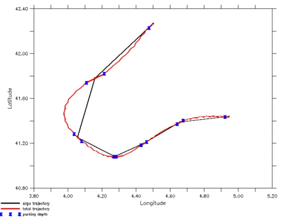
data, that take into account the shear drift and that are used in the realistic experiments (Sect. 5). For in-situ floats, only surface positions are available, provided in near-real time via satellite. In Fig. 2, an example of the difference between the “perfect” data (marked by crosses) and “realistic” data observed at the surface is shown along a single numerical trajectory.

15

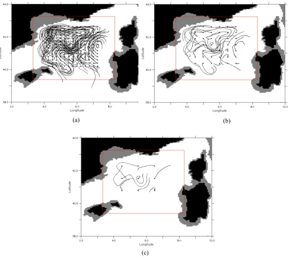
A total of 182 simulated Argo floats have been homogeneously released and ad-vected in the truth circulation during six cylces (Fig. 3). In the assimilation experiments, the influence of data coverage is studied varying the number of Argo type trajectories

P=182, 42, 9, 4, 3 extracted from the original set. In order to minimise the effects of

initial conditions (e.g. Toner et al., 2001; Molcard et al., 2006), in all cases the

homo-20

geneous release is maintained. As shown in Fig. 3, the Lagrangian description of the circulation shows an intense boundary current (the so-called Northern Current) charac-terized by meanders and recirculation cells. Given the long Eulerian time scale (20–30 days), the trajectories are indicative of mesoscale structures, but they quickly tend to get sparse when P decreases.

25

The assimilation system is quantitatively assessed using a measure of the adjust-ment ofuesttoutru. It is expressed by the non dimensional quantity

E (z, t)= ||utru(z, t) −uest(z, t)||2/||utru_{(z, t) −}_ubck_{(z, t)||}2 ₍₈₎ where ||u||2=uT.u. The normalization term in denominator is used to reduce the

(14)

de-OSD

3, 255–289, 2006

Full Screen / Esc

EGU pendency of the results from the specific realization, i.e. from the time evolution of

the background simulation. This measure is integrated over the computational region shown in Fig. 3. It can be applied at a given depth z or at a given sequence t.

4 Results of experiments with ideal data

The methodology (Sect. 2) is tested using perfect data (i.e. without shear error) and

5

considering the effects of decreasing coverage in a range of relatively high number of floats P=182, 42, 9. The two different procedures discussed in Sect. 2.3 are compared. The results are assessed first in terms of velocity estimation at the parking depth and then in terms of velocity and mass estimation over the whole water column.

4.1 Velocity estimation at the parking depth

10

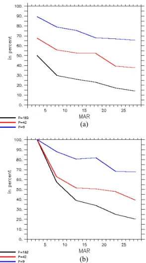
The first assessment focuses on the analysis of the circulation at the parking depth z_p. Results for P=182, 42, 9 are shown in Fig. 4 in terms of time evolution of the adjustment error E (t) (defined in Eq. 8) during the one month assimilation period using the two pro-cedures. For both of them, the adjustment of the velocity field at 350 m is increasingly better with data coverage, as expected. The mean slope of the error decrease varies

15

from 20% with low coverage (P=9) to 35% with high coverage (P =182). When consid-ering the sequence by sequence evolution of E (t), it appears that the major adjustment occurs during the first two analyses. After that, E (t) continues to decrease in average, but oscillations can occur especially for P=42 and P =9, with slight increases followed by marked decreases. This can be explained considering the following points of view.

20

In a fix point approximation (in which information locations do not change), the time scale characterising the assimilation adjustment is expected to coincide with the time scales of the circulation structures, i.e. with the time over which the information is cor-related. With high coverage (P=182), the fix point approximation can be assumed, and the obtained adjustment appears characterised by a constant decrease at the

(15)

OSD

3, 255–289, 2006

Full Screen / Esc

EGU rian time scale (∼20 days). With low coverage instead, and given the relatively long

Eulerian time scales, the velocity field can be assumed time-independent with respect to the scale of motion of the floats. In this frozen field approximation, local and fast adjustments to the truth circulation are provided at the information location and at the Lagangian time scale (order of 3–5 days). Successive adjustments are expected to

5

occur when the floats enter and sample new circulation structures, providing new in-formation. This appear to be the case for P=9 or P =42, where the decrease of E(t) is characterised by secondary gaps due to the renewal of data information.

A comparison of the two assimilation procedures can now be performed. In the pro-cedure “operational” (Fig. 4b), the effect of the model state correction for sequence (n)

10

appears at sequence (n+1). So this procedure only benefits of five analyses during the assimilation period, instead of six as for the procedure “state of art” (Fig. 4a). In terms of adjustment, the evolution of E (t) appears similar in both procedures but translated of one sequence. So the adjustments obtained at the final time with the procedure “operational”, E=70% for P =9, E=40% for P =42, 20% for P =182, are approximately

15

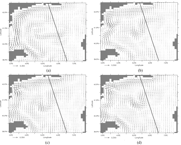
the same as the ones obtained a sequence before with the procedure “state of art”. An example of qualitative comparison between estimated and truth circulations at the parking depth is drawn for the representative data coverage of P=42 in Fig. 5. The results are similar for the two procedures, even though slight differences still remain on intensity and shape between the two estimated circulations. In both cases the

20

assimilation appears to efficiently correct the field, and the estimates tend to converge toward the truth field. The Northern Current confined along the coast in the background circulation appears wider in the estimated circulations. Its meandering and recirculating features present in the truth circulation appear well estimated. Both intense and weak mesoscale structures are replaced from their background location with respect to the

25

truth circulation.

We notice that in all the performed experiments, there is no evidence of problems in the velocity estimation when ∆t≥T_L as discussed in Taillandier et al. (2006a) (and mentioned in Sect. 2.1) did not emerge. No unrealistic convergence in the estimated

(16)

OSD

3, 255–289, 2006

Full Screen / Esc

EGU velocity field has been found. This might be partially due to the fact that the case in

Taillandier et al. (2006a) was extreme in terms of intense sampling of the core of a very energetic vortex, even though also in the present experiments strong recirculations and vortices are present and sampled at various rates, as shown in Fig. 3. More conceptually, we think that the main reason for the difference is that in Taillandier et

5

al. (2006a), the velocity field was reconstructed based on the float data only, while in the present experiments the data are assimilated in a model. The model provides a priori information on the velocity structure, so that the information on the curvature can be corrected avoiding the emergence of unrealistic velocity convergence and a correct estimate can be obtained.

10

4.2 Velocity estimation on the water column and impact of TS correction

The effect of the velocity estimation at the parking depth is now investigated on the other layers. The quality of the model state analyses from float positions depends on the velocity adjustment at depth, which is given directly by the shape of linear re-gression profiles (see Eq. 1) and indirectly by the mass field adjustment. This latter

15

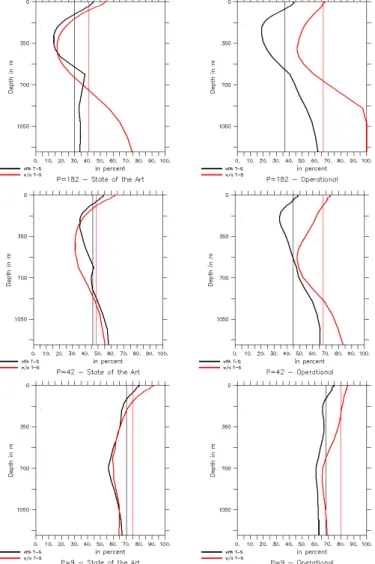
mechanism can either be forced through the estimation of temperature and salinity (Sect. 2.2), or lead by a passive relaxation of the mass field onto the estimated velocity field. In order to evaluate the impact of TS estimation, both approaches are tested when assimilating the three data sets P=182, 42, 9. The corresponding adjustment errors E (z) (given in Eq. 8 at the end of the assimilation period) are represented in

20

Fig. 6. It appears that the profiles E (z) are improved when obtained with TS estima-tion. This is particularly the case when the procedure “operational” is used. On the other hand, there is only a slight improvement when the procedure “state of art” is used. So the relaxation of the mass field is effectively operated during the sequence reanalysis, i.e. while it is set to the velocity estimate on the same sequence (Sect. 2.3).

25

These adjustment errors appear to decrease from the sea surface to a minimum value close to the parking depth, increasing then with depth. This is particularly accen-tuated with high data coverage (P=182), while the adjustments tend to be

(17)

homoge-OSD

3, 255–289, 2006

Full Screen / Esc

EGU neous on the water column with low data coverage (P=9). This general feature can be

explained considering the velocity correlations (Fig. 1) implicated in the vertical velocity projection (Eq. 1). As described in Sect. 3.1, the amplitudes of the velocity variations at the sea surface are at least twice than those in the intermediate layer, while sur-face and intermediate currents are weakly correlated. So adjustment errors obviously

5

increase in the surface layer. On the other hand, E (z) values on the deep layer are mainly governed by the barotropic flow adjustment in which the baroclinic structure of the model state analyses is involved. So the quality of velocity estimates in the deep layer is degraded because of the estimation of the baroclinic structure, through the specification of vertical velocity shear, which is poor at depth (Sect. 3.1). Moreover,

10

this degradation of E (z) in the deep layers is accentuated when the adjustment of the model mass field is not effective. As shown for the “operational” procedure (Fig. 6 left panels), adjustment errors of deep currents are increased in absence of mass field estimation.

A quantitative comparison of the effectiveness of the two assimilation procedures

15

versus z can be performed comparing the results in the left and right panels of Fig. 6. As it can be seen, results at the parking depth (discussed in Sect. 4.1) appear to hold also for an extended layer [150 m, 500 m]. For both procedures, the adjustment errors increase at the sea surface and in the deep layer. With low data coverage, this growth is limited and the results of the two procedures are similar. On the other hand, when

20

the coverage is high (P=182, 42), the growth of E(z) at depth is limited (∼20%) with the “state of art” procedure while is higher in the “operational” procedure (∼35%). Notice that adjustments of vertical mean currents are of same order for both procedures.

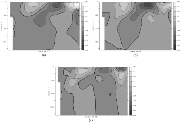
In order to better visualize the TS correction, a hydrologic section is extracted along the NW-SE transect shown in Fig. 5. The background, truth and estimated mass fields

25

given at the end of the assimilation period are presented in Fig. 7 for the case of

P=42. Note that estimates of the mass field and of the horizontal velocity (Fig. 5) are

obtained from the same data set. Then each mesoscale structure crossed by the sec-tion appears geostrophically maintained in the intermediate layer by the isohaline and

(18)

OSD

3, 255–289, 2006

Full Screen / Esc

EGU isothermal slopes. The estimated salinity and temperature fields appear similar to the

truth, especially in the upper layer, even when the isolines are surfacing. In the interme-diate layer, on the other hand, differences with the truth structures appear, especially below 400 m. As mentioned in Sect. 3.1, the correction of baroclinic structures sees its amplitude decreasing with depth with respect to the shape of velocity correlation

5

profiles. So these differences on the mass field are not surprising given that the truth and background fields still strongly differ.

The misfit between the truth and background salinity field along the same section is shown in Figure 8a, and compared with the misfit between estimated and background fields for two data coverages P=42 (Fig. 8b) and P =9 (Fig. 8c). For successful

assimi-10

lation, the estimated misfit is expected to converge toward the truth misfit. In the upper layer the structures appear well reproduced for both coverages, even though for P=9 the intensity is underestimated. Moreover, each surface misfit appears balanced in the subsurface, which contributes to the differences obtained in the intermediate layer, Fig. 7. Such mechanism is accentuated at low data coverage, and it can be related

15

to the weak adjustment of baroclinic structures obtained with P=9 (as shown Fig. 6, lower panels). In Fig. 8c, the hydrological patterns appear only estimated locally. At each of these locations, the water column sees its stratification translated vertically to generate isopycnal slopes in geostrophic equilibrium with the velocity correction. In consequence, the resulting density anomaly at the surface layer is balanced at depth.

20

In summary, the results show that the assimilation is effective. Velocity estimates at the parking depth converge toward the truth at increasing coverage. At depth the adjustment is effective in a large intermediate layer (from 100 m to 700 m) for high cov-erage, while it is weaker and more homogeneous for lower coverage. The TS correction is in good agreement with the truth mass field, especially in the surface and

interme-25

diate layers, even for low coverage. The “operational” procedure, with a reduced CPU cost, appears to perform satisfactorily, provided that the active TS correction (Sect. 2.2) is performed.

(19)

OSD

3, 255–289, 2006

Full Screen / Esc

EGU

5 Assimilation skills with realistic Argo type data

In this set of simulations, data with realistic characteristics with respect to Argo floats are considered. On the basis of previous results in Sect. 4, only the operational proce-dure is considered.

Results presented in the previous Sect. 4 were obtained using perfect positions,

ex-5

tracted at the parking depth. Here, instead, realistic surface data positions are consid-ered, accounting for the “observational error” induced by shear drift. The methodology used for assimilation is the same as for perfect data, except that now the background trajectories used to estimate the velocity at the parking depth (Sect. 2.1) contain ascent and descent motions at each sequence. Accounting for vertical motions is expected to

10

provide prior information on the shear error, in the sense that the effects of shear are effectively inserted in the cost function (defined in Taillandier et al., 2006a) similarly to the classical specification of observation error covariances (Talagrand, 1999).

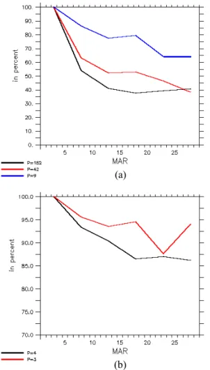
Adjustment errors E (t) computed at the parking depth in presence of this observa-tional error are presented in Fig. 9a for P=182, 42, 9. They can be compared with

15

the results in Fig. 4 obtained with perfect datasets. With low data coverage (P=9, 42), the evolution of E (t) is very close to that obtained with perfect datasets, with minimum values of 70% and 40% respectively obtained at the end of the assimilation period. In case of high data coverage (P=182), on the other hand, the E decrease is quickly re-duced after the third sequence. Its minimum is approximately 40%, while in the case of

20

perfect data E (t) reached 20%. This different behaviour can be explained considering that datasets of low coverage provide information of coarse resolution on the truth cir-culation, while shear errors have relatively small amplitudes and would affect only fine scale information. In consequence, the obtained velocity estimates for low coverage are likely to be less sensitive to the introduction of shear errors which only affect high

25

resolution datasets.

A second characteristic of Argo floats concerns their typical spatial coverage. For ex-ample, there are typically three to six active floats in the North Western Mediterranean

(20)

OSD

3, 255–289, 2006

Full Screen / Esc

EGU Sea in the framework of the MFSTEP project. So the simulated data sets have to be

reduced to few trajectories. Corresponding adjustment errors E (t) are represented in Fig. 9b for P=3 and P =4. E(t) decreases in average indicating that the assimilation is effective, but the evolution appears non monotonous, especially for P =3, with vari-ations between sequences of the order of 5%. Minimum E values reached during the

5

one month assimilation are between 85% and 95%.

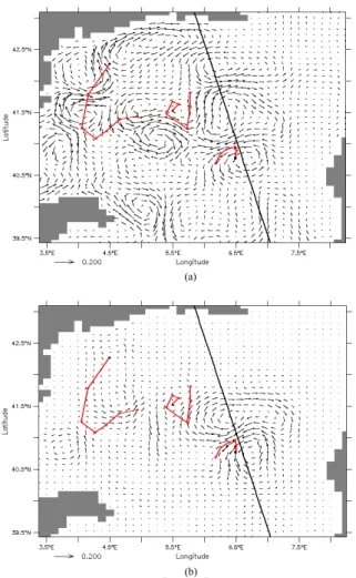
Such a global assessment needs to be refined in order to understand what could be expected in the assimilation of real Argo data positions. In order to have a more de-tailed, even though qualitative assessment, we consider a horizontal map at the parking depth of the truth minus background misfit (utru–ubck) at the end of the integration and

10

we compare it with the estimate minus background misfit (uest – ubck) obtained with

P=3. The corresponding fields and floats trajectories are shown in Fig. 10. A visual

comparison shows that the assimilation tends to reproduce correctly the main struc-tures, at least in the areas where data are available. The three floats sample different regions and have different impacts on the assimilation process. The most western float

15

is located in a very energetic area. It is therefore characterized by important displace-ments. The other two floats are located in a more quiescent region, with meandering motion and reduced displacements. For the energetic float, the structures of velocity corrections obtained at each sequence appear to propagate quickly south-westward, as indicated by the structure situated north of the Balearic Islands. The propagation is

20

likely to be due to a combination of advection processes and propagation of Rossby modes that are prominent in this area (Pinardi and Navarra, 1993). As a consequence, the velocity corrections which persist in the map (Fig. 10b) are mostly performed at the final sequences. Thus the global adjustment error E (t) quickly reaches its threshold value. For the less energetic floats in the central basin, on the other hand, the local

25

velocity correction appears less influenced by propagation. As the floats stay longer in the same zone, velocity estimates obtained at the end of the assimilation period re-sult from the whole sequences of analysis. Particularly, the eastern trajectory infers a major correction on the background circulation to relocate northward the flow path.

(21)

OSD

3, 255–289, 2006

Full Screen / Esc

EGU The trajectory located at the centre, which starts with slow displacements to finish with

larger ones, leads to velocity corrections partially propagating westward where they contribute to the correction inferred by the previous float. Another part of the correction does not appear to move, and it leads to a local correction which is not in complete agreement with the truth minus background misfit at the end of the assimilation period.

5

6 Summary and concluding remarks

An assimilation method for Argo float positions has been developed and implemented. Investigations have been performed in a realistic model configuration of the Mediter-ranean Sea focusing on the North Western area. A first set of experiments have been performed to test the method in ideal conditions. Perfect data with no shear error are

10

considered, corresponding to the initial and final positions of each cycle drift at the parking depth z_p. Relatively high coverages are considered, with a number of floats ranging between P=182 and P =9. Two different procedures are tested: a “state of art” one, where for each sequence the analysis is performed at initial time and the model is re-run forward starting from the corrected initial conditions; and an “operational” one

15

where the analysis is performed at final time and the model is not re-run forward on the sequence.

The results show that the assimilation is effective for both procedures. The velocity field estimated at z_p converges toward the truth at increasing coverage. The global adjustment error E , computed over the region of interest, ranges between 20% for

20

P=180 and 70% for P =9 after one month of assimilation. The correction projected in

the water column is effective in a thick intermediate layer around z_p. For deeper layers or lower coverage (P=9) the correction is lower but still significant, with values around

E=70%. Also the correction of the mass field TS appears significant and consistent,

even for low coverage. The performance of the two procedures is similar, provided that

25

the mass field is estimated as discussed in Sect. 2.2. Only when TS are not actively corrected (and let free to evolve and passively correct themselves), the “operational”

(22)

OSD

3, 255–289, 2006

Full Screen / Esc

EGU procedure appears significantly less effective. Given that the “operational” procedure

has a lower CPU cost and it is more compatible with standard procedures for the as-similation of other data sets, we consider it more convenient and we recommend it for future applications.

A second set of tests have been performed (with the “operational” procedure only)

5

using data with realistic characteristics, with the goal of investigating the potential im-pact of Argo floats in observing systems. Realistic position data are considered, i.e. taken at the surface and therefore contaminated by shear errors. The results are com-pared with those for perfect data with P=182, 42, 9. Accounting for shear errors shows a significant impact for high coverage, P=182, increasing the final adjustment from

10

E=20% to E=40%. For lower coverage, the impact appears negligible, possibly

be-cause its fine scale effect is masked by the coarse resolution of the datasets used to describe the truth circulation. We have then considered the impact of realistically low coverage, considering P=4, 3. The assimilation appears effective in the sense that the global adjustment error E (t) tends to decrease in average, even though its final

15

value is high, of the order of 85–95%. Locally, the assimilation effectively corrects the mesoscale structures sampled by the data. Even when the correction propagates dy-namically (through advection and wave propagation) in regions with no data, it correctly modifies the model circulation with respect to the truth. Of course, as for any sparse dataset, the possibility of having spurious corrections in regions of data voids persists,

20

but this phenomenon appears very limited at least in the performed experiments, pos-sibly because of the dynamically balanced nature of the correction.

In summary, the present results indicate that the assimilation of realistic Argo floats, despite shear error and sparseness, can provide significant corrections to model solu-tions and help converging toward the truth. These results are confirmed by a recent

25

work by Taillandier et al. (2006b), where in-situ Argo data from the MFSTEP project in the Mediterranean Sea have been assimilated in the OPA model in the same region considered here. In the case of in-situ data, results cannot be tested against the truth which is obviously unknown. Nevertheless, the corrections appear significant and

(23)

con-OSD

3, 255–289, 2006

Full Screen / Esc

EGU sistent with Argo float measurements and, at least qualitatively, also with independent

current-meter measurements.

We notice that an intrinsic limit to the use of Argo data positions is the fact that the time interval∆t between successive observations is of the order of T_L. This implies that the details on the structure curvature are not contained in the data. In the present

5

runs, we have not encountered any major problem related to this, differently from the previous work by Taillandier et al. (2006a) where floats in a strong vortex appeared to lead to spurious velocity corrections. This is probably due to the fact that in Taillandier et al. (2006a) the velocity field was reconstructed from float data alone, without as-similating them in a model, while here accounting for model dynamics helps providing

10

additional information on the structures. On the other hand, even though no catas-trophic event occurs in the present experiments, the float correction is in general less significant for structures of high curvature, such as small and intense vortices, with respect to circulation features with broader scales, such as major currents or mean-ders. This can be seen also in the assimilation of in-situ data (Taillandier et al., 2006b).

15

When the floats enter strong currents and jets with long time and space correlations, the velocity correction is strong and consistent, while when floats loop in small struc-tures such as submesoscale vortices (Testor and Gascard, 2003; Testor et al., 2005), the correction is weaker.

As a final remark we notice that, even though the present results are very positive,

20

some aspects persist that can be further investigated and improved in future works. First of all, we notice that the results strongly depend on the statistical correlations used for projection of the velocity correction in the water column. While in the North Western Mediterranean Sea considered here the velocity correlation profiles appear well represented, it can be expected that in regions with stronger variability and

baro-25

clinicity the approach might be less successful. Also, the use of the geostrophic bal-ance in the mass correction limits the validity of the method to mesoscale open ocean or shelf flows. In principle, a powerful alternative to the statistical projection and simpli-fied dynamics used here is a constraint based on the full model dynamics (e.g., Nodet,

(24)

OSD

3, 255–289, 2006

Full Screen / Esc

EGU 2006). The counterpart is that the number of variables and parameters to be fitted to

the data is much higher. So, for a reduced data set as for Argo floats, the choice of the most effective method is expected to be a compromise between the complexity of the considered dynamics and the type of available information.

Acknowledgements. This work was supported by the European Commission (V Framework

5

Program – Energy, Environment and Sustainable Development) as part of the MFSTEP project (contract number EVK3-CT-2002-00075) and by the Office of Naval Research grant N00014-05-1-0094. We wish to gratefully thank A. Bozec, K. B éranger, L. Mortier for their assistance, P. De Mey, A. Molcard, T. Özg ökmen for useful discussions. Thanks to the MERCATOR project which provided the numerical model and the forcing from ECMWF.

10

References

B ´eranger, K., Mortier, L., and Cr ´epon, M.: Seasonal variability of transports through the Gibraltar, Sicily and Corsica straits from a high resolution Mediterranean model, Progress in Oceanography, 66, 341–364, 2005.

Gilbert, J.-C. and Lemar ´echal, C.: Some numerical experiments with variable-storage

quasi-15

Newton algorithms, Mathematical Programming, 45, 407–435, 1989.

Ide, K., Kuznetsov, L., and Jones, C. K. R. T.: Lagrangian data assimilation for point vortex systems, J. Turbul., 3, doi:10.1088/1468-5248/3/1/053, 2002.

Ishikawa, Y. I., Awaji, T., and Akimoto, K.: Successive correction of the mean sea surface height by the simultaneous assimilation of drifting buoys and altimetric data, J. Phys. Oceanogr., 26,

20

2381–2397, 1996.

Jackett, D. R. and McDougall, T. J.: Minimal adjustment of hydrographic profiles to achieve static stability, J. Atmos. Ocean. Tech., 12, 381–389, 1995.

Kamachi, M. and O’Brien, J.: Continuous assimilation of drifting buoy trajectory into an equato-rial Pacific Ocean model, J. Marine Syst., 6, 159–178, 1995.

25

Kutsnetsov, L., Ide, K., and Jones, C. K. R. T.: A method for assimilation of Lagrangian data, Mon. Wea. Rev., 131, 2247–2260, 2003.

Madec, G., Deleucluse, P., Imbard, M., and Levy, C.: OPA8.1 ocean general circulation model reference manual, Technical Report LODYC/IPSL,http://www.lodyc.jussieu.fr/opa, 1998.

(25)

OSD

3, 255–289, 2006

Full Screen / Esc

EGU

Molcard, A., Griffa, A., and ¨Ozg¨okmen, T.: Lagrangian data assimilation in multilayer primitive equation models, J. Atmos. Ocean. Tech., 22, 70–83, 2006.

Molcard, A., Piterbarg, L. I., Griffa, A., ¨Ozg¨okmen, T., and Mariano, A. J.: Assimilation of drifter positions for the reconstruction of the eulerian circulation field, J. Geophys. Res., 108, 3056, doi:10.1029/2001JC001240, 2003.

5

Molcard, A., Poje, A. J., and ¨Ozg ¨okmen, T.: Directed drifter launch strategies for Lagrangian data assimilation using hyperbolic trajectories, Ocean Modelling, 12(3–4), 268–289, 2006. Nodet, M.: Variational assimilation of Lagrangian data in oceanography, Inverse Problems, 22,

245–263, 2006.

Oschlies, A. and Willebrand, J.: Assimilation of Geosat altimeter data into an eddy-resolving

10

primitive equation model of the North Atlantic Ocean, J. Geophys. Res., 101, 14 175–14 190, 1996.

¨

Ozg ¨okmen, T., Molcard, A., Chin, T. M., Piterbarg, L. I., and Griffa, A.: Assimilation of drifter positions in primitive equation models of midlatitude ocean circulation, J. Geophys. Res., 108, 3238, doi:10.1029/2002JC001719, 2003.

15

Park, J. J., Kim, K., King, B. A., and Riser, S. C.: An advanced method to estimate deep currents from profiling floats, J. Atmos. Ocean. Tech., 22, 1294–1304, 2005.

Pinardi, N. and Navarra, A.: Baroclinic wind adjustment processes in the Mediterranean Sea, Deep Sea Res. II, 40, 1299–1326, 1993.

Pinardi, N., Allen, I., Demirov, E., De Mey, P., Korres, G., Lascaratos, A., Le Traon, P.-Y.,

20

Maillard, C., Manzella, G., and Tziavos, C.: The Mediterranean ocean forecasting system: first phase of implementation (1998–2001), Ann. Geophys., 21, 3–20, 2003.

Poulain, P.-M.: MEDARGO: A profiling float program in the Mediterranean, Argonautics, 6, 2, 2005.

Raicich, F. and Rampazzo, A.: Observing system simulation experiments for the assessment

25

of temperature sampling strategies in the Mediterranean Sea, Ann. Geophys., 21, 151–165, 2003.

Taillandier, V., Griffa, A., and Molcard, A.: A variational approach for the reconstruction of regional scale Eulerian velocity fields from Lagrangian data, Ocean Modelling, 13(1), 1–24, 2006a.

30

Taillandier, V., Griffa, A., Poulain, P.-M., and B´eranger, K.: Assimilation of Argo float positions in the North Western Mediterranean Sea and impact on ocean circulation simulations, Geo-phys. Res. Lett., in press, 2006b.

(26)

OSD

3, 255–289, 2006

Full Screen / Esc

EGU

Talagrand, O.: A posteriori evaluation and verification of analysis and assimilation algorithms, Proceedings of workshop on “Diagnostic of data assimilation systems” ECMWF, 1999. Talagrand, O. and Courtier, P.: Variational assimilation of meteorological observations with the

adjoint vorticity equation, Q. J. Roy. Meteor. Soc., 113, 1311–1328, 1987.

Testor, P. and Gascard, J.-C.: Large-scale spreading of deep waters in the Western

Mediter-5

ranean Sea by submesoscale coherent eddies, J. Phys. Oceanogr., 33, 75–87, 2003. Testor, P., B ´eranger, K., and Mortier, L.: Modelling the eddy field in the South

West-ern Mediterranean: the life cycle of Sardinian eddies, Geophys. Res. Lett., 32, L13602, doi:10.1029/2004GL022283, 2005.

Toner, M., Poje, A. J., Kirwan, A. D., Jones, C. K. R. T., Lipphardt, B. L., and Grosch, C.

10

E.: Reconstructing basin-scale Eulerian velocity fields from simulated drifter data, J. Phys. Oceanogr., 31, 1361–1376, 2001.

(27)

OSD

3, 255–289, 2006

Full Screen / Esc

EGU

Figure 1. Correlation and regression profiles of velocity components between depths z and zp=350m.

Fig. 1. Correlation and regression profiles of velocity components between depths z and

z_p=350 m.

(28)

OSD

3, 255–289, 2006

Full Screen / Esc

EGU Figure 2. Details of a simulated Argo type trajectory. The high resolution trajectory is

shown, with superimposed the trajectory sampled at ∆t = 5 days, as observed at the surface. Crosses indicate positions where the simulated float reaches or leaves its parking depth.

Fig. 2. Details of a simulated Argo type trajectory. The high resolution trajectory is shown,

with superimposed the trajectory sampled at∆t=5 days, as observed at the surface. Crosses indicate positions where the simulated float reaches or leaves its parking depth.

(29)

OSD

3, 255–289, 2006

Full Screen / Esc

EGU Figure 3. Lagrangian description of the truth circulation utru during the month of March

1999. Three coverages with different number of trajectories P are represented: P = 182 (a), P = 42 (b), P = 9 (c). The locations of float deployment are indicated by a cross. The computational domain is bounded inside the box.

(a) (b)

(c)

Fig. 3. Lagrangian description of the truth circulation utru during the month of March 1999.

Three coverages with different number of trajectories P are represented: P =182 (a), P =42 (b),

P=9 (c). The locations of float deployment are indicated by a cross. The computational domain

(30)

OSD

3, 255–289, 2006

Full Screen / Esc

EGU

37

Figure 4. Evolution of the error E(t) at the parking depth computed from perfect data with three coverages P = 182, 42, 9, using the assimilation procedure “state of art” (a) and “operational” (b).

(a) (b)

Figure 4. Evolution of the error E(t) at the parking depth computed from perfect data with three coverages P = 182, 42, 9, using the assimilation procedure “state of art” (a) and “operational” (b).

(a) (b)

Fig. 4. Evolution of the adjustment error E (t) (in %) at the parking depth computed from perfect

data with three coverages P=182, 42, 9, using the assimilation procedure “state of art” (a) and “operational”(b).

(31)

OSD

3, 255–289, 2006

Full Screen / Esc

EGU

Figure 5. Velocity fields at the parking depth at the end of the assimilation period. The background circulation is represented in panel (a), the truth circulation in panel (b), and in panels (c) (d) the estimated circulation with the procedure “state of art” (“operational”) using 42 trajectories. The hydrologic section is drawn in straight line.

(a) (b)

(c) (d)

(a) (b)

(c) (d)

38

(a) (b)

(c) (d)

38

(a) (b)

(c) (d)

Fig. 5. Velocity fields at the parking depth at the end of the assimilation period. The background

circulation is represented in panel(a), the truth circulation in panel (b), and the estimated

circu-lation with the procedure “state of art” (“operational”) in panels(c) and (d) using 42 trajectories.

The hydrologic section is drawn as a straight line.

(32)

OSD

3, 255–289, 2006

Full Screen / Esc

EGU Figure 6. Profiles of E(z) at the end of the assimilation period for P = 182 (top), 42

(middle), 9 (bottom), for the procedure “state of art” (left) and “operational” (right). Adjustment errors of the vertical mean velocity are indicated in straight lines.

Fig. 6. Profiles of E (z) at the

end of the assimilation period for

P=182 (top), 42 (middle), 9

(bot-tom), for the procedure “state of art” (left) and “operational” (right). Adjustment errors of the vertical mean velocity are indi-cated in straight lines.