Stratospheric dryness

(1)

HAL Id: hal-00302265

https://hal.archives-ouvertes.fr/hal-00302265

Submitted on 14 Nov 2006

HAL is a multi-disciplinary open access

archive for the deposit and dissemination of sci-entific research documents, whether they are pub-lished or not. The documents may come from teaching and research institutions in France or abroad, or from public or private research centers.

L’archive ouverte pluridisciplinaire HAL, est destinée au dépôt et à la diffusion de documents scientifiques de niveau recherche, publiés ou non, émanant des établissements d’enseignement et de recherche français ou étrangers, des laboratoires publics ou privés.

Stratospheric dryness

J. Lelieveld, C. Brühl, P. Jöckel, B. Steil, P. J. Crutzen, H. Fischer, M. A.

Giorgetta, P. Hoor, M. G. Lawrence, M. Milz, et al.

To cite this version:

J. Lelieveld, C. Brühl, P. Jöckel, B. Steil, P. J. Crutzen, et al.. Stratospheric dryness. Atmospheric Chemistry and Physics Discussions, European Geosciences Union, 2006, 6 (6), pp.11247-11298. �hal-00302265�

(2)

ACPD

6, 11247–11298, 2006 Stratospheric dryness J. Lelieveld et al. Title Page Abstract Introduction Conclusions References Tables Figures ◭ ◮ ◭ ◮ Back Close

Full Screen / Esc

Printer-friendly Version Interactive Discussion

EGU

Atmos. Chem. Phys. Discuss., 6, 11247–11298, 2006 www.atmos-chem-phys-discuss.net/6/11247/2006/ © Author(s) 2006. This work is licensed

under a Creative Commons License.

Atmospheric Chemistry and Physics Discussions

Stratospheric dryness

J. Lelieveld1, C. Br ¨uhl1, P. J ¨ockel1, B. Steil1, P. J. Crutzen1,2, H. Fischer1, M. A. Giorgetta3, P. Hoor1, M. G. Lawrence1, M. Milz4, R. Sausen5, G. P. Stiller4, and H. Tost1

1

Max Planck Institute for Chemistry, J.J. Becherweg 27, 55128 Mainz, Germany 2

Scripps Institution of Oceanography, UCSD, La Jolla, CA 92093-0221, USA 3

Max Planck Institute for Meteorology, Bundesstrasse 53, 20146 Hamburg, Germany 3

FZK Institute for Meteorology and Climate Research, 76021 Karlsruhe, Germany 3

DLR-Institut f ¨ur Physik der Atmosph ¨are, Oberpfaffenhofen, 82234 Wessling, Germany Received: 20 October 2006 – Accepted: 9 November 2006 – Published: 14 November 2006 Correspondence to: J. Lelieveld (lelieveld@mpch-mainz.mpg.de)

(3)

ACPD

Full Screen / Esc

EGU

Abstract

The mechanisms responsible for the extreme dryness of the stratosphere have been debated for decades. A key difficulty has been the lack of models which are able to re-produce the observations. Here we examine results from a new atmospheric chemistry general circulation model (ECHAM5/MESSy1) together with satellite observations. Our 5

model results match observed temperatures in the tropical lower stratosphere and re-alistically represent recurrent features such as the semi-annual oscillation (SAO) and the quasi-biennual oscillation (QBO), indicating that dynamical and radiation processes are simulated accurately. The model reproduces the very low water vapor mixing ratios (1–2 ppmv) periodically observed at the tropical tropopause near 100 hPa, as well as 10

the characteristic tape recorder signal up to about 10 hPa, providing evidence that the dehydration mechanism is well-captured, albeit that the model underestimates con-vective overshooting and consequent moistening events. Our results show that the entry of tropospheric air into the stratosphere at low latitudes is forced by large-scale wave dynamics; however, radiative cooling can regionally limit the upwelling or even 15

cause downwelling. In the cold air above cumulonimbus anvils thin cirrus desiccates the air through the sedimentation of ice particles, similar to polar stratospheric clouds. Transport deeper into the stratosphere occurs in regions where radiative heating be-comes dominant, to a large extent in the subtropics. During summer the stratosphere is moistened by the monsoon, most strongly over Southeast Asia.

20

1 Introduction

The stratosphere between about 12±4 and 50 km altitude (between ∼150±50 and 1 hPa atmospheric pressure) receives much attention because it encompasses the ozone layer, being thinned by anthropogenic halocarbon gases. Even though the stratosphere is very dry compared to the troposphere, water is central in radiative and 25

(4)

ACPD

Full Screen / Esc

EGU

In the energy budget of the lower stratosphere the emission of thermal infrared (IR) radiation by H₂O is a main cooling term (Mlynczak et al., 1999). Further, H₂O chem-istry is the primary source of hydroxyl (OH) radicals, which initiate oxidation processes and destroy ozone (Solomon, 1999). Important oxidation reactions by OH include the release of ozone destroying halogen radicals from HCl and HBr, and the conversion 5

of CH4 into CO2 and 2H2O. The latter reaction is an important source of water in the middle and upper stratosphere, whereas in the lower stratosphere transport from the troposphere is prevalent (Remsberg et al., 1996). The common view is that strato-spheric air is moistened from about 2–4 ppmv H2O at the tropical entry to 5–6 ppmv at the extra-tropical exit at about 100 hPa (Kley et al., 2000). Despite the stratospheric 10

dryness, temperatures can be low enough for water to condense, for example, into polar stratospheric clouds. Heterogeneous reactions on these clouds and the sedi-mentation of ice particles play a key role in the formation of the ozone hole.

More than half a century ago Brewer (1949) explained the dryness of the strato-sphere by the large-scale ascent of air across the tropical tropopause, acting as a “cold 15

trap”. Owing to the negative temperature lapse rate in the troposphere, and the high and consequently very cold tropical tropopause, the air is “freeze-dried” at the strato-spheric entry. Although this general concept has been corroborated since (e.g. Holton et al., 1995), the locations and actual mechanisms controlling the freeze-drying have been subject of debate, spawned by the discovery of a water vapor minimum (hy-20

gropause) a few kilometers above the tropopause (Kley et al., 1979).

Two lines of explanation have evolved (Rosenlof, 2003). The first emphasizes the role of overshooting convection that penetrates the tropical tropopause and injects ice particles up to 18–20 km altitude (Danielsen, 1982; Sherwood and Dessler, 2001). Through sustained supersaturation cirrus clouds develop by the formation of new crys-25

tals or the growth of existing ones, which subsequently remove the moisture by grav-itational settling (sedimentation). The second focuses on particular fountain regions at the tropical tropopause where temperatures are very low so that cirrus clouds form during slow ascent and likewise desiccate the air by ice particle sedimentation (Newell

(5)

ACPD

Full Screen / Esc

EGU

and Gould-Stewart, 1981; Jensen et al., 2001).

Additional explanations have been pursued to reconcile the presence of deep con-vection below the tropopause and stratospheric dehydration aloft, for example, by as-suming convective excitement of gravity waves that propagate upward, cool the air in the wave crests and thus generate ice clouds (Potter and Holton, 1995), or by assuming 5

a combination of dehydration mechanisms (V ¨omel et al., 2002). Both the gradual up-welling and convective processes leave a distinct water vapor isotope ratio in the lower stratosphere, and measurements of hydrogen and oxygen isotopes in H2O have con-firmed that to some extent both mechanisms are involved (Webster and Heymsfield, 2003).

10

Satellite measurements from the early 1990s onward have greatly improved the time-height view of water vapor in the lower tropical stratosphere (Russell et al., 1993). Mote et al. (1996) have used these measurements to demonstrate the seasonal dependence of the freeze-drying effect, with coldest and driest tropopause conditions during boreal winter (December–March). They showed that the dehydration signal is carried deeper 15

into the stratosphere up to about 10 hPa, and dubbed this phenomenon the tropical tape recorder.

Here we present results of a new atmospheric chemistry general circulation model (AC-GCM) that describes the lower and middle atmosphere (Giorgetta et al., 2006; J ¨ockel et al., 2006). The global scale of the model precludes that we explicitly compute 20

convection and cloud microphysical details. Nevertheless, the model reproduces ob-served dynamical features and tracer distributions, including the tropical tape recorder. In the next section we review some main aspects of stratospheric radiation and dy-namics to provide a context for our AC-GCM simulation results and help understand the desiccation mechanism. Subsequently we present our model and the satellite data 25

used, comparisons of the different datasets and their interpretation, and we address the role of features that are not resolved by our AC-GCM. Finally we summarize the processes that control the dryness of the stratosphere.

(6)

ACPD

Full Screen / Esc

EGU

2 Stratospheric dynamics and radiation

The stratospheric circulation is driven by the following main forces. Firstly, the differen-tial solar heating of the stratospheric ozone layer in the winter hemisphere, i.e. between high latitudes in polar night and sunlit latitudes, causes large meridional temperature differences and hence poleward pressure forces. The additional effect of the Coriolis 5

force on the rotating Earth generates the polar vortices in the stratosphere.

Secondly, extra-tropical wave disturbances, excited in the troposphere by land-sea contrasts, flow over mountains and synoptic weather systems, may propagate into the stratosphere and exert a drag force onto the circumpolar westerlies. This deceleration of the polar vortex alters the balance between the pressure gradient and Coriolis forces, 10

which induces a residual meridional circulation towards the winter pole and a sinking motion in high latitudes (Haynes et al., 1991). Differences in the land-sea distribution and orography cause stronger wintertime wave effects on the stratospheric vortex in the Northern Hemisphere (NH) than in the Southern Hemisphere (SH).

The stratospheric mass balance is maintained by ascent near the equator, analogous 15

to a fluid-dynamical suction pump drawing air upward and poleward from the tropical tropopause at about 100 hPa (∼16 km altitude) (Holton et al., 1995). In the tropical mid-dle and upper stratosphere the upwelling is augmented by solar short-wave radiative heating (via O₃) although this is partly balanced through IR cooling by CO₂ and O₃ (Mlynczak et al., 1999). In the tropical lower stratosphere IR cooling by H2O is largely 20

compensated by IR heating by O3 so that on average net heating/cooling rates are small (Gettelman et al., 2004a). In fact, net radiative heating or cooling in the lower stratosphere is generally less than 1 K/day. The IR radiative effects of O3 and H2O have a pronounced spatial distribution (Highwood and Hoskins, 1998; Norton, 2001), and our model results presented below show that regional differences substantially 25

influence troposphere-to-stratosphere transport.

It is important to distinguish a transition region between the tropical troposphere and stratosphere between about 14 and 18 km altitude (i.e. about 150 and 75 hPa),

(7)

ACPD

Full Screen / Esc

EGU

called the tropical tropopause layer (TTL) (Highwood and Hoskins, 1998; Folkins et al., 1999). It has been proposed to define the TTL more accurately in terms of net radiative heating, but we argue against it because both the sign and the magnitude of this term vary strongly with the presence of cumulonimbus anvils and cirrus clouds. The latter can be found throughout the depth of the TTL (Wylie and Wang, 1997; Dessler et al., 5

2006) and have a profound impact on the heating profile (Hartmann et al., 2001; Corti et al., 2006).

By and large, upward motion below the TTL is governed by cumulonimbus convec-tion, whereas above the TTL it is controlled by extra-tropical wave dynamics. Thus both for the troposphere and the stratosphere the relevant process understanding is well es-10

tablished, whereas for the TTL the picture is less unambiguous. This partly results from the fact that vertical velocities in the TTL are small and difficult to measure, especially above extensive cumulonimbus anvils. Furthermore, it is clear that the initial impact of cumulonimbus convection is moistening because these clouds carry saturated air and condensates into the upper troposphere and TTL (Soden, 2004; Luo and Rossow, 15

2004). Therefore, an explanation of stratospheric dryness will need to reconcile the direct moistening and indirect dehydration attributes of convection.

The coldest parts of the TTL are found over the areas with most extensive deep convection, notably over the western Pacific Ocean warm pool (Seidel et al., 2001). In these cold regions thin cirrus clouds can be formed, also known as subvisual or 20

subvisible cirrus (Wylie and Wang, 1997). These ice clouds can desiccate the air by ice particle sedimentation (Jensen et al., 2001), and our model results presented below show that this process is most efficient between 200 and 100 hPa.

Here we focus on the geographic region where upward motion predominates in the lower stratosphere, between 30◦N and 30◦S latitude (Rosenlof, 1995). We consider 25

the ten year period 1996–2005 for which model calculations have been performed and satellite data are available. The pressure altitudes on which we concentrate our model evaluation are 100 hPa, approximately representing the tropopause in the middle of the TTL, and 70 hPa, just above the TTL where dehydrated air enters into the stratosphere.

(8)

ACPD

Full Screen / Esc

EGU

3 Numerical model

The atmospheric chemistry GCM used in our study couples the 5th generation Eu-ropean Centre – Hamburg model, ECHAM5 (version 5.3.01) (Roeckner et al., 2003, 2006) to the 1st Modular Earth Submodel System, MESSy1. This model – abbreviated E5M1 – includes a comprehensive representation of tropospheric and stratospheric 5

cloud, radiation, multiphase chemistry and emission-deposition processes (J ¨ockel et al., 2006). The model has a spectral dynamical core, computing the atmospheric dy-namics up to wave number 42 using a triangular truncation (T42), while physical and chemical parameterizations are calculated on the associated quadratic Gaussian grid at a resolution of about 2.8◦ in latitude and longitude (Roeckner et al., 2006).

10

The vertical grid used here resolves the lower and middle atmosphere with 90 vertical layers from the surface to a top layer centered at 0.01 hPa (∼80 km altitude). The mean layer thickness in the lower and middle stratosphere is about 700 m, sufficient to resolve vertically propagating waves with vertical wavelengths of 2.8 km and longer, which is a prerequisite to realistically simulate the quasi-biennial oscillation (QBO) (Giorgetta et 15

al., 2006). In the upper troposphere and lower stratosphere the vertical resolution is about 500 m (6–10 hPa).

Prognostic variables, predicted on the basis of fundamental (primitive) equations in spectral space, i.e. temperature, divergence, vorticity, (the logarithm of) surface pres-sure, and those in grid point space such as specific humidity, cloud liquid and ice water 20

and chemical tracers, are calculated every 15 min (at T42 resolution). Orographic and non-orographic gravity waves are parameterized (Manzini and McFarlane, 1998), as used in a previous chemistry-climate version of the model (Manzini et al., 2003; Steil et al., 2003). Details of the model setup are provided in J ¨ockel et al. (2006); note that we use the S2 model setup described in that article.

25

ECHAM5 has been coupled with MESSy1, which comprises a modular interface structure that connects submodels to the dynamical core model (J ¨ockel et al., 2005; see also http://www.messy-interface.org). The tracer advection is calculated with a

(9)

ACPD

Full Screen / Esc

EGU

mass conserving flux form semi-Lagrangian scheme (Lin and Rood, 1996). The ECHAM5 radiation scheme distinguishes four UV-VIS and near-IR, and 16 thermal IR spectral regions (Wild and Roeckner, 2006), and it utilizes the online computed tracer distributions. Photolysis rate calculations for the troposphere up to the mesosphere are based on the eight spectral band approach described in (Landgraf and Crutzen, 1998), 5

considering absorption and scattering by gases, aerosols and clouds in a delta-two-stream method.

Detailed chemistry calculations are performed using a kinetic preprocessor (Sandu and Sander, 2006), applying a Rosenbrock solver, to describe a set of about 200 gas phase, 70 photo-dissociation and 85 heterogeneous tropospheric and stratospheric 10

reactions (Sander et al., 2005). Details of the chemical mechanism (including reaction rate coefficients and references) can be found in the electronic supplement of Sander et al. (2005) (http://www.atmos-chem-phys.net/5/445/2005/acp-5-445-2005-supplement.

zip).

For the representation of natural and anthropogenic emissions and dry deposition of 15

trace species, including micrometeorological and atmosphere-biosphere interactions, wet deposition by large-scale and convective clouds, multiphase chemistry and polar stratospheric clouds, we refer to the detailed descriptions by Ganzeveld et al. (2006), Kerkweg et al. (2006a, b) and Tost et al. (2006a, b). The results of the tropospheric and stratospheric chemistry calculations, using a number of diagnostic model routines, 20

have been tested against in situ and satellite measurements (J ¨ockel et al., 2006). Cloud convection is described using the method presented in Tiedke (1989), which assumes that an ensemble of clouds modifies the large-scale environmental dry static energy and specific humidity. The scheme distinguishes three types of convection (Roeckner et al., 2003): i) Penetrative, deep convection, triggered by convergence in 25

the boundary layer, in which entrainment is proportional to the large-scale moisture convergence; ii) Shallow convection, mostly triggered by subcloud layer turbulence; and iii) Midlevel convection originating at higher altitudes, e.g. frontal clouds in extra-tropical cyclones, where the cloud base and entrainment are determined by the

(10)

large-ACPD

Full Screen / Esc

EGU

scale flow.

An addition to the convection routine by Nordeng (1994) accounts for organized entrainment/detrainment in deep convection, and mass closure based on convective available potential energy. An intercomparison of different convection schemes in ECHAM5 has shown that the present model setup produces a realistic hydrological 5

cycle, including clouds, precipitation and water vapor distribution in the upper tropo-sphere and lower stratotropo-sphere (Tost et al., 2006b). The convective tracer transport calculations use a monotonic, positive definite and mass conserving algorithm follow-ing a bulk approach (Tost, 2006).

The model scheme for stratiform clouds includes prognostic equations for liquid and 10

ice water and for the higher order moments of total cloud water (Roeckner et al., 2003). The description of cloud physics includes rain formation by coalescence, the aggrega-tion of ice crystals into snowflakes, accreaggrega-tion of cloud droplets by falling snow, gravita-tional settling of hydrometeors and phase transition processes (Lohmann and Roeck-ner, 1996). Between 238 K and 273 K a mixed cloud phase is assumed, whereas at 15

lower temperatures the condensed water is in the form of ice only. At temperatures below 238 K all cloud water freezes instantaneously.

The parameterizations of cloud micro-physical processes are relatively detailed for a GCM, and include condensation/evaporation of liquid water, deposition/sublimation of ice, evaporation of rain, sublimation of snow, autoconversion of cloud droplets, accre-20

tion of cloud droplets by precipitation, homogeneous, stochastical-heterogeneous and contact freezing of droplets, and aggregation of ice crystals and melting of cloud ice (Lohmann and Roeckner, 1996). A description of the ECHAM5 simulated hydrological cycle is presented in Hagemann et al. (2006).

The growth of ice crystals below temperatures of 238 K takes place by the deposition 25

of water vapor. It is assumed that slow air parcel ascent in cold clouds occurs at ice saturation. At temperatures above 238 K water vapor deposition only takes place if cloud ice is already present. The size distribution of ice crystals is based on an empirical relationship between the effective particle radius of the ice crystal distribution

(11)

ACPD

Full Screen / Esc

EGU

and the ice water content derived from aircraft observations. The sedimentation of ice particles is also parameterized through an empirical description, representing observed ice mass precipitation rates (Heymsfield and Donner, 1990). The model calculated mean ice water content of cirrus clouds over the equatorial Pacific Ocean compare well with ice measurements in the 205–270 K temperature interval (Lohmann et al., 5

1995; McFarquhar and Heymsfield, 1996).

In order to analyze the transport fluxes of air and water in its different phases, we apply the ATTILA Lagrangian transport scheme (Reithmeier and Sausen, 2002), for which the model atmosphere is subdivided into about 1 700 000 air parcels of constant mass (ATTILA: Atmospheric Tracer Transport In a Lagrangian model). The scheme 10

applies a fourth order Runge-Kutta method for advection, and we employ it diagnos-tically as an on-line forward trajectory model. The results of this method have been tested against a trajectory model using data of the European Centre for Medium-range Weather Forecasts (ECMWF) (Stohl and Trickl, 1999; Traub, 2004).

The online coupling of the ATTILA transport scheme into our AC-GCM prevents time 15

interpolation errors typical for trajectory models, and it is fully mass conserving. Each of the computed forward trajectories has a “clock” to determine the moment at which a certain boundary is surpassed. The selected boundaries are the 200, 100 and 75 hPa pressure levels in our AC-GCM. Since two-way transport can occur over such bound-aries, we apply a residence time criterion of 96 h to define an exchange event as “al-20

most irreversible” (Wernli and Bourqui, 2002).

4 Model nudging

GCMs can be applied to simulate atmospheric conditions over extended periods, and the results of such simulations can be statistically compared with climatologies based on long-term observations or to other model simulations. For atmospheric chemistry 25

and stratospheric water vapor computations this is more difficult because extended data sets are rare, and it is more challenging to apply statistical techniques in model

(12)

ACPD

Full Screen / Esc

EGU

validation. Therefore, we follow the strategy of nudging the model toward realistic meteorological conditions, so that an evaluation of model results against observations is less dependent on the size of the datasets and a direct comparison becomes more meaningful.

The model has been nudged towards analyzed meteorological conditions for the pe-5

riod 1996–2005, based on ECMWF operational forecast analyses, by adding a Newto-nian relaxation term to the four above mentioned prognostic variables in spectral space, i.e. vorticity, divergence, temperature and surface pressure (Van Aalst et al., 2004). Several precautions prevent the excitement of spurious waves. Firstly, the ECMWF data are projected onto the model levels and surface orography by a interpolation pro-10

cedure developed by I. Kirchner, Free University of Berlin (personal communication), based on the method described in Majewski (1985). Secondly, the nudging strengths are very low (about 10−5s−1), with a 6 h relaxation e-folding time for vorticity, 12 h for temperature and surface pressure and 48 h for divergence. Thirdly, a slow-normal-mode filter is applied to the nudging data, which removes the fast components (Daley, 15

1991).

Finally, we avoid inconsistencies between the ECHAM5 and the ECMWF boundary layer representations by leaving the lowest three model levels free (apart from surface pressure), while the nudging increases stepwise in four levels up to about 706 hPa. The nudging tapers off to zero at 204 hPa to allow unconstrained simulations of the 20

TTL and stratosphere. From the perspective of the present study, the T42/2.8◦ and 90 layer resolution of the model is sufficiently high for the TTL and upward, though relatively low for the troposphere. The latter limitation is made up for by nudging the tropospheric part of the model using ECMWF data, which have been computed at much higher resolution.

25

We emphasize that it is important not to nudge the parameters and processes that di-rectly control water vapor and chemical tracers, and only optimize boundary conditions for the model-data comparison. Since the nudging is weak, the model reproduces the actual meteorology approximately but not exactly, so we still need to rely on some

(13)

sta-ACPD

Full Screen / Esc

EGU

tistical comparison with measurement data. Below we will compare probability density functions from model output and satellite measurements of stratospheric water vapor.

Figure 1 presents the results of the 10-year E5/M1 simulation used in the present study, showing that the model realistically simulates the Semi-Annual Oscillation (SAO), the QBO and the stratospheric tape recorder. A comparison with measured 5

tropical wind reversals in the QBO is presented by J ¨ockel et al. (2006), for a model version without chemistry by Giorgetta et al. (2006), and additional evaluation against satellite observations is presented below. These simulation results are available on request, and we provide a user-friendly web-based graphics tool to select data for geographical regions and time periods, and to download or plot the data in different 10

coordinates(http://airdata.mpch-mainz.mpg.de).

5 Satellite data

A long time series of stratospheric water vapor measurements is available from the Halogen Occultation Experiment (HALOE) on the Upper Atmospheric Research Satel-lite (UARS) (Russell et al., 1993). The instrument operated from the fall of 1991 until 15

the end of 2005, thus providing an extensive data set to compare with our model sim-ulations for the 1996–2005 time period. The comparison between model and satellite data focuses on 1997–2005, thus omitting 1996, because the first year is too close to the initial conditions of the model, based on HALOE data over the five years prior to the simulation period.

20

HALOE was a solar occultation limb sounder operating in the near-IR; water vapor was measured in the 6.6 µm channel. An advantage of solar occultation instruments is that a relative measurement is performed, i.e. the ratio between solar radiation out-side the atmosphere and that minus atmospheric attenuation. This technique may be conceived as self-calibrating and suffers little from instrument drifts, which is particu-25

larly useful for long-term observations. HALOE provided global coverage in the strato-sphere and mesostrato-sphere at a vertical resolution of about 2 km, with a total accuracy

(14)

ACPD

Full Screen / Esc

EGU

within about ±10% over much of the height range and decreasing to ±30% near the tropopause (Harries et al., 1996). A disadvantage of HALOE was that the number of measured profiles was relatively small, and global coverage was only achieved within about a month.

The second satellite instrument of which we use data is the Michelson Interferometer 5

for Passive Atmospheric Sounding (MIPAS) on the European Environmental Satellite (ENVISAT). MIPAS is a high-resolution Fourier transform spectrometer, a limb scan-ning sounder operating in the near- and mid-IR, i.e. 4.15–14.6 µm (Fischer and Oelhaf, 1996). The instrument is operational since the fall of 2002, and provides global cover-age with 14–15 orbits per day at a horizontal resolution of 300–500 km and a vertical 10

resolution of about 3 km. Here we use MIPAS data for the period December 2002– November 2003. The potential bias of temperature measurements in the 10–35 km height interval has been assessed to be smaller than 0.5 K (Wang et al., 2005), with a total accuracy of individual data points (given as the square root of the quadratic sum of random and systematic errors) of 0.5–1.5 K. The water vapor retrieval yields a vertical 15

resolution of 4.5–6.5 km, and the total accuracy is within ±6–9% in the stratosphere, and up to about ±30% near the tropopause (Milz et al., 2005). The ozone data used are accurate to within about ±0.4 ppmv between 15 and 50 km altitude (Glatthor et al., 2006).

Finally, we use data from the Atmospheric Infrared Sounder (AIRS) on the NASA 20

Aqua satellite (Aumann et al., 2006). This is a nadir scanning grating-array spectrom-eter, which measures in the 3.7–15.4 µm spectral region in >2000 spectral channels at a horizontal resolution of 50 km and a vertical resolution of 1–2 km from the surface up to the lower stratosphere. The instrument is operational since summer 2002. A comparison of AIRS temperature data with balloon sounding and in situ aircraft mea-25

surements in the upper troposphere and lower stratosphere indicates a total accuracy within ±1.5 K near the tropopause (Gettelman et al., 2004b; Divakarla et a., 2006).

(15)

ACPD

Full Screen / Esc

EGU

6 Results and discussion

6.1 Middle and upper stratosphere

Figure 1 shows the model calculated zonal wind in the equatorial stratosphere (top) and zonal mean water vapor concentrations between 10◦N and 10◦S latitude (bottom). The computed water vapor mixing ratios compare favorably with HALOE measure-5

ments, although the model has a slight dry bias (Fig. 2), as discussed in more detail in subsequent sections. Since the magnitude of this bias is similar to the total accuracy of the satellite measurements and data retrieval, it seems reasonable to qualify this as good agreement.

In earlier studies it has been discussed that the signal of the QBO can be identified 10

in tracer distributions, including ozone and water vapor (Randel et al., 1996; Giorgetta and Bengtsson, 1999; Geller et al., 2002). The QBO modulates the upward velocity of air in the tropical stratosphere, and the temperature signal can modify the specific humidity. Therefore, the accurate simulation of the QBO is required to realistically compute the tape recorder signal in water vapor (Giorgetta et al., 2006). Nevertheless, 15

from Fig. 1, i.e. by comparing the upper and lower panels, the role of the QBO in the water vapor distribution is not clearly evident.

Closer inspection reveals that during the easterly phase at about 10 hPa the dry tongues reach to somewhat higher altitudes than during the westerly phase. In an earlier model version the upward penetration of moist air seemed deeper during the 20

easterly phase (Giorgetta and Bengtsson, 1999). However, in this earlier work the oxidation of methane was not considered, and it appears that during the westerly phase methane derived moisture is conveyed downward more efficiently from the mesosphere than in the easterly phase, which counteracts the QBO modulation of water vapor from below.

25

Interestingly, a rather strong influence is manifest from the SAO, where the westerly phase coincides with the most humid conditions. In our model results for the upper stratosphere we identify relatively narrow water vapor troughs in January and July and

(16)

ACPD

Full Screen / Esc

EGU

somewhat wider peaks in April and October, possibly a few weeks earlier than seen in satellite data during the period 1992–1995 (Jackson et al., 1998). The troughs are strongest in boreal winter, and they progress downward with a few hPa/month. It is also interesting to note in Fig. 1 that the westerly phase of the QBO starts after the west-erly phase of the SAO has progressively reached lower altitudes in the stratosphere, 5

indicating that the SAO plays a role in triggering the QBO.

In the middle and upper stratosphere there is a clear relationship between dryness and the easterly phase of the SAO, during which tropical dehydrated air is transported upward more efficiently. The relatively large interannual variability in the easterly phase coincides with relatively large variability in water vapor, whereby the lowest water vapor 10

mixing ratios occur during the strongest easterlies. Conversely, during the downward propagation of the westerly phase upward transport of dry air is reduced.

6.2 Lower stratosphere

Although the long time-span of the HALOE data series is unique, for the lower tropical stratosphere the comparison between modeled and measured water vapor is ham-15

pered by the sparseness of satellite observations. The HALOE water vapor retrieval is affected by thin cirrus cloud “contamination”, and since these clouds occur in very cold regions of active dehydration, as discussed in the next section, it is conceivable that the data are biased. Furthermore, by interpolating sparse HALOE data to display long-term tendencies, as shown in Fig. 2, the variability and seasonal cycle of water 20

vapor, being particularly strong near 100 hPa, are suppressed.

To circumvent these problems, we performed a direct comparison between both data sets by sampling the model results (from 5 hourly output) as closely as possible to the location and time periods of the HALOE measurements. We reiterate that we cannot expect that the applied nudging procedure leads to an exact mimicking of the synoptic 25

variability, and we must also accept sampling errors related to the different resolutions of the data sets. Nevertheless, it may be expected that such errors are relatively minor and appear as random noise in the statistical analysis.

(17)

ACPD

Full Screen / Esc

EGU

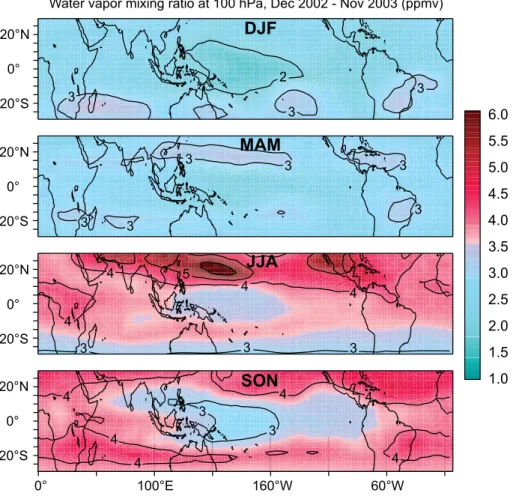
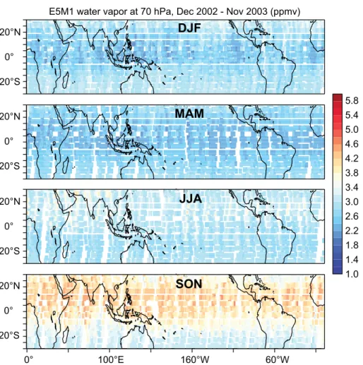
In Fig. 3 we show model calculated water vapor mixing ratios at the level nearest to 100 hPa (97 hPa) for four seasons during the period December 2002 to November 2003. These images are qualitatively consistent with previous analyses, e.g. of HALOE data by Randel et al. (2001), although these authors studied an earlier time period. The lowest water vapor mixing ratios are found over the equatorial western Pacific Ocean 5

during boreal winter (DJF), with a secondary minimum over the eastern Pacific and Central America. Highest water vapor mixing ratios, on the other hand, are found further north during boreal summer (JJA) over southern Asia, Central America and in particular over the western Pacific Ocean near 20◦N.

In the lower stratosphere water vapor strongly influences the local energy budget 10

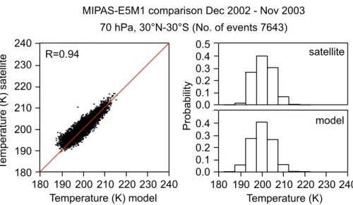
through IR radiative cooling, and temperature is also sensitive to dynamic processes through adiabatic expansion and cooling by the wave driven large-scale ascent. Fig-ure 4 shows that the model calculated temperatFig-ures agree excellently with the MIPAS measurements during the same period. The left panel in Fig. 4 shows a correlation plot (correlation coefficient R=0.94).

15

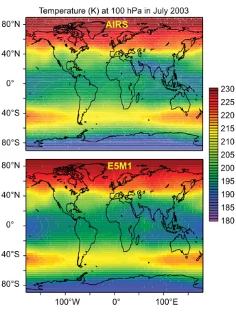
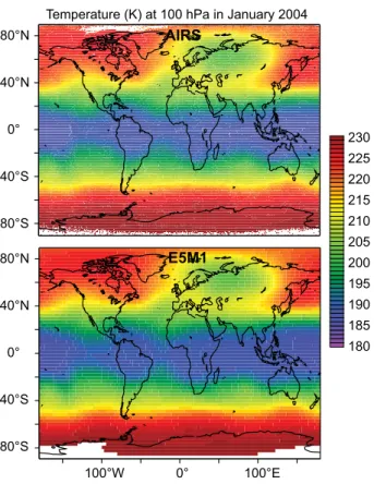
In the right panels we present the probability density functions (PDFs) of the model results and MIPAS data. The comparison of model results with AIRS temperature data is shown in Fig. 5, which corroborates the good agreement. We emphasize that MIPAS temperature data have a bias of less than 0.5 K, and both MIPAS and AIRS tempera-ture measurements have a total accuracy within ±1.5 K. The accurate simulation of the 20

temperature distribution is unlikely to be coincidental, and we interpret it as confirma-tion that the model realistically simulates dynamic and radiaconfirma-tion processes.

The water vapor minima and maxima in Fig. 3 coincide with regions of lowest and highest temperatures, respectively (Seidel et al., 2001). It is known that there is a strong correlation between water vapor and temperature near the tropical tropopause, 25

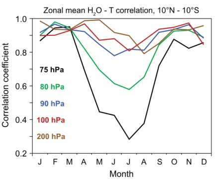
in line with the cold trap concept (e.g. Randel et al., 2004). In Fig. 6 we investigate this correlation for the inner tropics (10◦S–10◦N) in our model results. The correlation coefficient is generally high year around for the pressure levels 200–90 hPa, R≥0.8, and it is highest in boreal winter when dehydration in the equatorial zone is particularly

(18)

ACPD

Full Screen / Esc

EGU

effective.

From April to September the correlation coefficient is lower, especially at 80 and 75 hPa, and it breaks down to R≤0.4 at 75 hPa during June–August. This is the time of year during which the TTL is strongly influenced by water vapor intrusions from the Asian monsoon (discussed in Sects. 6.4–6.5). Particularly in the upper TTL the cor-5

relation between water vapor and temperature between 10◦S and 10◦N during boreal summer diminishes because the processes that control water vapor are to a large de-gree located in the outer tropics.

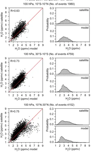
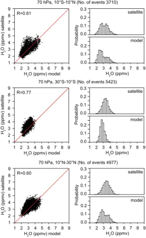
In Figs. 7 and 8 we compare the model results with HALOE water vapor data for the period 1997–2005 at the pressure levels 100 and 75 hPa, respectively. Both figures 10

indicate that especially the lowest water vapor mixing ratios are simulated accurately, indicating that our model reproduces the dehydration mechanism. Both the model and satellite data show that occasionally very low mixing ratios can occur at ∼100 hPa, down to nearly 1 ppmv. The correlation coefficients between both data sets for the three latitude bands shown are quite high, 0.63≤R≤0.75.

15

Again, the right panels show the PDFs, providing support for the good agreement at the low end of the water vapor distributions. The relatively large widths of the distri-butions indicate substantial variability, which seems to be underestimated in the model results. Especially toward the high end, above 3.5 ppmv, our model is too dry and the simulated PDFs typically peak ∼0.5 ppmv earlier than in the measurements. Although 20

the satellite data uncertainty is about ±30% for the lower stratosphere, the systematic nature of the model-measurement difference suggests that our model underestimates events of relatively high humidity, leading to a mean dry bias of approximately 0.5 ppmv. The lower left panel of Fig. 7 indicates that in some cases relatively high mixing ratios are calculated in locations that are much dryer in the observations, which could 25

be related to sampling errors or time shifts between computed and real events of high humidity at ∼100 hPa. Both in the model results and satellite data, the PDFs are wider at 10◦N–30◦N than at 10◦S–30◦S, a result of more frequent intrusions of high humidity associated with the Asian monsoon. The PDF for the inner tropics at 10◦S–10◦N,

(19)

ACPD

Full Screen / Esc

EGU

shown in the upper panel, is intermediate between both hemispheres.

The model-measurement correlation plots and PDFs for 70 hPa in Fig. 8 are com-pacter and narrower than for 100 hPa, respectively. The agreement is rather good, although the correlation coefficients are slightly lower than for 100 hPa, 0.60≤R≤0.77. The very low water vapor mixing ratios seen at 100 hPa are rare at 70 hPa, and data 5

points below 2 ppmv are absent. This may indicate that the strongest dehydration at ∼100 hPa takes place in air parcels that undergo intense radiative cooling, which in-duces their return to the troposphere (Sects. 6.4–6.5).

The variability is generally less at 70 hPa as a result of zonal and meridional mixing in the upper TTL. Both the correlation plots and PDFs show best agreement toward 10

low mixing ratios, and also reveal a small though significant dry bias in the upper part of the range. In the inner tropics at 10◦S–10◦N, shown in the upper panel of Fig. 8, the satellite measurements suggest a bimodal PDF, a consequence of moist events from higher latitudes. The model PDF verges upon this bimodality; however, the peak at ∼3.5 ppmv is underrepresented.

15

In Fig. 9 the E5M1 calculated water vapor mixing ratios at 70 hPa are compared with MIPAS observations, and the model results are displayed at the locations of the model grid cells closest to the satellite tracks. The most significant difference between Figs. 9a and b is that the satellite observations show a higher spatial and seasonal variability. The mean differences are nevertheless small, generally within ±15%. The 20

comparison corroborates that the model underestimates events of enhanced humidity in the outer tropics, in particular in the summer hemispheres.

In Fig. 10 we furthermore show a comparison of ozone mixing ratios between our model results and satellite observations between 30◦S and 30◦N at 70 hPa. The upper panels refer to the HALOE data for the 1997–2005 period, and the lower panels to the 25

MIPAS data for the December 2002–November 2003 period. The PDFs are similarly skewed in the model results and satellite data, both from HALOE and MIPAS, and the model-data correlations are rather high, R≥0.74, indicating that the model generally reproduces transport and chemistry. However, the computed ozone is systematically

(20)

ACPD

Full Screen / Esc

EGU

somewhat higher than the measurements, which points to a similar deficiency as the model dry bias.

Although the satellite measurement error for low O3mixing ratios (<1 ppmv) is rela-tively large, it nevertheless appears that our model does not reproduce the very low O3 events occasionally observed by both MIPAS and HALOE (see the lower left corners of 5

the left panels of Fig. 10 and the left wings of the PDFs). The likely reason is that our model underestimates convective intrusions of tropospheric air into the tropical lower stratosphere. Owing to the stability of the TTL, our model does not simulate convective overshooting beyond 100 hPa (Tost et al., 2006b), although in reality a small fraction of deep cumulonimbus clouds is so vigorous that they actually reach deeply into the up-10

per TTL (Alcala and Dessler, 2002). As a result, convective overshooting from time to time injects relatively ozone-poor and humid air across the tropical tropopause, which is subsequently carried into the lower stratosphere. Indirectly, this suggests that deep convective intrusions moisten the lower stratosphere.

6.3 Dehydration mechanism 15

Our model results show that water vapor mixing ratios at the tropical tropopause are not zonally uniform (Fig. 3), although the differences vanish upward through transport and mixing. The lower stratosphere is generally driest in the Indo-Pacific region during NH winter. The temporal and vertical distribution of “dryness” in Fig. 11 clearly shows the lowest mixing ratios during the December–March period.

20

Figure 11 includes the accompanying temperature distribution, illustrating that the driest regions (<2.5 ppmv) are also the coldest (<192 K). Furthermore, Fig. 11 demon-strates that the water vapor minimum is often most distinct at 75 hPa, well above the tropopause, consistent with the observed hygropause. Figure 11 also reveals that dur-ing NH winter the water minima ascend from 100 to 75 hPa in about a month, i.e. at a 25

mean speed of a few m/hour.

The tropical upwelling is brought about from above by the extra-tropical wave forc-ing, which has a maximum during December–March. Through adiabatic expansion

(21)

ACPD

Full Screen / Esc

EGU

and consequent cooling it contributes to the low tropopause temperatures (Yulaeva et al., 1994). In the region beneath, the deep tropical convection produces anvil clouds that moisten the upper troposphere through the evaporation of condensate, and the air is subsequently desiccated as it slowly travels through the TTL, as indicated by ob-servational and Lagrangian modeling studies (V ¨omel et al., 2002; Jensen and Pfister, 5

2004).

The ascent through the TTL is thus accompanied by adiabatic and radiative cooling, which together can be sufficient to maintain a high relative humidity and sustain water condensation on upward advected particles. Our model results indicate that net radia-tive cooling up to several K/day is prevalent below the TTL at ∼200 hPa throughout the 10

year, while it decreases with altitude within the TTL. If the radiative cooling would be stronger it could balance the wave driven ascent and even induce subsidence.

With increasing altitude in the TTL the O3 concentration and the consequent radia-tive heating increase; however, the thick convecradia-tive clouds below block the IR and O₃ heating so that freezing conditions are maintained. As a result of sustained supersat-15

uration over ice within certain regions of the TTL, thin cirrus clouds arise above the convective anvils, partly through the upward advection of ice crystals. Although the presence of tropopause cirrus clouds has been confirmed by aircraft measurements (McFarquhar et al., 2000; Thomas et al., 2002; Peter et al., 2003), it cannot be deter-mined with confidence to what degree they are remnants of anvils or are formed within 20

the TTL; in our model both are possible.

Figure 12 presents the model calculated mean ice water mixing ratios within the TTL. This tropopause cirrus, which represents a mean water mixing ratio of about 0.1 ppmv at 100 hPa, largely collocates with deep convection, in agreement with satellite mea-surements (Wylie and Wang, 1997; Massie et al., 2002; Dessler et al., 2006). As long 25

as the cirrus clouds overlie their cold cumulonimbus parents they contribute to radia-tive cooling. However, after the cumulonimbus anvils decay, the thin ice clouds become subjected to IR from the lower and warmer troposphere; hence, radiative heating in-tensifies and accelerates the transport into the stratosphere. Such radiatively driven

(22)

ACPD

Full Screen / Esc

EGU

ascent of thin ice clouds is known as “cirrus lofting” (Corti et al., 2006).

The TTL drying is a consequence of the sedimentation of ice crystals that have formed within the TTL or have grown during ascent (as parameterized in our model). Our model results indicate that the former process, i.e. in situ tropopause cirrus for-mation, contributes most to dehydration. If correct, this suggests that the number of 5

available ice nuclei can impact the crystal size distribution and sedimentation rates, which should be studied further with advanced parameterization schemes.

In our model the drying is strongest below the tropical tropopause, although it con-tinues up to 75 hPa and occasionally even higher. A detailed comparison of Figs. 10 and 11 shows that the water minima can occur north of the cloud maxima, which is 10

also observed from satellites (Randel et al., 2001), being the result of the northerly flow component in the regions of dehydration. Our model computes tropopause cirrus clouds throughout the year; however, their location varies with that of deep convection and the cold regions aloft.

6.4 Moistening and drying periods 15

Figure 11 shows that during NH summer, both water vapor mixing ratios and temper-atures in the tropical lower stratosphere are substantially higher than in winter. Nev-ertheless, also in this season the coldest tropopause temperatures coincide with the driest conditions. The winter and summer drying mechanisms are the same but the locations and effectiveness differ.

20

The extra-tropical wave forcing in SH winter is about half that in NH winter, so that the tropical upwelling and the lower stratospheric cooling are reduced, and the conditions are less favorable for tropopause cirrus formation. The H2O contours at 100 hPa in Fig. 11 appear at 75 hPa in about 2–3 months, i.e. traveling upward very slowly by about 1 m/h. Our model generates less extensive tropopause cirrus in the tropics during NH 25

summer (Fig. 12); and water vapor at the stratospheric entry is controlled at lower altitudes and 5–10 K higher temperatures than in NH winter.

(23)

ACPD

Full Screen / Esc

EGU

distribution is relatively disperse, i.e. affected by synoptic events, while the contours become more distinct with increasing altitude (75 hPa). This feature is related to merid-ional transport and mixing in the lower stratosphere (Rosenlof, 1995; Volk et al., 1996). During NH summer the meridional transports extend relatively far north, controlled by an extensive quasi-stationary anticyclone in the upper troposphere and lower strato-5

sphere, the Tibetan High.

It is located over the Asian monsoon surface trough and carries air poleward at its western flank over the Middle East and equatorward at its eastern flank near the Asian Pacific Rim. This air is relatively humid owing to the deep penetration of monsoon convection, and it plays a key role in moistening the stratosphere (Bannister et al., 10

2004; Gettelman et al., 2004a; Fueglistaler et al., 2005). In the SH during spring, a similar though much smaller anticyclone establishes north of Australia, which also carries moisture into the stratosphere. From November onward the Australian monsoon strengthens and the anticyclone shifts southward.

During El Ni ˜no events tropical tropopause temperatures are enhanced, and our 15

model results for the strong El Ni ˜no of 1997/98 show relatively high coincident wa-ter vapor mixing ratios, most significantly at the end of the event in the summer of 1998 (Fig. 11). Nevertheless, in view of the inter-annual water vapor variability near the trop-ical tropopause (Fig. 1) and at 75 hPa (Fig. 11), it is not obvious that this El Ni ˜no year was exceptionally anomalous, especially during boreal winter. Similarly humid periods 20

in the equatorial lower stratosphere occurred during non-El Ni ˜no years.

On the other hand, much of the inter-annual variability, as also displayed in Fig. 1, coincides with water vapor anomalies in the outer tropics, especially in the NH. Fur-thermore, relatively humid years seem to be associated with strong East Asian rainfall in summer, suggestive of a link between stratospheric humidity and the monsoon in-25

tensity. If correct, it may be speculated that a weakening of the monsoon since the 1990s might have contributed to a stratospheric drying tendency.

From the HALOE water vapor measurements in the lower tropical stratosphere (≤5◦ latitude) it appears that pre-2001 years were moister than the subsequent period

(24)

ACPD

Full Screen / Esc

EGU

(Fig. 2). Although some changes have occurred in the HALOE measurement frequency and data quality control since the year 2001, the drying tendency may be real. It is partly reproduced by our model, and the results indicate that in recent years equatorial tropopause temperatures were reduced.

The relatively humid pre-2001 period may be associated with higher tropical 5

tropopause temperatures, while we attribute some stratospheric moistening to the in-jection of water by Mt Pinatubo, being manifest in the HALOE measurements in 1991 and subsequent years (not shown). In our model results this comes out through the relatively moist initial conditions, based on the years 1991–1995 from HALOE data. The enhanced flux of water into the stratosphere is a consequence of radiative heating 10

by sulfate aerosol particles in the lower stratosphere, which moderates the efficiency of the dehydration mechanism.

Note that these effects are superimposed onto a drying tendency since about 1997, associated with the solar cycle. The enhanced depletion of water vapor by Lyman-α photodissociation in the mesosphere until the solar maximum in 2000–2002 has been 15

carried downward into the upper stratosphere (Fig. 1). After 2002 this tendency has re-versed, which will continue until solar minimum, expected in 2007. It would be desirable to test these model-based explanations of stratospheric humidity tendencies by satel-lite measurements, if possible also with instruments that sample at higher frequency than HALOE.

20

6.5 Troposphere-to-stratosphere fluxes

To determine vertical mass exchanges in the tropopause region we diagnostically ap-plied the ATTILA Lagrangian transport scheme for the simulation years 2002 and 2003. As shown previously, the upward transport into the stratosphere is not restricted to the tropics, and the “turnaround” zones where the mean vertical fluxes are just about zero 25

are located at 30◦–35◦ (Rosenlof, 1995). We calculate that between 30◦N and 30◦S the mean upward air mass flux across 200 hPa is 35.2×109kg/s, and the same amount of air descends poleward of 35◦latitude. Approximately one quarter of the upward flux

(25)

ACPD

Full Screen / Esc

EGU

at 200 hPa subsequently enters the stratosphere at 100 hPa, in good agreement with an earlier estimate (Rosenlof and Holton, 1993), and ∼15% (5.8×109kg/s) traverses 75 hPa.

Hence the TTL is to a large extent ventilated back into the troposphere, consis-tent with tracer measurements by aircraft suggesting a recirculation between the lower 5

stratosphere and upper troposphere (Tuck et al., 1997). The accompanying annual up-ward water flux across 200 hPa is 7.8×106kg/s, while merely about 0.1% of this water mass, 11.2×103kg/s, reaches 75 hPa. This illustrates the high efficiency by which the air is desiccated, reducing the mean water mixing ratio from about 100 ppmv or more at 200 hPa to 3–3.5 ppmv at 75 hPa, whereby the desiccation is most efficient between 10

200 and 100 hPa.

Although CH4oxidation strongly affects water vapor in the upper stratosphere, it con-tributes relatively little to the overall stratospheric water loading. On average, approxi-mately 1.25×103kg/s CH₄is oxidized within the stratosphere, which produces less than 3×103kg/s H₂O. Since the annual mean upward H₂O flux across the 100 hPa level is 15

about 23×103kg/s, it follows that transport from the tropopause contributes more than 85%. By considering the H2O flux across 75 hPa this would be 75%.

Furthermore, the above mentioned model calculated water mixing ratio at the strato-spheric entry between 30◦N and 30◦S (3–3.5 ppmv) demonstrates that the annual mean tropical entry mixing ratio (2–2.5 ppmv) is not representative of the overall mois-20

ture transport into the stratosphere, and that additional water is entrained from higher latitudes.

Figure 13 presents the model diagnosed vertical air mass fluxes, which closely match the moisture fluxes. In the meridional direction the upward fluxes seasonally undulate with the monsoon. Although there is seasonal similarity between the upward fluxes 25

below and above the tropopause, at 200 hPa they are largely confined to the regions of active convection, whereas aloft the picture becomes more diffuse.

In fact, in the equatorial lower stratosphere the fluxes are partly downward. Con-versely, upward fluxes occur toward the cloud-free subtropics where radiative heating

(26)

ACPD

Full Screen / Esc

EGU

sustains the ascent. The influence of the summer monsoon is evident in both hemi-spheres by the maximum upward fluxes further poleward, most prominently in the NH (Fig. 13). In the extra-tropics the descent is strongest in winter, induced by downward control (a discussion of extratropical stratosphere-troposphere exchange is beyond our present scope).

5

Based on operational wind data over Indonesia it has been shown that air mass fluxes at the equatorial tropopause can be downward, thus representing a stratospheric “drain” (Sherwood, 2000). Our model occasionally calculates descent over Indonesia, notably during NH winter, although the vertical velocities are low. It is caused by radia-tive cooling above the cold cloud tops, which regionally rivals the extra-tropical wave 10

driven upwelling. A more pronounced drain in our model occurs over the tropical In-dian Ocean during NH summer, located south of the Tibetan High. This phenomenon is associated with relatively strong radiative cooling at the tropopause over the exten-sive cumulonimbus anvils in this area during a period when the wave-driving is weak. In effect, the equatorial mean motion at the tropopause during NH summer is small or 15

even downward (Fig. 13).

7 Conclusions

The results of water vapor calculations for the period 1996–2005 with our atmospheric chemistry GCM have been shown to compare favorably with satellite measurements. The nudging technique applied, assimilating ECMWF meteorological analyses into the 20

tropospheric part of the model domain, holds promise for simulations of stratospheric dynamics, and enables direct comparisons between measurement data and model results. Since the middle atmospheric part of the model domain above 200 hPa is not nudged, the comparison provides evidence that TTL processes controlling water transport and stratospheric dehydration are well-represented.

25

The model successfully simulates characteristic features such as the SAO, the QBO and the tape recorder signal in water vapor. It appears that the SAO strongly influences

(27)

ACPD

Full Screen / Esc

EGU

the water vapor variability in the middle and upper stratosphere by modulating vertical transport processes. Its influence on water vapor in the lower stratosphere is negligible. The model results furthermore suggest that the SAO plays a role in triggering the QBO. The westerly phase of the SAO progressively propagates to lower altitudes during the easterly phase of the QBO, and at its deepest point near ∼10 hPa it coincides with the 5

start of the westerly phase of the QBO.

We obtain excellent agreement between modeled and satellite observed tempera-tures in the lower stratosphere and tropopause region. This can be interpreted as verification of the model dynamics which control adiabatic cooling, as well as diabatic processes such as IR radiative tendencies through clouds, water vapor and ozone, 10

since these processes sensitively affect the heating/cooling profiles. We furthermore compared model simulated with satellite observed water vapor, and the agreement appears to be best for the lowest mixing ratios. Both the model results and satellite data indicate that very dry conditions, down to ∼1 ppmv H₂O, can occur at ∼100 hPa, whereas at ∼70 hPa mixing ratios normally exceed 2 ppmv owing to transport and mix-15

ing.

However, our model tends to underestimate the frequency of occurrence of the high-est water vapor mixing ratios, typically ≥3.5 ppmv, causing a model dry bias of about 0.5 ppmv. Since this water vapor underestimate coincides with an overestimate of ozone in the low mixing ratio range ≤1 ppmv, we attribute this deficiency to a lack of 20

convective penetration to the top of the TTL at ∼75 hPa. If correct, this implies that con-vective overshooting not only injects O3-poor tropospheric air across the tropopause, it also moistens the tropical lower stratosphere through the upward transport of saturated air and condensate.

Within the troposphere in the inner-tropical convergence zone, upward motion is 25

driven by convection, whereas in the lower stratosphere upwelling is forced by large-scale wave dynamics, regionally modulated by radiative processes. This has been schematically depicted in Fig. 14. Although generally the mean vertical motion in the lower tropical stratosphere is upward, in some regions subsidence can supersede

(28)

ow-ACPD

Full Screen / Esc

EGU

ing to radiative cooling, giving rise to stratospheric drains. Our model predicts a rela-tively strong tropical drain over the central Indian Ocean during NH summer.

Conversely, distinct tropopause fountains are located in the outer tropics, i.e. pole-ward from the regions of intense convection. This “fountain” concept differs from the original by Newell and Gould-Stewart (1981), who assumed spatial coherence between 5

convection over the maritime continent (Indonesia) and the stratospheric entry in this region during NH winter. Our model results suggest that fountains are most distinct during summer over South America, Southeast Asia and the West Pacific, and are largely driven by radiative heating.

Our stratospheric dryness concept reconciles the distinct influences of deep convec-10

tion and consequent gradual dehydration within the TTL, as foreseen on the basis of water isotope ratio measurements (Webster and Heymsfield, 2002). In the TTL the air is desiccated over cold cumulonimbus anvils, the preferred location of tropopause cirrus. These thin cirrus clouds arise both through upward advection of ice and forma-tion within the TTL. They move slowly through the TTL in the wave driven ascent, and 15

remove moisture by the sedimentation of ice particles.

As long as cumulonimbus anvils are present beneath the tropopause cirrus, radiative cooling decelerates the flow, so that sedimenting particles can escape the ascent. After the anvils have dissipated, radiative heating takes over, upwelling increases and the residual moisture is carried into the stratosphere.

20

Cirrus desiccation between 100 and 200 hPa effectively diminishes the moisture flux by two orders of magnitude relative to the air mass flux, and it can continue up to about 75 hPa (∼18 km) and leave a hygropause. Consequently, air in the lower equatorial stratosphere is very dry, and the annual mean water mixing ratio is 2–2.5 ppmv.

During NH summer additional moisture is supplied by monsoon convection through 25

the outer tropics, in particular over Southeast Asia and the Pacific Rim. This increases the annual mean stratospheric entry water mixing ratio between 30◦N and 30◦S to about 3–3.5 ppmv at 75 hPa. This monsoon fountain carries air into the stratosphere at higher temperatures compared to the tropics, and consequently the desiccation

(29)

pro-ACPD

Full Screen / Esc

EGU

cess is less efficient.

Given that transport from the troposphere in the tropics and subtropics largely de-termines the water loading of the stratosphere, changes in tropopause cirrus, being sensitive to temperature, and the moisture supply by monsoon convection can cause stratospheric humidity tendencies. For example, decreasing tropopause temperatures 5

will tend to increase the effectiveness of dehydration and bring about stratospheric dry-ing. In addition, upper stratospheric and mesospheric humidity varies with the solar cycle, and large volcano eruptions such as that of Mt Pinatubo in 1991 can moisten the lower stratosphere. Furthermore, sedimentation rates of cirrus particles are sen-sitive to the ice crystal size distribution, which may be affected by ice nuclei of natural 10

(e.g. volcanoes) and anthropogenic origin.

Acknowledgements. We thank C. Kottmeier and H. H ¨oller (project “Transport and Chemical

Conversion in Convective Systems”) for the use of graphics elements in Fig. 14, and S. Bor-rmann for comments. We acknowledge the EU projects QUANTIFY and SCOUT-O3 for sup-port.

15

References

Alcala C. M. and Dessler A., E.: Observations of deep convection in the tropics using the Trop-ical Rainfall Measuring Mission (TRMM) precipitation radar, J. Geophys. Res., 107, 4792, doi:10.1029/2002JD002457, 2002.

Aumann, H. H., Broberg, S., Elliott, D., Gaiser, S., and Gregorich, D.: Three years of

Atmo-20

spheric Infrared Sounder radiometric calibration validation using sea surface temperatures, J. Geophys. Res., D16S90, doi:10.1029/2005JD006822, 2006

Bannister, R. N., O’Neil, A., Gregory, A. R., and Nissen, K. M.: The role of the south-east Asian monsoon and other seasonal features in creating the “tape-recorder” signal in the Unified Model, Q. J. R. Meteorol. Soc., 130, 1531–1554, 2004.

25

Brewer, A. W: Evidence for a world circulation provided by the measurements of helium and water vapour distribution in the stratosphere, Q. J. R. Meteorol. Soc., 75, 351–363, 1949.

(30)

ACPD

Full Screen / Esc

EGU Corti, T., Luo, B. P., Fu, Q., V ¨omel, H., and Peter, T.: The impact of cirrus clouds on

troposphere-to-stratsophere transport, Atmos. Chem. Phys., 6, 2539–2547, 2006.

Daley, R.: Atmospheric data analysis, Cambridge University Press, Cambridge, UK, 1991. Danielsen, E. F.: A dehydration mechanism for the stratosphere, Geophys. Res. Lett., 9, 605–

608, 1982.

5

Dessler, A. E., Palm, S. P., Hart, W. D., and Spinhirne J. D.: Tropopause-level thin cirrus coverage revealed by ICEsat/Geoscience Laser Altimeter System, J. Geophys. Res., 111, D08203, doi: 10.1029/2005JD006586, 2006.

Divakarla, M. G., Barnet, C. D., Goldberg, M. D., McMillin, L. M., Maddy, E., Wolf, W., Zhou, L., and Liu, X.: Validation of Atmospheric Infrared Sounder temperature and water vapor

10

retrievals with matched radiosonde measurements and forecasts, J. Geophys. Res., 111, D09S15, doi:10.1029/2005JD006116, 2006.

Fischer, H. and Oelhaf, H.: Remote sensing of vertical profiles of atmospheric trace con-stituents with MIPAS limb-emission spectrometers, Appl. Opt., 35, 2787–2796, 1996. Folkins, I., Loewenstein, M., Podolske, J., Oltmans, S. J., and Proffitt, M.: A barrier to vertical

15

mixing at 14 km in the tropics: Evidence from ozonesondes and aircraft measurements, J. Geophys. Res., 104, 22 095–22 102, 1999.

Fueglistaler, S., Bonazzola, M., Haynes, P. H., and Peter, T.: Stratospheric water vapor pre-dicted from the Lagrangian temperature history of air entering the stratosphere in the tropics, J. Geophys. Res., 110, D08107, doi:10.1029/2004JD005516, 2005.

20

Ganzeveld, L. N., van Aardenne, J., Butler, T., Lawrence, M. G., Metzger, S. M., Stier, P., Zim-merman, P., and Lelieveld, J.: Technical Note: Anthropogenic and natural offline emissions and the online EMissions and dry DEPosition (EMDEP) submodel of the Modular Earth Sub-model System (MESSy), Atmos. Chem. Phys. Discuss., 6, 5457–5483, 2006.

Geller, M. A., Zhou, X., and Zhang, M.: Simulations of the interannual variability of stratospheric

25

water vapor, J. Atmos. Sci., 59, 1076–1085, 2002.

Gettelman, A., Forster, P.M. de F., Fujiwara, M., Fu, Q., V ¨omel, H., Gohar, L. K., Johanson, C., and Ammerman, M: Radiation balance of the tropical tropopause layer, J. Geophys. Res., 109, D07103, doi:10.1029/2003JD004190, 2004a.

Gettelman, A., Weinstock, E. M., Fetzer, E. J., Irion, F. W., Eldering, A., Richard, E. C., Rosenlof,

30

K. H., Thompson, T. L., Pittman, J. V., Webster, C. R., and Herman, R. L.: Validation of Aqua satellite data in the upper troposphere and lower stratosphere with in situ aircraft instruments, Geophys. Res. Lett., 31, L22107, doi:10.1029/2004GL020730, 2004b.