HAL Id: hal-03117514
https://hal.archives-ouvertes.fr/hal-03117514
Submitted on 21 Jan 2021HAL is a multi-disciplinary open access archive for the deposit and dissemination of sci-entific research documents, whether they are pub-lished or not. The documents may come from teaching and research institutions in France or abroad, or from public or private research centers.
L’archive ouverte pluridisciplinaire HAL, est destinée au dépôt et à la diffusion de documents scientifiques de niveau recherche, publiés ou non, émanant des établissements d’enseignement et de recherche français ou étrangers, des laboratoires publics ou privés.
during remediation of an industrial site: a case study
Eve-Agnès Fiorentino, Sheldon Warden, Maksim Bano, Pascal Sailhac,
Thomas. Perrier
To cite this version:
Eve-Agnès Fiorentino, Sheldon Warden, Maksim Bano, Pascal Sailhac, Thomas. Perrier. One-off geophysical detection of chlorinated DNAPL during remediation of an industrial site: a case study. AIMS Geosciences, Springfield MO: AIMS Press, 2021, 7 (1), pp.1-21. �10.3934/geosci.2021001�. �hal-03117514�
http://www.aimspress.com/journal/geosciences/ DOI: 10.3934/geosci.2021001 Received: 19 October 2020 Accepted: 05 January 2021 Published: 13 January 2021 Research article
One-o
ff geophysical detection of chlorinated DNAPL during remediation of
an industrial site: a case study
Eve-Agn`es Fiorentino1,*, Sheldon Warden2, Maksim Bano3, Pascal Sailhac3,4and Thomas
Perrier1
1 Ramboll France, 155 rue Louis de Broglie, 13100 Aix-en-Provence, France 2 Hyperion Geophysical Services, 7 rue de Chˆatenois, 67100 Strasbourg, France 3 IPGS, CNRS-UMR 7516, Universit´e de Strasbourg, Strasbourg, France
4 GEOPS, CNRS-UMR 8148, Universit´e Paris-Saclay, Orsay, France
* Correspondence: Email: eve-agnes.fiorentino@univ-amu.fr.
Now at LCE, CNRS-UMR 7376, Universit´e d’Aix-Marseille, Marseille, France.
Abstract: The remediation of a polluted site relies, as a first stage, on the proper delineation of the contamination sources. In classical investigations, soil and water samples are collected throughout the field. These measurements allow a quantitative characterization of the gathered materials but only provide information about the medium in the vicinity of the points where they were collected. On the other hand, geophysical techniques can provide a quasi-continuous coverage of the investigated field. This paper describes a geophysical survey that was performed on an industrial site impacted by a chlorinated DNAPL. The precise location of the contamination was needed for the treatment of the saturated zone, while the unsaturated zone was remediated by general excavation of the sediments, followed by separate treatment. As this excavation allowed to get closer to the saturated zone, geophysical measurements were conducted at the bottom of the pit. Whereas Electrical Resistivity Tomography measurements only brought little information, Ground Penetrating Radar drew the remediation operations towards an area that preliminary point measurements had not identified as a possible source location.
Keywords: geophysics; DNAPL; saturated zone; environmental investigations; remediation
1. Introduction
Dense non aqueous phase liquids (DNAPL) are recognized as a severe source of groundwater contamination. Their density greater than that of water provides them with the ability to migrate
down over tens of meters when spilled in the subsurface, making their detection and remediation a real challenge.
The most common subgroup of DNAPLs is the one formed by chlorinated solvents. These compounds can dissolve in the groundwater flow at a rate low enough to persist in the subsurface for decades, and in some cases for hundreds of years, but high enough to generate a contamination plume with a dissolved concentration several orders of magnitude greater than that of the drinking water standards [1]. In the vadose zone, residual chlorinated solvents can remain trapped by the capillary forces, and may lead to the release of gases. Many chlorinated solvents are carcinogenic or result in other adverse health effects [2], thus making their detection and removal a critical environmental issue.
Identification and delineation of the contamination sources is usually achieved through the analysis of soil and water samples. However, these point measurements only provide information at the borehole location. The number of samples is limited by the cost of the drilling operations, and the pertinence of the gathered data depends on the placement of the wells which can miss contamination hotspots. Furthermore, depending on the geology of the site, the drilling operations can be associated with a risk of spreading the contaminants vertically, worsening the pollution problem [3]. Geophysical techniques thus appear as a helpful alternative, as they can provide a denser coverage of the area, and do not necessarily require the use of boreholes, reducing the cost of investigations and mitigating additional risks. Chlorinated solvents are denser and generally less viscous than water, which provides them with an increased mobility and a capacity to propagate downwards, until they are stopped by a low permeability barrier such as a clay layer. Geophysical imaging can help locate such barriers, and hypothesize which path was followed by the pollutant before it was stopped. Depending on the site’s properties, geophysics can also provide a direct mapping of free-product DNAPL using the contrasts between the physical properties of the polluted soil and that of the host sediments. Due to the non-uniqueness of the solution, the resulting maps are often difficult to interprete but can provide valuable data input toward the next steps of the remediation.
Chlorinated DNAPLs are characterized by several properties allowing their direct detection, including relative permittivity, electrical resistivity, chargeability and seismic velocities. Their relative permittivity commonly ranges from 2.9 to 10.9 [4], which is lower than that of water, of the order of 80. Thus, when present in the saturated zone, chlorinated DNAPLs can locally increase the soil permittivity. Such permittivity contrasts can be detected by Ground Penetrating Radar (GPR) measurements, by acting as a reflector for the electromagnetic waves, or by increasing the wave velocities and affecting their travel times [5–7].
Chlorinated DNAPLs are also characterized by high resistivity values [4], which makes Electrical Resistivity Tomography (ERT) a suitable tool to investigate sites contaminated by DNAPL free-phase product [8, 9]. At residual saturation, the influence of DNAPL is weaker and less prone to generate measurable anomalies [10]. Under certain conditions, if the resistive NAPL undergoes degradation phenomena associated with the release of ions, a conductivity increase of the fluid surrounding it can occur and decrease the resistivity contrast or even result in a global conductivity increase [11].
The presence of DNAPL can sometimes be inferred from the Induced Polarization (IP) response, which reflects the degree to which the subsurface materials are able to store electrical charge [12]. Namely, IP measurements can provide insight about the presence of clay particles. When organic matter such as chlorinated DNAPL, interacts with clay minerals, the polarization signature of the medium
can be disturbed, thus providing information about the contamination [13, 14]. However, in spite of IP having been successfully deployed in the field [15, 16] and having a greater potential at detecting NAPLs at residual saturation thanks to its sensitivity to the NAPL pore-scale geometrical distribution [17–19], its sensitivity is highly site-specific. Preliminary tests are therefore needed to anticipate whether the contaminated materials have the ability to generate a measurable anomaly [20].
Self Potential (SP) signals generated by the microbially mediated redox phenomena associated to degradation [21] can also betray the presence of chlorinated DNAPLs [22]. However, due to the variability of the geochemical factors affecting degradation, the interpretation of such data is very complex.
Finally, when present in large quantities, chlorinated DNAPLs can be detected by Amplitude Versus Offset (AVO) seismic measurements [23, 24], based on their P-wave velocity, slower than that of water [4].
It is generally recommended to combine the results obtained from different techniques [25, 26]. In spite of the above, the efficacy of geophysics for the static detection of DNAPLs is not well established, and geophysics remains barely integrated in industrial remedial workflows. Indeed, some of the remediation methods do not rely on a precise location of the pollutant pockets such as conventional pump and treat or containment used to control contaminant plumes emanating from DNAPL source zones, or certain source depletion technologies such as enhanced bioremediation or surfactant/cosolvent flushing coupled with groundwater recovery. However, other techniques such as direct DNAPL recovery by pumping, source area excavation or aggressive source depletion by chemical excavation and, to a lesser extent, thermal treatment, require to understand the pollution distribution more deeply [27]. Good quality investigations are therefore the first condition for their success. In this paper, we present a case study where geophysics was used to assist the detection of a chlorinated DNAPL, so as to implement a targeted treatment of the saturated zone. First, we introduce the industrial site being investigated and detail its remediation history. We then describe the GPR and ERT measurements conducted at this site. For each method, we describe the acquisition and provide the main processing steps. The results provided by these techniques are finally commented by comparison with the samples collected during the remediation operations that followed.
2. Background
2.1. Site description
The case study site is a former dyestuff and pigment formulation plant located in France (confidential location). The local geology consists of a 20 m thick layer of coarse alluvial deposits, comprising sand, shingles and pebbles, overlying a basement consisting of compacted marls. The logs indicate an absence of clay layers that could attenuate electromagnetic waves. The water table is located at a depth of 11m below ground level. The aquifer has a gradient of 0.1%, and is fed by a nearby river and by rainwater infiltration. The permeability of the aquifer is relatively high, about 3.10−3m.s−1, leading to groundwater flow values ranging from 0.1 to 0.4 m.day−1. Water conductivity is
homogeneous throughout the site, with an average value slightly smaller than 1 mS.m−1, which is the upper limit below which GPR signals propagate more efficiently [28].
Investigations conducted prior to the site’s decommission allowed to identify several zones affected by 1.2-dichlorobenzene (1.2-DCB), a chlorinated solvent whose properties are listed in Table 1. The contaminated area lies underneath former storage tanks, buried 2.5 m into the ground and covering an
area of ca. 550 m2, where chronic leakage likely occurred over several decades. The contamination is not recent and the amount of pollutant that was released is not known, which is a situation commonly encountered in the field of remediation.
Table 1. Properties of 1.2-dichlorobenzene at a temperature of 25◦C, after [29].
Property Value Density 1.3 Dynamic viscosity 1.324 cP Relative permittivity 9.93 Resistivity 333 MΩ.m Solubility 100–150 mg.L−1
Henry’s law constant 240 Pa.m3.mol−1
Piezometers installed upstream and downstream of this location and throughout the site showed a contaminant plume, locally diverging from the general groundwater flow direction. This deviation was probably caused by the topography of the marl basement, suggesting that the source of the plume could be free-phase DNAPL pools blocked by the impermeable substratum. The gas samples collected at the surface did not indicate the presence of 1.2-DCB in the soil vapors, which further supported that the source could be located in-depth.
2.2. Remediation history
In the frame of the site’s groundwater monitoring, additional drillings were performed and confirmed the presence of 1.2-DCB under the former storage tanks. Photo ionization detectors (PID) measurements made during the drilling of piezometer P57, located in the center of the area, showed volatile organic compound (VOC) concentrations of about 400 ppmv in the unsaturated zone, at 6 m depth, 600 ppmv just above the water table, at 10 m depth, and 1200 ppmv and 1000 ppmv in the saturated zone, around depths of 14 m and 16 m respectively.
The 1.2-DCB concentrations measured in P57 and downstream amounted respectively to 3.9% and 1.7% of the 1.2-DCB solubility limit (see Table 1), thus indicating the presence of a DNAPL source; indeed, a commonly accepted rule of thumb is that DNAPL concentrations exceeding 1% of the solubility limit are a serious indicator for the presence of a DNAPL source [30]. However, recovery tests did not allow to detect free-product, suggesting that the source distribution was sparse and possibly degraded, as indicated by the presence of chlorobenzene, the degradation product of 1.2-DCB, associated with bacterial flocs. In the absence of free-product that could be mobilized where the probability to find it was the greatest, the remediation strategy turned to a treatment by sparging/venting, well suited when dealing with residual contamination.
The principle of the sparging/venting technique is to inject air at the basis of the aquifer, in order to strip the pollutants dissolved or adsorbed on the sediments. The injected air bubbles flush the contaminants as they migrate up to the unsaturated zone (sparging), where a vapor extraction system retrieves the generated gas (venting). A pilot test was conducted over a period of four months to assess the efficacy of the sparging/venting technique in the contaminated zone, before a full-scale implementation.
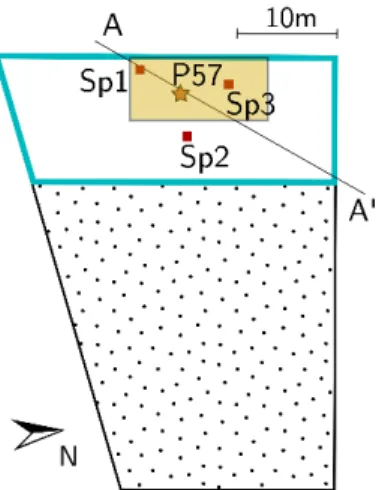
The global efficacy of the sparging was evaluated by monitoring the 1.2-DCB concentrations in P57, in the sparging heads, and in the piezometers located in the direct and lateral downstream direction (see Figure 1). As a whole, the concentration decrease was substantial, but quite heterogeneous, which was unexpected for such a small area. Immediately after the end of the treatment, a significant rebound of the concentrations was observed. The recharge kinetics was measured in the sparging head Sp3 after the end of the last injection cycle, and showed a recovery rate of the order of 50% over four hours. A vertical profile was realized in P57 and revealed 1.2-DCB concentration close to the solubility limit, indicating the presence of free-phase. Such as large value was not found during the search for free-product, and may have resulted here from dissolution/remobilization induced by the sparging. Four months after the end of the treatment, the concentrations had largely increased, and exceeded their initial level. Even though the production of VOCs vapors was exhausted within the first two months, the rebound effect lead to the resurgence of 50 L of free-phase in Sp3, equivalent to 10 L (13 kg) of pure 1.2-DCB after decantation, twice the amount retrieved during the four-months treatment.
Figure 1. 2D-plan of the investigated area. The former solvent tanks location is surrounded in blue, in the western part of the trapeze-shaped perimeter which corresponds the former building boundaries. The general groundwater flow is from A to A’. The star locates the piezometer P57. The red squares locate the sparging heads. The yellow rectangle represents the area where DNAPL was first expected.
In conclusion, this pilot test did not decrease the pollution but released 1.2-DCB that recovery tests did not allow to mobilize. It indicated the presence of contaminated layers that continuously refilled the wellbores. Sparging/venting appeared impractical on a financial and timescale perspective without a proper treatment of these pockets. It was thus decided to opt for another technique, called substitution, whose principle is to drill the areas which are thought to be impacted, and to replace the contaminated materials by an inert substance. For economical reasons, only 155 m2out of the 550 m2of the storage
decide how to spread the 155 m2of soil treatment, complementary investigations were required and to do so, a geophysical campaign was performed.
3. Geophysical survey
3.1. Operations conducted prior to the geophysical survey and preliminary tests
The investigated area was excavated down to a depth of 10 m, i.e. 1 m above the water table (Figure 2), in order to treat the sediments of the unsaturated zone separately and to put them back after the treatment of the saturated zone. Reinforced concrete piles 8 to 15 m deep were lined up along the edges of the pit; in addition, struts were installed to support these walls. The excavation allowed to get closer to the target of interest, i.e. the polluted saturated zone. We took advantage of this to conduct GPR and ERT measurements at the bottom of the pit.
Figure 2. Transverse view of the investigated area. The geophysical campaign was conducted at the bottom of the excavated pit, i.e. 1 m above the water table. The piezometer P57 and the sparging heads Sp1 and Sp3 were removed before the operations; this sketch shows their previous locations.
In addition to these two methods, we conducted spectral IP measurements. We initially planned to use the steel reinforcement inside of two of the concrete piles surrounding the pit as injection electrodes. Unfortunately, a preliminary injection test revealed physical contact between the steel reinforcement located within adjacent piles. We therefore fell back to a more conventional geometry, but our measurements revealed no clear chargeability contrast.
The worksite constraints imposed to collect the data within three days, after the end of the excavation and before the beginning of the substitution. The excavation operations were still ongoing at the start of the geophysical survey.
3.2. Ground Penetrating Radar
3.2.1. GPR data acquisition and processing
GPR data acquisition was twofold. A view of this acquisition is provided in Figure 3a. Since the pit was only partially excavated upon the beginning of the geophysical survey, we were initially limited to the area comprised between y = 0 m and y = 4 m. We therefore acquired two preliminary longitudinal profiles along lines y = 0 m and y = 4 m (Figure 3b), using 500, 250 and 100 MHz antennas. Following these tests, we elected to work with the 250 MHz antenna for the remainder of the GPR survey, as it yielded a good compromise between resolution and penetration depth. We acquired 11 GPR profiles spanning between x= 0 and x = 35 m: the profiles were evenly spaced between y = 0 and y= 4 m, i.e. using a 40 cm spacing between profiles. We acquired 14 additional lines, evenly spaced between y = 4.4 and y = 9.6 m after the pit was further excavated. Since the ground was reworked, we repeated the profile at y= 4 m to verify the consistency between both data subsets. We also acquired 8 transverse GPR profiles between x= 0 and x = 35 m using a coarser spacing of 5 m between profiles (see Figure 3b). In order to complement this dataset, we also acquired 3 longitudinal GPR profiles using the 100 MHz antenna, at y= 0 m, y = 4 m and y = 9 m.
(a) GPR acquisition along a longitudinal profile.
(b) Sketch of the GPR coverage. Grey lines denote the longitudinal profiles, orange lines the transverse profiles. Line AA’ shows the groundwater flow direction.
Figure 3. GPR data acquisition.
The following processing steps were applied to the GPR data:
1. Zero time correction. Knowing the distance between transmitter and receiver antennas and the constant speed of light, we computed the time ta needed by the air wave to travel from the
transmitter to the receiver [31]. We then subtracted it from the time at which the direct air wave was observed, i.e the time of the first event seen in each radar trace. This shift by 28 samples allowed to recover the zero time.
2. Direct Current filtering or dewowing. We removed the low frequency component present in the signal, due to saturation by early arrivals and/or by inductive coupling effects [32]. For each sample
in the trace, we subtracted the arithmetic mean of the amplitudes of the neighbouring samples, computed over a sliding window of 4 ns.
3. Dynamic gain filtering. In order to improve visualization and aid interpretation, we computed the envelope of each trace using Hilbert’s transform; the amplitude of each sample in the trace was then normalized by the amplitude of the envelope at the corresponding time. However, in order to avoid artificially amplifying the amplitude of the late time samples, for which the amplitude of the envelope could be very small, we fixed a threshold Athresat 80 dB below the maximum amplitude
Amaxof the trace. Therefore, if the amplitude of the envelope at a given time was smaller than
Athres= Amax/10, 000, the amplitude of the sample was simply normalized by Athres.
4. Band-pass filtering. Finally, we band-passed the data using a low cutoff frequency of 75 MHz and a high cutoff frequency of 400 MHz.
The processing parameters for data acquired using the 250 MHz antenna are given in the second row in Table 2. For comparison, we also provide in this table the parameters used when working with 100 MHz and 500 MHz antennas.
Table 2. GPR processing parameters.
Antenna frequency n shift Window size Cutoff frequencies 500 MHz 28 samples 2 ns 150–800 MHz 250 MHz 28 samples 4 ns 75–400 MHz
100 MHz 28 samples 10 ns 30–180 MHz
An energy decay gain was also applied to some of the sections: we computed the mean amplitude decay curve for the entire radargram, and then divided the amplitude of each datapoint in each curve by that of the corresponding sample of the decay curve, thus highlighting reflections occurring at late times, that would otherwise remain concealed due to their low amplitudes.
3.2.2. GPR results
The high resolution 500 MHz radargram acquired at y = 4 m reveals a sub-horizontal reflector around 10 ns that could be associated with the water table (WT); this reflector is indicated by the yellow arrows in Figure 4. Considering a uniform velocity of 0.1 m.ns−1, this reflector’s depth is 30 cm, which is consistent with the reported depth of the WT level. The fact that the reflector is discontinuous can be explained by the lateral variations in granulometry, observed while working in the excavated pit. Consistently, the lithological log acquired at borehole P57 (Figure 5) indicates that the first meter below the excavated ground surface consists of greyish sands, gravels and heterogeneous pebbles. Sharp reflectors such as the one highlighted by the left-hand side arrow in Figure 4 could be generated by the WT in coarse material, associated with a narrow capillary fringe; on the other hand, fine material associated with a thicker transition zone would lead to reflectors of smaller amplitudes [33], such as the one indicated by the right-hand side arrow in Figure 4.
In Figure 5 we compare the GPR data with the lithological log of borehole P57. We plot the GPR data between x= 18 m and x = 20 m for sections 13 (y = 4.8 m) and 14 (y = 5.2 m) between which P57 is located. In addition to the WT, highlighted by yellow arrows, several reflectors can be identified. Considering a velocity of 0.1 m.ns−1, two reflectors appear between 1.20 m and 1.60 m, i.e. between
11.20 m and 11.60 m below the former ground level; these could be associated with the transition between the pinkish horizon and the coarse gravel observed about 11 m below the surface, indicated by the topmost dotted line in Figure 5. It is harder to identify a clear reflector associated with the transition between coarse gravel and coarse greyish sand, gravel and pebbles, as highlighted by the second dotted line from the top, around a depth of 12.50 m. This step puts in evidence a reflector around 140 ns in section (a’). One could possibly associate this reflector with the transition from sand to gravel observed around a depth of 17 m in P57, highlighted by the third dotted line in Figure 5.
Figure 4. Close-up view on the 500 MHz radargram acquired at y= 4 m. The yellow arrows indicate the reflector associated with the Water Table (WT).
Figure 5. Correlation between radargrams acquired at y= 4.8 m (a) and y = 5.2 m (b) between x= 18 m and y = 20 m and the lithological log at borehole P57. The same radargrams were represented with a different gain (energy decay) in (a’) and (b’). The yellow arrows designate the WT.
Figure 6. Radar section acquired at y= 4 m using the 250 MHz antenna (upper plot). Results obtained for the 500 MHz antennas are also provided for comparison (lower plot). A mean velocity of 0.1 m/ns was considered here. A dipping reflector is highlighted in yellow in both radargrams: this reflector is associated with a point bar environment.
In the upper plot in Figure 6, we present one of the radargrams obtained using the 250 MHz antenna. For comparison, we also present the same section acquired using a 500 MHz antenna in the lower plot. The same dipping reflector is highlighted in yellow in both radargrams: this reflector could be associated with a point bar environment, formed by lateral accretion along the nearby river bank during meandering channel migration [Duringer, personal communication]. Individual 2D lines can be merged into a 3D cube, allowing to follow the dipping reflectors such as the one highlighted in Figure 6 from one section to the next. These reflectors are observed between 1 m et 4 m below the surface of the excavated area, i.e. between 11 m and 14 m below the initial ground level. For instance, the reflector highlighted in yellow in Figure 6 stretches between z= 1.25 m and z = 2.50 m; its apparent slope is about 16◦. As explained in the legend of Figure 7, due to the orientation of the GPR profiles with respect to the point bar deposits, this apparent slope αappis underestimated with respect to the actual slope. The actual slope α can be
computed from αappand from the angle θ between the dip direction of the reflector and the profile [34]:
α = sin−1 sin(αapp)
cos(θ) !
. (1)
Figure 7. Orientation of a sample GPR section with respect to the former river that led to the deposition of point bar deposits. The former flow of the river was roughly oriented along the B-B’ direction (dark blue line arrow). Note that B-B’ may have changed over time and is not necessarily aligned with the current groundwater flow direction A-A’ (see Figures 1 and 3b). According to the orientation of B-B’, the apparent slope of the reflectors calculated from the radargrams is likely to be underestimated with respect to the actual slope of the point bar deposits.
Considering an apparent slope of 16◦and an angle of 30◦ between the profile and the approximate
flow direction yields a slope value of about 33◦. The tilted reflectors associated with point bar deposits do not provide direct information about the presence of DNAPL in the subsurface. However, their depths are close to those of the PID anomalies identified in P57 at 10 m and 14 m. They signal lithological transitions that could have blocked some DNAPL pools between 6 and 10 m above the bedrock. The log also indicates a transition from coarse gravel to lower permeability sands and pebbles at 12.5 m depth, which supports this scenario.
In the southern part of the imaged area, a reflector that cannot be associated to stratigraphic events can be observed. This antiform reflector is highlighted in red in Figure 6.
3.3. Electrical Resistivity Tomography 3.3.1. ERT data acquisition and processing
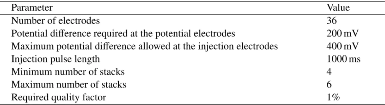
We acquired an ERT profile using a Syscal Pro (IRIS instrument), in Wenner-Schlumberger mode, a configuration moderately sensitive to both horizontal and vertical structures [35]. We opted for this configuration, since we had little prior expectation about the shape of the target. We deployed 36 steel electrodes evenly spaced between x= 0 and x = 35 m, adding saltwater at all electrodes to decrease the ground’s contact resistance. We chose to work with a quality factor of 1%, thus acquiring data until the standard deviation between successive runs fell below 1%, up to a maximum of 6 runs. Our acquisition parameters are detailed in Table 3.
Table 3. ERT acquisition parameters.
Parameter Value
Number of electrodes 36
Potential difference required at the potential electrodes 200 mV Maximum potential difference allowed at the injection electrodes 400 mV
Injection pulse length 1000 ms
Minimum number of stacks 4
Maximum number of stacks 6
Required quality factor 1%
The raw ERT data are presented in Figure 8. The resistivities presented here are apparent resistivities: each data point in the raw section corresponds to the resistivity value that would be associated with an electrically homogeneous and isotropic half-space in order to yield the measured potential difference given the applied current, for the particular electrode spacing corresponding to this data point. In order to obtain true resistivity variations in the subsurface, the data must undergo a process called inversion, detailed in the next section.
3.3.2. ERT data inversion and results
The inversion process consists in simulating synthetic data using a resistivity model and comparing them to the actual data. This procedure is repeated iteratively until a satisfying model is reached, i.e. a model for which the misfit between actual and forward modelled data falls below a given threshold. Several strategies allow to cope with the non-uniqueness of the solution; these are algorithm-dependent but generally involve some kind of regularization such as penalizing sharp resistivity variations in the model [36,37]. The algorithm used here, implemented in the DC2DInvRes program, is based on L-curve analysis [38]: this method allows to find a reasonable trade-off between the data misfit and the model roughness by plotting one against the other for different regularization parameters, yielding a “L-shaped” curve. We use a homogeneous half-space of resistivity ρ= 181 Ω.m as the starting model; this value corresponds to the median of the apparent resistivities. The resulting inverted section, for which a RMS misfit of 2.45% is reached, is presented in Figure 9. Some of the cells in the Southern portion of the section are rejected based on the coverage parameter, defined as the sum of the absolute values of sensitivities over all the measurements. Only cells for which coverage exceed 0.25 are kept in the final section. The poor coverage at greater depths in the Southern part of the profile can be explained by the overburden of relatively higher conductivity in this area, preventing the injected current from flowing deeper into the subsurface.
Figure 9. Inverted ERT section. A RMS misfit of 2.45% is reached after 90 iterations. Only cells for which coverage exceed 0.25 are kept (see text for explanation).
The inverted ERT section shows a global decrease in apparent resistivity with increasing depth. The topmost 50 cm in the Southern part of the profile (highlighted as “a” in Figure 9) show a slightly lower resistivity than the rest of the topmost unit. This increase in resistivity from South to North, ranging from about 500Ω.m to more than 1000 Ω.m, could derive from subtle lithology variations, like the aforementioned differences in granulometry inducing variations in water content. On the other hand, the region comprised between 50 cm and 2.5 m (highlighted as “b” in Figure 9) seems more resistive in the Southern part of the profile than in its Northern half. It is not obvious whether this area of lower resistivity can be associated with a pocket of DNAPL; it is however tempting to correlate this anomaly with the antiform reflector highlighted in red in the GPR section (Figure 6). In this study, the geometry of the pit prevented us from deploying a larger array that could have provided additional insight about this anomaly.
4. Analyses on substitution cuttings
4.1. Cuttings acquisition
The substitution operations started after the completion of the geophysical survey and were spread over several months. The first 87 drillings were mainly performed in the middle of the investigated area, where the pollutant was expected to be trapped following the conclusions of the sparging/venting test, and in the Southern part of the area, where the GPR antiform anomalous reflector was identified. Their purpose was to confirm that the most polluted samples were focused in these areas.
The drill was equipped with a 70 cm diameter auger. When local conditions allowed this auger to reach the marl basement 11 m below the surface, as was the case most of the time, the volume of injected concrete, similar to the volume of withdrawn sediments, was of the order of 4 m3. PID vertical profiles were made by measuring the PID value of the retrieved cuttings around every 3 m, in order to assess the depth of the most impacted layers. Two soil samples were collected from the retrieved sediments, one during the descent of the auger, and another one during its ascent. In total, the first 87 drillings allowed to collect and analyze 172 samples.
Due to the drilling technique, it was not possible to avoid contact between the sediments brought to the surface and the sediments of the upper layers that they crossed. Therefore, the samples collected during the descent of the auger could be vitiated by the layers located above the head of the auger, while the samples collected during the ascent of the auger could be vitiated by all the layers separating the maximum depth reached by the auger from the surface. It is also possible that some mixing occurred. There is thus a significant uncertainty regarding the initial depth of the materials that were analyzed. However, this way to screen the contamination provided a dataset of high spatial density, that would have not been affordable using conventional drilling techniques.
4.2. Comparison with geophysical results
The concentrations measured in the sediments collected through these 87 first drillings are plotted in Figure 10, at the various depths they were taken from. For the samples that were collected during the descent of the auger, these depths are the depths reached by the head of the auger when the sediments emerged at the surface. The concentrations of the samples collected during the ascent of the augers are plotted only if they are greater than the values measured on the sediments retrieved during the descent of the auger at the same locations. By default, they are also plotted as a function of the depth reached by the head of the auger when the sediments emerged at the surface; however, these latter were susceptible to be mixed with materials originating from below. To correct this, the most impacted layer can be estimated thanks to the PID measurements. For a given location, the most impacted layer is likely the layer at which the greatest PID value was recorded. Therefore, for the sediments collected during the ascent of the auger, if the depth reached by the head of the auger when the sediments emerged at the surface is shallower than the depth of maximum PID value, the concentration value is plotted as a function of this depth of maximum PID instead.
The samples depths can be grouped in four layers of ca. 2.5 m, 6 m, 8.5 m and 10.5 m depth. The map of the GPR amplitudes measured at 1.3 m depth is superimposed on the plot corresponding to the closest depth (Figure 10a). The position of the anomalous reflector is located by a black oval. The concentration values are indicated by the colormaps in logarithmic scale. The minimum of the dataset is < 0.10 mg.kg−1(no 1.2-DCB found) and the maximum is 440 mg.kg−1.
10 15 20 25 30 35 5 0 0 5 10 b) depth ≈ 6.0 m 5 0 0 5 10 15 20 25 30 35 10 c) depth ≈ 8.5 m 5 0 0 5 10 15 20 25 30 35 10 d) depth ≈ 10.5 m 5 0 0 5 10 15 20 25 30 35 102 101 100 10-1 10 a) depth ≈ 2.5 m 32788 -32788 0 102 101 100 10-1 102 101 100 10-1 102 101 100 10-1 N
Figure 10. Analysis of the substitution cuttings. The solid circles denote the 1.2-DCB concentrations [mg.kg−1] measured on the cuttings retrieved. The darker the grey level, the
higher the concentration, as indicated by the colorbars next to each map. The initial depths of the cuttings are comprised between 2.0 m and 2.9 m for (a), between 5.3 m and 6.3 m for (b), between 7.9 m and 9.4 m for (c), between 9.8 m and 11.0 m for (d). The map of the GPR amplitudes obtained at 1.3 m depth is superimposed on the plot corresponding to the closest depth (Figure 10a). The black oval locates the GPR anomalous reflector. The small black dots outside of the surveyed area represent the reinforced concrete piles. The blue star denotes the former piezometer P57 and the red squares the former sparging heads.
The measurements obtained from the samples collected around 2.5 m depth are sparse (Figure 10a). At 6 m depth, most of the contaminated materials are focused in the Western edge of the antiform reflector (Figure 10b). This observation can also be made with the deeper samples (Figure 10c,d), whose maximum concentrations are located at the same place. Some high concentration values can be denoted in the central part of the imaged surface. They correspond to samples collected during the ascent of the auger, and may feature the materials lying on the marl basement, in accordance with the suspicion of DNAPL pools blocked on the bedrock. Apart from these isolated spots, the general trend is that the majority of contaminated samples were vertically aligned with the GPR reflector.
The comparison between GPR data and direct concentration measurements did not unveil a correlation between an anomalous reflector and a contaminant pocket, since the high concentration values were measured at depths greater than that of the detected anomaly. However, these analyses confirmed the presence of the seeked pollutant not only in the middle of the investigated area, where it was expected to be found, but also in the Southern part, in the Western half of the black oval locating the GPR anomaly. Based on these elements, the remainder of the substitution operations were conducted so as to focus the 155 m2of treated surface on these areas.
5. Discussion
A multi-method geophysical campaign was conducted at a former dyestuff and pigment formulation plant in order to complement conventional environmental investigations. The initial search for free-phase product and the subsequent sparging-venting tests indeed allowed to infer the presence of a DNAPL source in the survey area but indicated a quite heterogeneous pollutant distribution, thus calling for complementary geophysical measurements.
The depth at which the contaminant was expected to be found, greater than 10 m, initially ruled out GPR as a viable method. GPR is generally not applicable to targets deeper than a few meters, unless boreholes are available. But in order to treat the sediments from the vadose zone, the area of investigation was excavated down to a depth of 10 m, which is 1 m above the water table. This excavation allowed to bypass this limitation, and made GPR applicable. Longitudinal and transverse GPR profiles were conducted at the bottom of the excavated pit using a 250 MHz antenna. These sections allowed to detect the water table and to highlight reflectors corresponding to lithological transitions consistent with the lithological log acquired at a borehole drilled at the center of the area prior to the excavation. GPR also highlighted several 5 to 10 m long dipping reflectors, whose apparent slopes were comprised between 10◦ and 20◦,
interpreted as point bar deposits. Last but not least, GPR unveiled a ∼ 3 m wide antiform reflector in the Southern part of the survey area, at a depth comprised between 1 m and 2 m below the excavated surface. This reflector could not be associated with any known stratigraphic event, but analyses on substitution cuttings confirmed the presence of the pollutant in this part of the survey area. The high concentration values (>100 mg.kg−1) observed there were located at depths greater than 5 m below the excavated level, i.e.
2 to 3 m below the reflector, thus ruling out the hypothesis that this reflector could correspond to a pocket of free-phase contaminant. It was thus hypothesized that this antiform reflector could rather indicate a barrier that upsetted the DNAPL leakage travel. Indeed, the contaminated samples collected near this GPR anomaly were located at the Western edge of this reflector, which might indicate a structure that prevented the lateral migration of the DNAPL in the North-East direction, despite the groundwater movement flowing from South-West to North-East (see Figures 1 and 3b), thus making the DNAPL sink below.
With a resistivity of several hundreds of MΩ.m, the seeked DNAPL was expected to be a resistive target. However ERT indicated a global conductivity increase of the shallow overburden from North to South, thus confirming that the released DNAPL was in a degraded state, as suggested by the presence of bacteria and degradation byproducts.
In turn, no direct detection of DNAPL was made, neither by GPR, nor by ERT. Indeed, while several papers illustrate the efficacy of geophysics to monitor fast DNAPL mass changes during remediation processes [39, 40], the challenge is great when it comes to performing a static imaging of a site impacted by an old pollution, as it was the case here. [41] showed that the GPR amplitudes derive from the quantity of DNAPL forming the pool, and when a DNAPL is released in the environment, its quantity decreases with time as it undergoes dilution and degradation phenomena. [42] monitored the release of a small quantity (50 L) of a mixture of chlorinated solvents in a natural aquifer: after 66 months, they observed that the reflectors amplitude was only about 4% to 9% of the maximum response obtained 1 day after the release. Studies such as the one of [9] proved the ability of ERT to detect at field-scale chlorinated solvents present in free-phase, but not at the state of residual saturation. There is therefore a threshold under which the contaminant quantity remains high enough to induce adverse effects, but too low to generate a detectable contrast of physical property with the host medium.
Because this campaign was performed long after the DNAPL release, GPR and ERT did not allow to image the DNAPL contaminant traces. When dealing with old DNAPL pollution, geophysical imaging should rather be viewed as a means to find preferential paths that the pollutant could have followed. In this example, a correlation could be observed between the presence of stratigraphic events, indicated by GPR, and significant DNAPL concentrations (>100 mg.kg−1) found below, in the Southern and central parts of the survey area. The subsequent substitution operations were thus focused on these locations.
6. Conclusions
This study highlighted the challenges posed by the use of geophysics for remediation purposes on old polluted sites. On the one hand, surface geophysics provides a coverage denser than that of borehole measurements, but on the other hand, its sensitivity to trace contaminants is weak. Resorting to geophysics for the direct detection of contaminant should be done as early as possible throughout the remediation process, in order to take advantage of large contrats between the properties of the free-phase contaminant and that of the surrounding sediments. Various techniques should be applied, but not necessarily at the same time, depending on worksite constraints.
This geophysical survey did not allow to directly image the pollutant, in spite of it being present in large enough quantities to generate a contamination plume with a maximum concentration above the admissible limit. The DNAPL traces in the near surface were too degraded to generate anomalies. However, the antiform reflector highlighted by the GPR in the Southern part of the survey area could correspond to a feature that the pollutant had followed when migrating downward, thus accounting for the pollutants concentrations observed in the substitution cuttings taken below. This part of the survey area was not highlighted by the conventional investigations initially performed. By providing additional information about the soil stratigraphy, this geophysical campaign helped narrow down the remediation process to a surface smaller than the entire excavated area, thus meeting the remediation requirements.
Acknowledgements
The two first authors contributed equally to this work.
The authors would like to thank Myriam Lajaunie for actively taking part in data acquisition and Philippe Duringer for his insightful comments about point bar environments. The authors also would like to thank the companies in charge of the sparging/venting pilot test (Serpol), samples analyses (Eurofins) and substitution (Remea). Special thanks go to Kevin Le Foll and Maxime Gaultier for managing the samples collection during the remediation operations. Finally, the authors would like to thank Jean-Franc¸ois Girard for his thorough reading of this paper.
The authors acknowledge the support of Ramboll France Environment & Health, Institut de Physique du Globe de Strasbourg (CNRS-UMR 7516) and G´eosciences Paris-Saclay (CNRS-UMR 8148).
Conflict of interest
All authors declare no conflicts of interest in this paper.
References
1. Mercer JW, Cohen RM (1990) A review of immiscible fluids in the subsurface: properties, models, characterization and remediation. J Contam Hydrol 6: 107––163.
2. Suthersan S, Horst J, Schnobrich M, et al. (2016) Remediation engineering: design concepts. CRC Press.
3. Nativ R, Adar EM, Becker A (1999) Designing a monitoring network for contaminated ground water in fractured chalk. Groundwater 37: 38––147.
4. Ajo-Franklin JB, Geller JT, Harris JM (2006) A survey of the geophysical properties of chlorinated DNAPLs. J Appl Geophys 59: 177––189.
5. Brewster ML, Annan AP (1994) Ground-penetrating radar monitoring of a controlled DNAPL release: 200 MHz radar. Geophysics 59: 1211–1221.
6. Bano M, Loeffler O, Girard JF (2009) Ground penetrating radar imaging and time-domain modelling of the infiltration of diesel fuel in a sandbox experiment. C R Geosci 341: 846––858.
7. Orlando L, Palladini L (2019) Time-lapse laboratory tests to monitor multiple phases of DNAPL in a porous medium. Near Surf Geophys 17: 55––68.
8. Schneider GW, Greenhouse JP (1992) Geophysical detection of perchloroethylene in a sandy aquifer using resistivity and nuclear logging techniques. In 5th EEGS Symposium on the Application of Geophysics to Engineering and Environmental Problems 1992, 619––628.
9. Newmark RL, Daily WD, Kyle KR, et al. (1998) Monitoring DNAPL pumping using integrated geophysical techniques. J Environ Eng Geophys 3: 7––13.
10. Chambers JE, Wilkinson PB, Wealthall GP, et al. (2010) Hydrogeophysical imaging of deposit heterogeneity and groundwater chemistry changes during DNAPL source zone bioremediation. J Contam Hydrol 118: 43––61.
11. Atekwana EA, Werkema Jr DD, Duris JW, et al. (2004) In-situ apparent conductivity measurements and microbial population distribution at a hydrocarbon-contaminated site. Geophysics 69: 56––63. 12. Binley A, Slater LD, Fukes M, et al. (2005) Relationship between spectral induced polarization and
hydraulic properties of saturated and unsaturated sandstone. Water Resour Res 41. 13. Olhoeft GR (1985) Low-frequency electrical properties. Geophysics 50: 2492––2503.
14. Vanhala H, Soininen H, Kukkonen I (1992) Detecting organic chemical contaminants by spectral-induced polarization method in glacial till environment. Geophysics 57: 1014––1017.
15. Kemna A, R¨akers E, Dresen L (1999) Field applications of complex resistivity tomography. 1999 SEG Annual Meeting.
16. Cardarelli E, Di Filippo G (2009) Electrical resistivity and induced polarization tomography in identifying the plume of chlorinated hydrocarbons in sedimentary formation: a case study in Rho (Milan—Italy). Waste Manage Res 27: 595––602.
17. Cassiani G, Kemna A, Villa A, et al. (2009) Spectral induced polarization for the characterization of free-phase hydrocarbon contamination of sediments with low clay content. Near Surf Geophys 7: 547––562.
18. Orozco AF, Kemna A, Oberd¨orster C, et al. (2012) Delineation of subsurface hydrocarbon contamination at a former hydrogenation plant using spectral induced polarization imaging. J Contam Hydrol 136: 131––144.
19. Johansson S, Fiandaca G, Dahlin T (2015) Influence of non-aqueous phase liquid configuration on induced polarization parameters: Conceptual models applied to a time-domain field case study. Geoexploration 123: 295––309.
20. Blondel A, Schmutz M, Franceschi M, et al. (2014) Temporal evolution of the geoelectrical response on a hydrocarbon contaminated site. J Appl Geophys 103: 161––171.
21. Naudet V, Revil A, Bottero JY, et al. (2003) Relationship between self-potential (SP) signals and redox conditions in contaminated groundwater. Geophys Res Lett 30.
22. Minsley BJ, Sogade J, Morgan FD (2007) Three-dimensional self-potential inversion for subsurface DNAPL contaminant detection at the Savannah River Site, South Carolina. Water Resour Res 43. 23. Temples TJ, Waddell MG, Domoracki WJ, et al. (2001) Noninvasive determination of the location
and distribution of DNAPL using advanced seismic reflection techniques. Groundwater 39: 465––474.
24. Waddell MG, Domoracki WJ, Temples TJ (2001) Use of seismic reflection amplitude versus offset (AVO) techniques to image dense nonaqueous phase liquids (DNAPL). In 14th EEGS Symposium on the Application of Geophysics to Engineering and Environmental Problems.
25. Vaudelet P, Schmutz M, Pessel M, et al. (2011) Mapping of contaminant plumes with geoelectrical methods. A case study in urban context. J Appl Geophys 75: 738––751.
26. Sparrenbom CJ, Åkesson S, Johansson S, et al. (2017) Investigation of chlorinated solvent pollution with resistivity and induced polarization. Sci Total Environ 575: 767––778.
27. Kueper BH, Stroo HF, Vogel CM, et al. (2014) Chlorinated solvent source zone remediation. Springer.
28. Davis JL, Annan AP (1989) Ground-penetrating radar for high-resolution mapping of soil and rock stratigraphy. Geophys Prospect 37: 531––551.
29. Lucius JE, Olhoeft GR, Hill PL, et al. (1992) Properties and hazards of 108 selected substances—1992 edition. US Geological Survey Open-File Report, 92: 527––554.
30. Pankow JF, Cherry JA (1996) Dense chlorinated solvents and other DNAPLs in groundwater: History, behavior, and remediation. Waterloo Press.
31. Kirsch R (2008) Groundwater Geophysics: A Tool for Hydrogeology. Springer Verlag GmbH. 32. Jol HM (2008) Ground penetrating radar theory and applications. Elsevier.
33. Bano M (2006) Effects of the transition zone above a water table on the reflection of GPR waves. Geophys Res Lett 33: L13309.
34. Yilmaz O (1987) Seismic Data Processing. Society of Exploration Geophysicists.
35. Loke MH (2000) Electrical imaging surveys for environmental and engineering studies–A practical guide to 2-D and 3-D surveys.
36. Loke MH, Barker RD (1996) Rapid least-squares inversion of apparent resistivity pseudosections using a quasi-Newton method. Geophys Prospect 44: 131––152.
37. Sharma S, Verma GK (2015) Inversion of electrical resistivity data: a review. Int J Environ Chem Ecol Geol Geophys Eng 9: 400––406.
38. G¨unther T, R¨ucker C, Spitzer K (2006) Three-dimensional modelling and inversion of DC resistivity data incorporating topography-—II. Inversion. Geophy J Int 166: 506––517.
39. Daily W, Ramirez A (1995) Electrical resistance tomography during in-situ trichloroethylene remediation at the Savannah River Site. J Appl Geophys 33: 239––249.
40. Power C, Gerhard JI, Karaoulis M, et al. (2014) Evaluating four-dimensional time-lapse electrical resistivity tomography for monitoring DNAPL source zone remediation. J Contam Hydrol 162: 27––46.
41. Brewster ML, Annan AP, Greenhouse JP, et al. (1995) Observed migration of a controlled DNAPL release by geophysical methods. Groundwater 33: 977––987.
42. Hwang YK, Endres AL, Piggott SD, et al. (2008) Long-term ground penetrating radar monitoring of a small volume DNAPL release in a natural groundwater flow field. J Contam Hydrol 97: 1––12.
© 2021 the Author(s), licensee AIMS Press. This is an open access article distributed under the terms of the Creative Commons Attribution License (http://creativecommons.org/licenses/by/4.0)
![Table 1. Properties of 1.2-dichlorobenzene at a temperature of 25 ◦ C, after [29].](https://thumb-eu.123doks.com/thumbv2/123doknet/14790785.601303/5.892.110.799.242.406/table-properties-dichlorobenzene-temperature-c.webp)