Contribution of environmental factors to crop yield variation in the US

Contribution of Environmental Factors to Crop Yield

Variation in the US

By

Gabriel T. Brien

B.S., Civil Engineering

North Dakota State University

Submitted to the Department of Civil and Environmental Engineering in Partial Fulfillment of the Requirements for the Degree of

Master of Engineering in Civil and Environmental Engineering

at the

Massachusetts Institute of Technology

( 2017 Gabriel T. Brien. All Rights Reserved.

The author hereby grants MIT permission to reproduce and distribute publicly, paper and electronic copies this thesis documenor in part any medium now known or hereafter created

Signature of Author:

S ignature redacted

Department of Civil and Environment

Certified by:

Signature re

Gabriel Brien al Engineering

dacted

Dennis B. McLaughlin H.M. King Bhumibol Professor of Water Resources Management

Accepted by:

Signature redacted

MIASSAH SL INSTITUTE OF TECHNOLOGY

JUN 14 2017

LIBRARIES

Professor of Civil and Environmental Engineering Chair, Graduate Program Committee

Contribution of Environmental Factors to Crop Yield

Variation in the US

By Gabriel Brien

Submitted to the

Department of Civil and Environmental Engineering

on May 17th, 2017, in partial fulfillment of the requirements for the degree of

Master of Engineering in Civil and Environmental Engineering

Abstract

The magnitude of crop production per unit area has increased in the US in the last 50 years due to the green revolution (Femandez-Comejo, 2004). Yet, even with these increases, there is still variability in crop yield that is present in modem, intensive agricultural systems (Porter and Semenov, 2005). This variability has a negative effect on food security which depends on a minimum amount of food being available at a given point in time. By definition, food cannot be secure unless it is guaranteed to a certain level (Maxwell, 1996). Hence, an understanding of crop yield variability is essential to the question of food security.

Using a linear mixed effects analysis for a particular US state and a particular crop, environmental factors that affect variability were shown, in both irrigated and rainfed crop situations to explain over 80% of yield variance. The variance was linked to two major factors: daily air temperature and soil moisture. For rainfed yield, temperature effects explained 40% of the yield variance while soil moisture explained 43% of yield variance. For irrigated yield temperature effects explained 87% of the yield variance.

The results suggest that yield variance occurs from variation in the season averages, and in specific points in the growing season, for the major factors highlighted. This assessment is confirmed by moisture and temperature sensitivity characteristics of the crop in question. It is shown by exploratory, time series, and spatial analysis that low yield observations have contrasts in growing season conditions both during key crop reproduction periods and over the entire season. Herein it is argued that variation in temperature effects and moisture have the highest effect on crop yield particularly when they occur during the reproductive phase of the plant.

Thesis Supervisor: Dennis B. McLaughlin

Acknowledgements

I would like to thank everyone who helped me put this thesis together. I would like to thank God and the Blessed Mother for their help and for their assistance to proceed with every day. I would like to thank my parents and siblings for giving me the start and experiences to pursue the opportunities set before me.

I would also like to all those from the Parson's lab that have helped make my learning journey a special one. Particularly my advisor, Dr. McLaughlin, for all his help in critiquing this thesis, direction in research, and all the support in between. Also, I would like to particularly thank the Ph.D students of the McLaughlin group Anjuli, Reetik, and most of all Tiziana who supplied not only helpful input, but also great conversation throughout my time here.

Finally, I would like to thank my fellow M.Eng students Sami and Jon for their support, conversation, and help in pursuing the different challenges presented over the course of year.

Table of Contents

Contribution of Environmental Factors to Crop Yield Variation in the US ... 1

Contribution of Environmental Factors to Crop Yield Variation in the US... 2

A b stract ... 2 Acknowledgem ents... 3 Table of Contents... 4 List of Figures ... 7 List of Tables ... 11 Section 1... 12 Introduction... 12 1.1 M otivation ... 12

1.2 Research Question and Objectives ... 15

1.3 Literature Review ... 15

1.3.1 Studying Yield Variation Via Environm ental Variation... 15

1.3.2 Studying Yield Variation Via Management and Typology Variation ... 16

1.3.3 M oving Forward... 16

1.3.4 In Brief ... 17

S ectio n 2 ... 18

Data and Data Applications ... 18

2.1 Source, Basis, and Reasons for Use of Chosen D ata... 18

2.1.1 Yield, M anagem ent, and Typology ... 18

2.1.2 Environm ental... 19

2.2 Initial Processing and Organization of the Selected Data... 20

2.2.1 Yield, M anagem ent, and Typology ... 20

2.2.2 Environm ental... 21

2.3 Data Applications... 21

2.3.1 Exploratory Analysis ... 21

2.3.2 Linear M ixed Affects Analysis ... 23

2.3.2.1 Linear M ixed Effect M odel Application... 23

2.3.2.2 Basic Linear M ixed Effects M odel Equation... 23

2.3.2.4 Linear M ixed Effects: Assum ptions ... 27

2.3.2.5 Understanding LM E Input and Output ... 27

2.3.3 Spatial and Tem poral Variation ... 28

Section 3... 30

Exploratory Analysis ... 30

3.1 Exploring Data... 30

3.1.1 Yield and Typology ... 30

3.1.2 Yield and Environm ental Variables... 34

3.1.3 Yield and Phenology... 37

Section 4... 40

Linear M ixed Effects Analysis ... 40

4.1 M ethods and M odel... 40

4.1.1 Rainfed LM E ... 40

4.1.2 Irrigated LM E ... 43

4.1.3 Corroboration of Rainfed and Irrigated Results... 47

Section 5... 51

Spatial and Temporal Variation ... 51

5.1 A Specific Case of Variation ... 51

5.1.1 Rainfed County Com parison... 51

5.1.1.1 Rainfed, Tim e Series Variation...52

5.1.1.2 Rainfed, Spatial Variation... 53

High Yield...54

Low Yield ... 56

5.1.2 Irrigated County Com parison ... 57

5.1.2.1 Irrigated, Tim e Series Variation ... 57

5.1.2.2 Irrigated, Spatial Variation... 59

High Yield... 60 Low Yield ... 62 Section 6... 64 Discussion ... 64 6.1 Discussion of Results... 64 Section 7... 66

7.1 Conclusions ... 66

7.2 Contributions ... 67

7.3 Closing ... 67

List of Figures

Figure 1 - Rainfed Corn Yield for 4 US states over Years 2000-2015. Mean taken over all states and all years, 2000-2015. (National Agricultural Statistical Service 2017) ... 13 Figure 2 - Comparison of county rainfed corn yields for the State of Nebraska for the years

2000-2015. Each line represents a set of yields for a county wherein the thick portion of the error bar contains the m ajority of the yield range... 14

Figure 3 - Comparison of county irrigated corn yields for the State of Nebraska for the years 2000-2015. Each line represents a set of yields wherein the thick portion of the error bar contains the majority of the yield range, and the dots represent the minority outliers ... 14 Figure 4 - Kernel Density Plots for 3 Major US Crops for 2000-2015... 33 Figure 5 - Relative Soil Water Holding Capacity for Nebraska Soils. (Wilhelmi and Wilhite,

2002) Areas with smallest capacities are primarily sandy soils. ... 34 Figure 6 - Average mean, daily air temperature for growing season in Nebraska from 2000-2015 ... 3 5

Figure 7 - Average Soil Moisture distribution temperature for growing season in Nebraska from 2 0 0 0 -2 0 15 ... 35 Figure 8 - Average Rainfed Corn Yield in Nebraska from 2000 - 2015 ... 36

Figure 9 - Average Irrigated Corn Yield for Nebraska from 2000-2015 ... 36 Figure 10 -Typical corn water over course of growing season (Kranz et al. 2008). (Note:

Number of days from day 0 to harvest can be shorter for different corn varieties)... 38 Figure 11 - Corn Yield Reduction in Percentage of final yield per day of stress (Shaw and

Figure 12 - Optimal temperature range for corn. (Neild and Newman, 1990) (For reference, 95 F

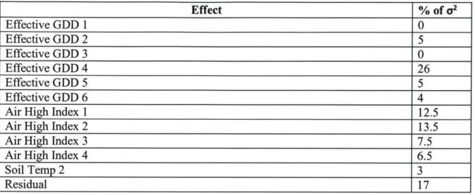
is ro u gh ly 35 C ) ... 39 Figure 13 - The percentage of rainfed yield variance explained by each factor input into the base L M E m o d el... 4 2

Figure 14 - The percentage of irrigated yield variance explained by each factor input into the

b ase L M E m odel ... 4 5

Figure 15 - Relationship between rainfed yield and the average high temperature over growing season for yield location (Note: Values are in columns due to fact that rounded data used from LME analysis which incorporated a finite number of X values)... 47 Figure 16 - Relationship for best and worst rainfed yields and the average high growing season temperature for the yield location (Note: Values are in columns due to fact that rounded data used from LME analysis which incorporated a finite number of X values)... 48 Figure 17 -Relationship between irrigated yield and the average daily max temperature

difference over growing season for yield location (Note: Values are in columns due to fact that rounded data used from LME analysis which incorporated a finite number of X values) ... 49 Figure 18 -Relationship between the best and worst irrigated yields and the average daily high temperature over growing season for a yield location (Note: Values are in columns due to fact that rounded data used from LME analysis which incorporated a finite number of X values) .... 49

Figure 19 -Comparison of rainfed yield from Nebraska counties for the years 2002 and 2009 resp ectiv ely ... 5 2

Figure 20 - State average soil moisture for each day of the Nebraska growing season for years of 2002, 2009, and 2000-2015 average with time of peak, crop water use superimposed ... 52

Figure 21 -State average, daily, high, temperature for each day of Nebraska growing season for

years of 2002, 2009, and 2000-2015 average ... 53

Figure 22 -Rainfed corn yield for the state of Nebraska by county in 2009... 54

Figure 23 -Average Daily High Temperature by County for State of Nebraska in 2009 relative to m e an ... 5 5 Figure 24 -Average Daily Soil Moisture by County for State of Nebraska in 2009 relative to

m e an ... 5 5 Figure 25 -Rainfed corn yield for the state of Nebraska by county in 2012... 56 Figure 26 -Average Daily High Temperature by County for State of Nebraska in 2012 relative

to th e m ean ... 5 6 Figure 27 - Average Daily Soil Moisture by County for State of Nebraska in 2009 Relative to

th e M ean ... 5 7 Figure 28 -Comparison of irrigated yield from Nebraska counties for the years 2002 and 2009 resp ectively ... 5 8 Figure 29 -State average, high, temperature for each day of the Nebraska growing season for

years of 2002, 2009, and 2000-2015 average ... 58 Figure 30 - State average, temperature difference for between the daily high and low for each day of the Nebraska growing season for years 2002, 2009, and 2000-2015 state average ... 59 Figure 31 - Irrigated corn yield for the state of Nebraska by county in 2009 ... 60 Figure 32 -Average Daily High Temperature by County for State of Nebraska in 2009 relative to th e m ean ... 6 1 Figure 33 - Nebraska State average, daily, temperature difference between the daily high and low , over grow ing season for 2009... 61

Figure 34 - Irrigated Corn yield for the state of Nebraska by county in 2002 ... 62 Figure 35 -Average Daily High Temperature by County for State of Nebraska in 2002 relative to th e m ean ... 6 2

Figure 36 -Nebraska State average, daily, temperature difference between the daily high and low, over growing season for 2002... 63

List of Tables

Table 1 - Typical W orld Yields (FAO 2017) ... 12

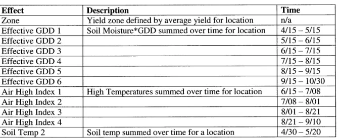
Table 2 - List of regressed typology variables regressed against yield with range of R-square. 31 Table 3 - Crops and corresponding regression variables that had the highest R-square value w hen regressed against the crop ... 32 Table 4 - Definition of variables used for LME model for crop yield ... 41 Table 5 - Variables used in LME model with corresponding amount of yield variance explained by each variable in base m odel... 42 Table 6 - Likelihood ratio test results as compared with initial LME model. Variables were progressively removed such that the final run had only two variables remaining from the initial model. Information expressed is equivalent to: Effect on yield due to variables removed

expressed by A residual(i),

x

Table 8 -Variables used in LME model with corresponding amount of yield variance explained b y each v ariab le ... 4 5 Table 9 -Likelihood ratio test results as compared with initial LME model. Variables were progressively removed such that the final run had only two variables remaining from the initial model. Information expressed is equivalent to: Effect on yield due to variables removed

Section 1

Introduction

1.1 Motivation

The magnitude of crop production per unit area has increased in the US in the last 50 years due to the green revolution (Fernandez-Cornejo, 2004). Yet, even with these increases, there is still variability in crop yield that is present in modem, intensive agricultural systems (Porter and Semenov, 2005). This variability has a negative effect on food security which depends on a minimum amount of food being available at a given point in time. By definition, food cannot be secure unless it is guaranteed to a certain level (Maxwell, 1996). Hence, an understanding of crop yield variability is essential to the question of food security.

Abrupt shifts in the amount of food present can have large impacts on populations, particularly in developing countries. These are countries that may live on a year to year basis with food since there can be a lack of money to import. Historically, this can be seen in situations such as the 2011 drought in the Horn of Africa where sub-average rains affected crop yields and contributed to detrimental population effects (Guha-Sapir et al. 2012).

In developing world countries, there is a push to help populations grow more food so that they feed more of their populations or potentially export food for a profit (Toenniessen et al., 2008). This push is made with the perception that these countries should follow in the developed world model of food production, so that they can annually produce as much food as they need. As an example, average yields for various countries are shown in table 1.

Table 1 - Typical World Yields (FAO 2017)

Country 2008-10 Avg. Corn Country 2008-10 Avg. Corn

Yield (T/Ha) Yield (T/Ha)

Tanzania 1.3 China 5.4

Ghana 1.8 Australia 5.7

Nigeria 2 Argentina 6.6

Ethiopia 2.3 Canada 9.1

The data in table 1 supports emulation of the US and others' model for crops due to the increased

magnitude of production. Yet that idea makes the critical assumption that variations from the

mean yield are minimal enough that food security will still be attained. Yet for areas of US

production, this is not the case. In the US, if given locations are observed for a period, variations

of over

50%

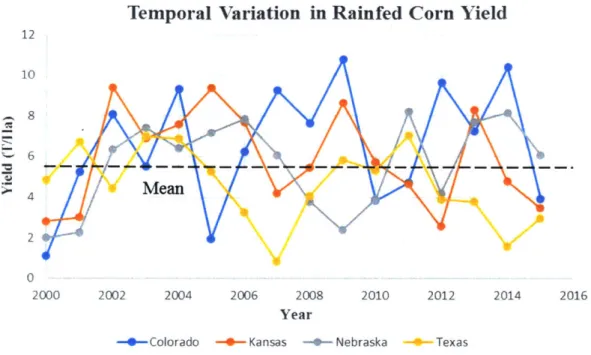
of the mean yield are observed. This is exemplified in figure 1.

Temporal Variation in Rainfed Corn Yield

-- Colorado -- Kansas -0- Nebraska - Texas

Figure 1 - Rainfed Corn Yield for 4 US states over Years 2000-2015. Mean taken over all states and all years, 2000-2015. (National Agricultural Statistical Service 2017)

Since this is a conglomerate of states the mean is reasonable. But if instead, each state relied

upon its own corn crop as its primary staple in a given year, then a state that was doing fine in

the year 2002 with a yield of 7 T/Ha would potentially be starving in 2008 with a yield of 2.5

T/Ha.

This sort of variability is also within states of a given region and can occur in both rainfed and

irrigated crop systems. If a single area is observed, both spatial and temporal variability can be

seen. For example, in Nebraska, if the state corn crop is observed, difference in yield for a given

year or location can exceed 25% of the average yield in irrigated corn, and exceed 50% of

average yield for rainfed corn. This is shown in figures 2 and 3.

Comparison of County Level Rainfed ( orn Yields for Ncbratksa from 2000-2015 16 10 8 6

I

I I

i1

I

II

I:

Figure 2 - Comparison of county rainfed corn yields for the State of Nebraska for the years

2000-2015. Each line represents a set ofyields for a county wherein the thick portion of the

error bar contains the majority of the yield range

Comparison of County Level Irrigated Corn Yields for Nebraska from 2000-2015

16 14

v

Figure 3 - Comparison of county irrigated corn yields for the State of Nebraska for the years 2000-2015. Each line represents a set ofyields wherein the thick portion of the error bar

contains the majority of the yield range, and the dots represent the minority outliers

1.2 Research Question and Objectives

Why is there a state yield for Colorado of 2 T/Ha in 2005 and 11 T/Ha in 2009 or why is there a county in Nebraska (County 37) with a rainfed yield range from 3 T/Ha to 12 T/Ha? The overall question that this thesis is setting out to answer is why large temporal and spatial variations exist for crop yield in the US. This thesis is seeking key variables that have the largest effect on yield, so that they can be explored and quantified.

The key yield variables being considered are broken up into two categories: environmental and management/typological. Environmental variables are anything that is out of the control of the farmer raising the crop: precipitation, temperature and related. Management/typological

variables consist of things that are at least partially in control of the famer raising the crop such as: farm size, machinery, tillage techniques, and fertilizer use. Typology variables are

distinguished as being those related to economic status (i.e. -farm size) and management is primarily crop management (i.e. - tillage techniques)

Given the question, there are two primary objectives for this thesis: 1) highlight the

environmental, farm management, and farm typology variables that have the largest effect on yield for a given crop; 2) highlight the nature of interaction of variables with the crop and the subsequent effect on yield.

The goal is to begin to understand the true nature of what affects crop yields, and thus contribute to the overall understanding of how the issue of variability should be approached. For in

understanding variability, systems that minimize variability can be designed, and efforts that seek to build food security can be further optimized to deal with real-world conditions.

1.3 Literature Review

1.3.1 Studying Yield Variation Via Environmental Variation

There have been numerous papers that have sought to bring attention to the effect of key

environmental variables on yield. Ray et al. (2015), in studying climate through global level data sets, at the monthly temporal scale, argued that temperature, precipitation and their interactions can be linked to a third of yield variation globally. This result was further argued by Iizumi and Ramankutty (2016) who emphasized that large temperature ranges were the single most

important factor in explaining yield variation, even more so than a lack of available moisture. lizumi and Ramankutty also used a higher number of climate variables and at a daily instead of monthly temporal resolution.

For the US, research has shown the effect not only of temperature but also of variation during particular months. Urban et al. (2012) showed that temperature variation during mid-summer

months particularly, lead to yield variation for maize; this corroborates well with Schlenker and Roberts (2009) who showed non-linear response of crop yield to temperature. On a similar vein, Grassini et al. (2014) showed that variation of precipitation during these same months can have a detrimental effect on soybeans complementing Suyker and Verma (2009) who showed the peak water use of soybeans as being during those months.

1.3.2 Studying Yield Variation Via Management and Typology

Variation

Smith et al. (2007) suggested that there was variation depending on management but that it is only seen in differences in organic vs non-organic. Kravchenko et al. (2004) argued for variation that was partially dependent on management, though results were not distinct. More literature was surveyed, but many of the results were conflicting.

Cornia (1985), Schurle (1996), Cabras et al. (2010), and Reidsma et al. (2007) presented various links of farm typology to yield variability, while commenting also on links to climate variation as well. The effect magnitudes differed in each study which indicates that there are effects that depend on location and scale of the study presented that can begin to affect the context of observed changes. Furthermore, it allows insight into the fact there are varying degrees of response towards certain factors in given areas, and unlike environmental variables that can be isolated, often the variables that contribute to the effects of typology and management on yield variation are difficult to define.

1.3.3 Moving Forward

In this study, the primary aim was to investigate yield variability from both a climatic

perspective, and from a typological perspective so that relative importance could be assigned to each. This exploration differs from previous efforts in that it does not assume initially the variables that have the largest effect on yield. Using exploratory analysis, and some linear mixed effects, the variables are screened to understand which has the largest effect. This is done to emphasize a data driven approach that is not skewed by assumption.

The intent is not to minimize the role of any given variables, but rather draw attention to those of highest importance so that in future analysis, those who expand on this work may be allowed to choose a path that has been already categorized.

1.3.4 In Brief

This thesis strives to answer the question of yield variability by first, in section 2, giving a summary of the data used and an overview of how it was initially applied to the problem at hand. Next, exploratory analysis which gives an understanding of which variables should be pursued is discussed in section 3. In section 4, the use of linear mixed effects analysis to further delineate importance of certain variables in the context of a single US state, for a single crop is presented. In section 5, a time series analysis is shown that highlights the elements of importance during a given growing season along with contrasting differing yield conditions. Finally, in section 6, the results from sections 3-5 are discussed which leads into the conclusion of the results and

Section 2

Data and Data Applications

2.1 Source, Basis, and Reasons for Use of Chosen Data

The data used for this analysis are readily available on open internet sources. Initially, in consideration of what would provide insight for work with yield variability, the largest amount of quality data possible was desired. To ensure the highest quality data available at the highest resolution, the US was chosen as the area of analysis. No other country surveyed had similar levels of volume and resolution for all desired data sets. To eliminate issues of comparing

dissimilar crop types, only the data from years 2000-2015 was considered for the questions explored. Also, only areas that distinguished irrigated from non-irrigated crop production were used. It is important to note that this does not encapsulate the entire US and may leave out large production areas.

2.1.1 Yield, Management, and Typology

For crop yield, management and typology variables, the US has data that is available from the National Agriculture Statistical Service (NASS) which is a sub-branch of the USDA. They are

the only source of this type of comprehensive data in the US, and to the knowledge of the author, are the only data to this width in the world that is easily accessible. NASS was the only source of all data used in this thesis for yield, management, and farm typology information (National Agricultural Statistical Service 2017).

There is data that is collected by individual US states for specific areas, in terms of yield and other related information, but is more difficult to obtain. Therefore, while these data were investigated, in the interest of time, they were not utilized.

NASS collects agriculture data in one of two ways: through the US agricultural census

(conducted nationally, every 5 years) and through surveys that are sent to producers. Data from both the Census and from the surveys were used for this thesis.

For the Census on Agriculture, in every census year since 1997, NASS has published on their website a range of statistics relating to categories that include 1) Animals and Products, 2) Crops, 3) Demographics, 4) Economics, 5) Environmental. Thus, all information from the Census

relates to one of the 5 categories and is then organized in geographic regions for the county, state, regional, and national levels. The county level data represents an aggregate count of all producers in that county, and likewise for state, regional, and national levels. Thus, for statistics like crop yield, a county measure represents an average of producers in a county. For a number like total crop production the number for a county represents a sum.

For data collected by surveys, producers within a given set of states or some other region are selected at random. Unlike the Census on Agriculture, the survey is not comprehensive, thus this means that all information for an area in the survey is pieced together from random samples within the area. However, it is collected every year for the same sets of observations. Using statistical methods, the information is up-scaled to the entire geographical boundary of interest. The producers are asked to report data either via online forms, paper forms, or by a phone. The surveys collect less information than the Census since they are singling out aspects of interest on a yearly basis (such as yield), which often means that there is not information

available for some of sub-categories contained within the 5 primary ones listed for the Census or it is not at as fine a spatial resolution. This is the case for information related particularly to management and typology data, which is often presented at the county level for Census years and at the state level for survey years. This is simply because the surveys do not take a large enough

sample size from each county to acceptably minimize the data's coefficient of variation.

2.1.2 Environmental

The environmental data used were obtained from two sources. Data from other sources were considered, but the amount of either spatial or temporal coverage was not suitable for the

application.

One data set used was from the PRISM model published by Oregon State which distributes gridded temperature and precipitation in a 30 arc-second (- 800 m) gridded format (PRISM. 2004). Their data for maximum, minimum, and mean daily temperature, along with precipitation, were used in the analysis.

The data generated by the PRISM model are created through a cell-by-cell regression that is weighted by physical characteristics, including elevation and location relative to other primary physical features of a cell and the presence of an observation within the cell. The temperature grids are integrated with roughly 10,000 observation points, and the precipitation with roughly 13,000 observation points (Daly et al., 2008).

The second dataset used was the NASA NCALDAS (Jasinki et al.) which is based on the NLDAS-2 NASA model. Values of soil moisture and soil temperature for the top 10 cm of soil were used. These were generated by the NOAH land surface model (LSM). Using various data from different sources, the LSM generates a set of parameters of interest in a gridded format at the .125 degree (- 14 km) resolution (Mitchell et al. 2004). The NCALDAS uses observations of

parameters including precipitation and temperature to drive a land surface model (LSM) that integrates an entire collection of climate variables that are used to provide a complete view of the US climate system. NCALDAS was the only dataset found that rendered the desired temporal resolution of 1 day, and the portion of time desired, 2000-2016.

2.2

Initial Processing and Organization of the Selected Data

The goal for this thesis, was to use a data driven analysis. Data collected were processed and organized so that as much of the heterogeneity within the data could be preserved as possible. Unless otherwise noted, all data used was normalized over a mean. Thus, allowing comparisons to be made so that dimensionality did not have to be assigned.

2.2.1 Yield, Management, and Typology

The NASS data for typology, management and yield was broken up into two categories for processing: census years and survey years.

The data used from the agricultural census comprised of 3 years, 2002, 2007, and 2012, at the county level. The county level data rendered yield for every crop grown in the county, along with typological and management data for the county.

For the census, since the typological and management information for a given year was not exactly the same, due to the evolution of the census structure with time, data that was not common to all three census years was rejected.

The typological and management data were also filtered via common logic to eliminate variables that would not be relevant in terms of production. The data were tabulated in a form that was indexed first by year, subsequently by county, finally by attribute. Every year of interest was assigned a set of counties, where each county was given a yield, and a set of

typological/management attributes.

The survey data available spanned yield, typology and management for all years between 2000-2015 not included in the census. Due to smaller sample sizes, the survey data for typology and management variables of interest were typically only available at the state level. However, since the emphasis of the survey data is yield, it is available at the county level. Surveys were not always taken in the same state for a given variable, thus typological/management data were not available consistently.

Hence, for the survey data, the available typological/management data at the state level, and the county level were ignored and only the yield data from the county level were used. The data

were subsequently organized in a table wherein yields for crops were indexed first by year, then by crop, and finally by county.

2.2.2

Environmental

To create a set of environmental variables that could be used with both the census and survey data, environmental data were aggregated to the county level. In its raw form, the data were obtained in gridded format at a daily temporal resolution. From there, it was aggregated over the counties of interest to establish an average for every county on every day. At that point, the data were tabulated, and ranges of interest were selected for different analyses. The tabulated data were indexed by year, county, and finally by day.

2.3

Data Applications

Once the data were obtained, they were analyzed with three separate methods to understand the potential links of different factors to yield variability. The exploratory analysis was implemented to get a basic understanding of potential links to variability might be, the linear mixed affects to narrow down the relative importance of variables, while the time series and spatial analysis was

used to corroborate the mixed affects and further understand the data.

2.3.1 Exploratory Analysis

For this portion, minimal processing of the data was done, so that the maximum amount of heterogeneity would be preserved. Also, only US census data were used, so that environmental, yield, typological, and management variables could be matched.

This portion of the analysis was introductory so that ideas for further analysis could be highlighted. Probability distribution plots were used to understand the structure of the data of interest for yield, typology and environmental variables. The crop yields used included Corn, Wheat (Winter and Spring), Sorghum, Rice, and Soybeans for all denoted irrigated and rainfed areas in the US. The environmental data in question were first selected for every year of interest after which it was subset and averaged over the growing season for the US. In this thesis the growing season is defined as being from April 1 5th to October 3 0th.

Management, environmental, and typological variables, were regressed against yields for the crops of interest. For example, the variable "Income / Farm" for each county and each year was plotted against crop yields for those counties in those years. Prior to regression, all variables were normalized over the mean so that a uniform scale could be used as a comparison.

The data applied within the exploratory analysis took the following form for scatter plots where all i's and j's were graphed on single graph for given crop yield - variable combination. This was done for both crops over the entire US.

Mi, & Ti, & Etjy = X Coordinate

yi,j = Y Coordinate

Where:

Yi, j= Yield for year i in county j M i, j= Management in year i in county j

E p, i, j= Environmental variable, with growing season average pi,

county j

in year i, in

The maps over the entire US the exploratory analysis were made by mapping the following variables:

For each county

j:

Average yield for each county =( i_(yi,))

Average level of each environmental variable = (!X

(

Where:

E a, b, i,j = Environmental variable a, for day b, for year i, and county j.

In the progression of the exploratory analysis it was desired that spatial variability isolated. To do this, the data were pared down such that the state of Nebraska corn crop was selected. Nebraska was selected partially for its environmental qualities, and it spatial uniformity with respect to corn wherein over 60 (out of 93) Nebraska counties have on average 50% or more of their active cropland planted to corn. For Nebraska, primarily mapping was done to link spatial patterns in yield to environmental variables and physical features.

2.3.2 Linear Mixed Affects Analysis

This portion of the analysis was set up to take variables of highlighted importance from the exploratory analysis and to investigate them further.

For the linear mixed affects (LME), survey yields and environmental data from the years 2000-2015 were used. Farm typology and management data were not included since they did not span the years desired, and based on exploratory analysis, did not appear to have a substantial effect

on yield.

In the context of the LME, all models were applied to strictly to corn in the state of Nebraska as an extension of the latter portion of the exploratory analysis. This was done to simplify the analysis, thereby eliminating sources of variability in growing conditions that would be

introduced by large spatial scales. Corn was selected due to its importance as both an economic driver and a staple. Though not initially considered, corn's sensitivity to certain environmental

variables proved useful in amplifying the changes observed to given levels of environmental perturbation.

2.3.2.1 Linear Mixed Effect Model Application

The LME model was applied in two basic cases: rainfed corn and irrigated corn. By

consideration of the physical differences between these two systems, it was assumed that effects on yield variability would be different for each. Thus, environmental variables were inserted into each model based on that assumption and adjusted accordingly.

The basic process that the LME model followed was to group each yield into multiple sets of subset sand thus assign fixed or random effect to each yield based on membership to given subsets. The model was then optimized to find the set of random effects that had the most fitness in minimizing the variance of a set of linear equations for the model against the observed data.

2.3.2.2 Basic Linear Mixed Effects Model Equation

Linear mixed effects (LME) is method of linear regression that works by using a linear regression model with the addition of coefficients that act to modify the model based on

membership to a specific combination of grouped values. The equation as applied in this thesis, and as per Bates (2009), can be described in its basic form as:

Where:

Y = Vector of observed crop yields

X = Known design matrix relating fixed effects to yield Z = Known design matrix relating random effects to yield

P

The unknown vectors were the elements that were varied within the model to create an optimal fit. The vector of observed crop yields and design matrices that were input into the model consisted of the following:

yij = Y = Yield Vector

Zoney = X = Design matrix relating fixed effects to yield

Ea,c,i,j = Z = Design matrix relating random effects to yield

= Eb=bx(Ea.b aiI)

Where:

Zone y = Yield zone y

E a, c, i, j= Environmental variable a over interval c, in year i, for county

j

Thus, each yield from the yield vector was matched with variables from each specific year and county and a corresponding zone.

In the model, the term effect is defined a coefficient that changes the output. These effects

The model works by creating a linear set of equations that correspond to subsets of

environmental variables and yield zones within the overall set of data. Once each set is defined then, an individual linear equation that predicts yield is defined for each variable subset within

the overall set.

For example, a subset of yields is created for each level of soil moisture observed, such that every yield is grouped with other yields that have the exact same soil moisture in the month of June.

This process is repeated until a new set of subsets has been created for each variable where yields can then members of multiple subsets. Finally, a yield zone subset is created. The environmental variable subsets are classified as sets random effects while the yield zone subset constitutes a set of fixed effects.

Thus, a unique combination of random and fixed effects can be created:

Sac = FEc * REa,s

Where:

FE c = Fixed effect for some yield zone C

RE a, s = Random effect for environmental variable a and subset s

S a, c = Unique set of combinations of FEc and RE a,s created such the every possible unique combination is included

From there a linear equation is assigned to each combination. Regardless of the random effect paired with it, the value of a given fixed effect will always be the same, hence the name fixed effect. A random effect receives its name because it will change depending on which fixed effect with which it is paired. This simulates the different responses to the same variable for the

different spatial areas that are approximated by the yield zones.

The fixed and random effects interact in the model in two ways: intercepts and slope. Any group that is paired with a given fixed effect will always have its linear equation intercept adjusted in the same way by the fixed effect.

The random effects are unique depending on the variable. Thus, being member of group y for June soil moisture has a random effect on yield that is unique to the effect from soil moisture from any other set of months or any other variable. Also, a unique linear slope is assigned that depends on the random effect. This slope is unique to the fixed effect-random effect combination which means that the rate of change of yield will be different for a change in June soil moisture in yield zone x than it will be for a change in June soil moisture in yield zone y.

2.3.2.3 LME Sets and Subsets for Random and Fixed Effects

To deal with variability, to isolate it more effectively, and to allow integration into the LME model, the yield and environmental variables in question were processed and put into subsets such that a finite number of subsets were created for yield and for each environmental variable. Within the model, membership to some subset was treated as either a random or fixed affect. All known observations that applied to each yield were broken up into fixed and random effects that were applied in the model.

The only fixed effect in the model was "yield zone". The yield zones were created after discussion wherein it was decided that some crop yields must have similarities with other crop yields. Thus, yields were defined as similar if they were similar in average yield over the time of interest, 2000-2015. Thus, the zones were delineated by taking the average corn yield for each county in Nebraska (93 total) over the years 2000-2015, and then separating the average yields into 8 subsets) with the lowest average yields put into the first subset (zone 1) and the highest average yields put into the last subset (zone 8). Once the counties in each region were defined, then every yield from that county, regardless of its year or magnitude, was subset as a member of the zone. This defined then a fixed effect for the model: membership to a given yield zone subset.

In contrast to yield, the environmental variables were treated as random effects. Each

environmental variable constituted a time series of observations over a growing season for some county and year. The variables were introduced to the LME by defining temporal ranges,

wherein the growing season was discretized in subsets of observations. Thus, each environmental variable in the model represented a set of days and corresponding observations (See tables 4 and 7). What was previously a single variable, (i.e. - a single time series of observations) was now multiple variables (i.e. - multiple time series of observations). This allowed the model to detect changes at a specific time, so that effects coordinating with corn growth aspects could be detected.

After creating a discretized time series for each set of environmental data, it was necessary to subset each set of variables. Thus, each environmental time series was summed over time for each year and normalized over the yearly average sum, and was rounded to the nearest .05 which created a finite set of values for each environmental variable in the model. This information was paired with the yield for the corresponding year and county.

Hence, each yield was given a classification by the model based on its environmental variables. In the model, environmental variable groups were defined into which each yield was classified. A perturbation of an environmental variable that was accompanied by a change in yield was characterized by the model as a random effect.

The basic form of the LME was applied as a random slope and random intercept linear model. This allowed the model to inherently account for explicit difference that a given environmental variable had on yield for a given yield zone.

2.3.2.4 Linear Mixed Effects: Assumptions

For this thesis, LME was implemented using the software package R (R Core Team 2015) where the model was run using the linear mixed effects library lme4 (Bates et al. 2015).

A LME analysis requires the satisfaction of linearity, absence of collinearity, homoscedasticity, normality, and independence (Winter 2013). In the application of the LME model, some important inferences were made about the data.

Absence of collinearity is the absence of correlation between fixed effects. This was a moot point since only one fixed effect was used.

Homoscedasticity assumes equal variance for all the data modelled. The data was plotted, assessed graphically, and observed to agree with the definition posed by McDonald (2014). For normality, the data were plotted and observed to be skewed, but it was assumed that the LME model would be robust to departures from this assumption (Gellman and Hill, 2007). Thus, the skew was ignored.

Regarding the independence of all data points, every yield was considered to be independent of every other yield. As per Winter (2013) it was assumed that independence could be satisfied by explicitly accommodating for the covariance from location using a fixed effect in the model. This is part of the reason a yield region and fixed effect is used instead a strictly random effects model, so that covariance for yields from the same area can be taken into account.

Independence was not required for the random effects used in the model and in fact the package applied in R assumed all random effects to be correlated (Bates et al. 2015).

2.3.2.5

Understanding LME Input and Output

In application of the LME to rainfed crops soil moisture, GDD, soil temperatures, high air temperatures, and yield zone were used as model variables. In the rainfed model, to better describe the interaction of GDD and soil moisture, as well as eliminate variables and aid model convergence, GDD and soil moisture were multiplied and the resultant was used as "Effective GDD". This was based on the understanding that the isolation of an abundance of either soil moisture or GDD will not cause growth, and will in fact be superseded by the growth incurred by the incidence of moderate soil moisture and GDD acting in tandem.

The variable TDelta was defined as the average magnitude of daily temperature difference over a given length of time. That is, for each time step within the time of interest, the low temperature for that time step was subtracted from the high temperature of that time step. Then the average of that difference was taken for all time steps over the entire time of interest. In both the LME and the results for spatial and temporal variation, the TDelta was computed using normalized values for the daily high temperature and the daily low temperature.

Interpreting TDelta depends on the sign of TDelta because normalized values were used to calculate it. For a TDelta of 0, then the temperature for the day had an exactly average high temp and average low temp, which means that:

For average temperature variation:

TDelta = (THigh, 1/ Thigh, P) - (Tlow, / Tlow, P) - (1) -

(1)

For greater than average temperature variation:

TDefta = (THigh, 1 Thigh, U) - (Tlow, / Tlow, U) 0 0

For less than average temperature variation:

TDelta = (THigh, 1 Thgh, P) - (Tlow, i Tlow, P) ! 0

A positive value for TDelta implies then that Thigh is increasing, Tlow is decreasing, or both. Either results in the amplitude of positive TDelta increasing. Likewise, if either Tlow is increasing, Thigh is decreasing, or both, the amplitude of negative TDelta increasing.

Therefore, a TDelta of 0 implies average daily high/low temperature difference, positive TDelta implies greater daily variation, negative TDelta indicates less daily variation.

2.3.3 Spatial and Temporal Variation

Analysis of time series data were done to correspond with the LME analysis and thus was done for Nebraska, for corn, in the years 2000-2015. Thus, NASS survey yield data were combined with environmental data to create a data set indexed first by year and then by county, where each county was attributed a yield and a time series of environmental data over the growing season. The data used for the time series was not normalized. Hence the values shown represent actual levels of the variable in question. The variables for maps were normalized, hence all results can be interpreted as deviation from the mean state value shown in the time series plots. The results for temperature variation can be interpreted as noted in section 2.3.2.5.

The maps for this section were made by plotting the following variable for the years of interest:

Ea,p,ij = Environmental variable a with yearly average [, year i, and county

j

= - o(Ea,b,i,j)

b ,b=bo

The time series for this section were made by plotting the level of a given variable a for each b:

Ea,b,j

0

Section 3

Exploratory Analysis

3.1 Exploring Data

In order to gain an initial understanding of the data behavior within the US, the data for the entire US were analyzed in different graphic forms. This was done mainly using probability

distribution, bar charts, scatter plots and maps for five US crops.

There is a large amount of scatter that is present for yields in various situations for both irrigated and rainfed crops shown in figure1 wherein there are states with yield variations of over 50% of the mean from year to year. This directly contradicts the perception that the US perpetually experiences stellar yield at every location. While it is true that certain areas are very good annually, Iowa corn for example did not have a rainfed corn yield that was below 8 T/Ha over the years 2000-2015 (NASS, 2017), this is not the rule.

3.1.1 Yield and Typology

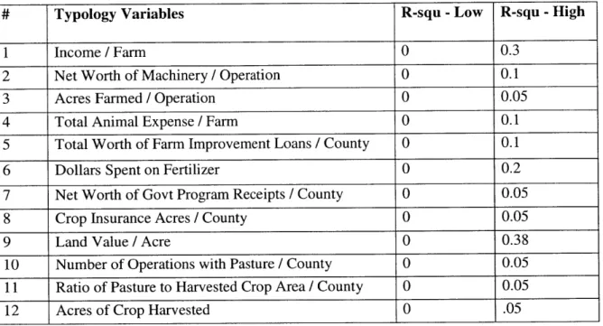
Initially to find basic relationships between yields, linear regression was done to relate county typology and management variables to yield. These results are summarized in tables 2 and 3. Table 2 shows the variables related and range for each, while table 3 shows which variables had the highest relation to a given crop.

Table 2 - List of regressed typology variables regressed against yield with range of R-square

# Typology Variables R-squ -Low R-squ - High

1 Income / Farm 0 0.3

2 Net Worth of Machinery / Operation 0 0.1

3 Acres Farmed / Operation 0 0.05

4 Total Animal Expense / Farm 0 0.1

5 Total Worth of Farm Improvement Loans / County 0 0.1

6 Dollars Spent on Fertilizer 0 0.2

7 Net Worth of Govt Program Receipts / County 0 0.05

8 Crop Insurance Acres / County 0 0.05

9 Land Value / Acre 0 0.38

10 Number of Operations with Pasture / County 0 0.05 11 Ratio of Pasture to Harvested Crop Area / County 0 0.05

12 Acres of Crop Harvested 0 .05

The results shown in table 2 suggest that the scatter in figures 1,2 and 3 is not strongly

management based. There was not one factor with a high rsquare value that was shown to have that effect for all crops. While it is important to note that certain rsquare values did show a link, those variables were also not necessarily describing a variable of interest (i.e. - a link between yield and income/farm was shown; yet profit is correlated with yield so this does not add to the discussion on its own). This indicates that there may be an effect but that it is likely crop specific and sporadic. Hence it appeared that management or typology was not a limiting factor in yield.

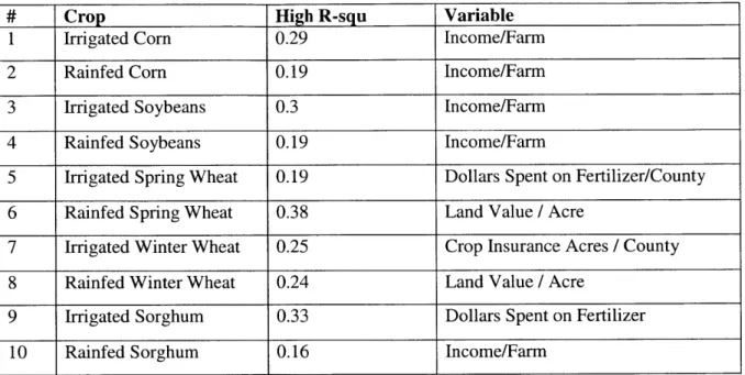
Table 3 - Crops and corresponding regression variables when regressed against the crop

that had the highest R-square value

# Crop High R-squ Variable

1 Irrigated Corn 0.29 Income/Farm

2 Rainfed Corn 0.19 Income/Farm

3 Irrigated Soybeans 0.3 Income/Farm

4 Rainfed Soybeans 0.19 Income/Farm

5 Irrigated Spring Wheat 0.19 Dollars Spent on Fertilizer/County

6 Rainfed Spring Wheat 0.38 Land Value / Acre

7 Irrigated Winter Wheat 0.25 Crop Insurance Acres / County 8 Rainfed Winter Wheat 0.24 Land Value / Acre

9 Irrigated Sorghum 0.33 Dollars Spent on Fertilizer

10 Rainfed Sorghum 0.16 Income/Farm

The results for environmental variables were such that nearly all the environmental variables had an rA2 that exceeded every typology and management variable. Given the scattered results and the links shown via environmental variables, it was decided that further analysis would consist only of environmental variables and analysis should be done over a smaller spatial area to attempt to isolate sources of variability.

The information in table 3 further supports the idea that effects of management are generally more context specific, and that links are not consistent across crop and variables.

Furthermore, it is possible that this may point to management factors in the US as being a moot point in the yield discussion. In the US there are over 2800 extension offices (spread across 3144 counties) that are partially tasked with informing farmers about best practices in raising crops and animals (National Pesticide Information Center, 2017). Therefore, there is a large network across which to promulgate information relating to best management practices. As noted by Anderson and Feder (2004), extension efforts can be key in initial dissemination of new information. Thus, it is arguable that given the large number of extension offices in the US and the modem access to information possessed by the typical citizen, that there is not substantial management gap between locations.

Also, given the non-limited access to fertilizers in the US, it is unlikely that farmers are hindered by lack of the fertilizer that they desire.

It is arguable that the lack of link with typology can be linked to management. For example, as noted by Cassman (1999), soil quality can be improved by management practices to obtain improved yields. Thus, if farmers are practicing up to date management then it would follow that differences in yield due to land value would be minimized.

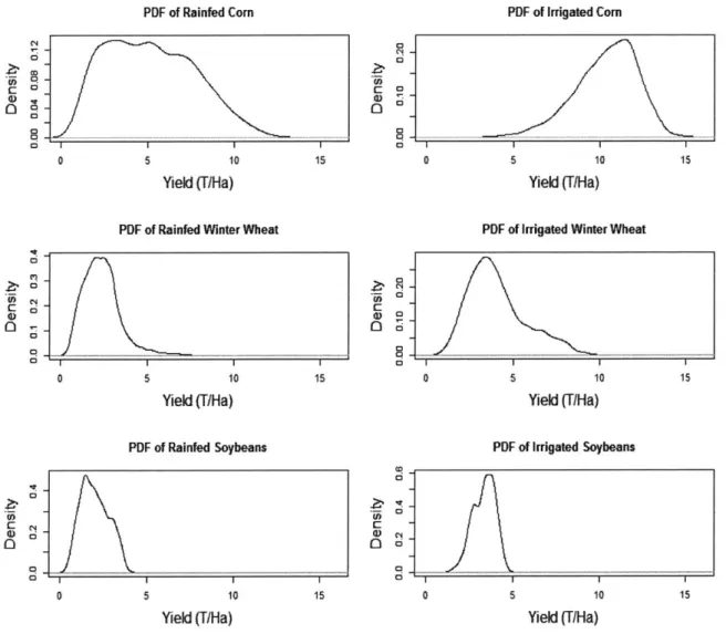
Also, to understand the distributions of the yields being studied, probability distributions (PDFs) were made. PDFs for three crops are shown in figure 4.

PDF of Rainfed Corn

II II

0 5 10 15 Yield (F/Ha)

PDF of Rainfed Winter Wheat

0 5 10 15 Yield (T/Ha) PDF of Rainfed Soybeans 5 10 Yield (T/Ha) 15 0 Z.i a) 0 0J ... 0 0 Ci 0 0 0 0 PDF of Irrigated Corn 0 5 10 15 Yield (T/Ha)

PDF of Irrigated Winter Wheat

0 5 10 15 Yield (T/Ha)

PDF of Irrigated Soybeans

0 5 10 15

Yield (T/Ha)

Figure 4 - Kernel Density Plots for 3 Major US Crops for 2000-2015

Nj 6-0 U) a) 0 a) 0 a) 0 ... J ... ...

.

.

...

Figure 4 consists of crop observations from the entire US where irrigated and rainfed yields are distinguished. Figure 4 summarizes the general trend for probability distribution of crops for all places observed. Irrigated yields had less spread than their rainfed counterparts with generally a higher mean. The results seemed to indicate a reduction in variability due to irrigation, but not as much as anticipated. Furthermore, the skew coupled with extended tails for both corn and wheat suggested that while these crops were on the average more consistent, they were subject to something that caused periodically large yield variation. If the earlier arguments for minimal effect from management and typology across areas were to hold true, then this would point to unique combinations of environmental variables that could not be damped out by access to moisture.

3.1.2 Yield and Environmental Variables

In the state of Nebraska, the variables of moisture and temperature were explored, and it was found that yield and physical attributes of the state follow the same general pattern. For example, as shown in figures 5-9 the structure average yield in Nebraska in corresponds generally with typical soil moisture and subsequently the soil type of the state, as well as with mean

temperature.

4.

Higher Capacity

Figure 5 - Relative Soil Water Holding Capacity for Nebraska Soils. (Wilhelmi and Wilhite, 2002) Areas with smallest capacities are primarily sandy soils.

Nebraska Growing Season Averages

Nebraska, 2000-2015

Mean, Daily, Air Temperature (Deg C)

16.330355 - 17.000000 17.000001 - 18.000000

18.000001 -19.000000 19.000001 -20.000000

20-000001 -21000000

Figure 6 -Average mean, daily air temperature for growing season in Nebraska from 2000-2015

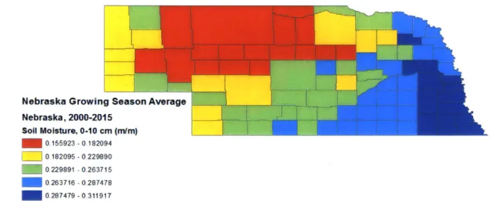
Nebraska Growing Season Average Nebraska, 2000-2015 Soil Moisture, 0-10 cm (mlm) 0.155923 -0.182094 0 182095 -0.229890 0.229891 -0.263715 0.263716 -0.287478 0-287479 -0-311917

Figure 7 - Average Soil Moisture distribution temperature for growing season in Nebraska from 2000-2015

Nebraksa Growing Season Averages Nebraska, 2000-2015

Rainfed Corn Yield (T/Ha)

-

[I]

E__I TJ

Figure 8 - Average Rainfed Corn Yield in Nebraska from 2000 - 2015

WI--Nebraska Growing Season Averages

Nebraska, 2000-2016 Irrigated Com Yield (lHa)

0.000000 - 1.500000 1-500001 -3000000 M 3000001 -4.500000 4 500001 -6.000000 6000001 -7 500000 7500001 -9.000000 9000001 -10-500000 10.500001 -12.000000 12-000001 - 13-500000

Figure 9 - Average Irrigated Corn Yield for Nebraska from 2000-2015

The maps shown in figure 5-9 indicate that there are patterns in yield that follow basic

environmental patterns. This is obvious for soil moisture wherein the drops in average soil moisture were accompanied nearly exactly for all counties by a drop in average yield. Also, the pattern between both irrigated and rainfed yields indicates that there is more than just soil

I-moisture affecting yields. Given the previous conclusion on the ability of farmers to amend the soils, that would seem to indicate that only then that available sunlight would be the primary help or hindrance when moisture is not limiting.

The basic relationships shown in the figures are reflected partially in the structure of the state. In figures 5-9, the right-hand portion, adjacent the border, is in the Missouri River valley. Hence it is in a relatively low portion of the state that has a large proportion of glacial influence

characterizing the soil.

Further to the left, in the portion of the state noted for having the lowest soil water holding capacity in figure 5 and a lower typical soil moisture shown in figure 7, the elevation begins to increase relative to the valley, and the soil becomes sandy. From right border to left border, there is a generally linear gradient from roughly 400 m to 1300 m above sea level. These both

contribute to a lower typical soil moisture, since not only does sand hold less water, but an increase in elevation generally means a decrease in annual precipitation, and a decrease in mean temperature which does hold true here.

Figures 5-9 indicate that there are patterns in yield that follow basic physical and environmental patterns, putting forth that at the very least there is a spatial organization of yield and

contributing variables. This is seen for soil moisture wherein the changes in average soil moisture are accompanied nearly exactly for all counties by a change in average yield. Yield patterns also, to a lesser extent, mimic temperature levels in both cases.

Furthermore, the uniform pattern between both irrigated and rainfed yields suggest that there is a pattern in yield that is not reflected by soil moisture. This would also suggest that the variability in both rainfed and irrigated crop yields is linked in some way.

This portion of the analysis indicated that there was potential for further understanding with regard to both soil moisture and temperature, which thus caused those two factors to be forwarded in to the LME analysis as the primary factors of interest.

3.1.3 Yield and Phenology

In considering corn, the phenology of the plant itself was found to be of importance. As shown in figure 10, the water use of corn peaks at the point when it starts it reproductive period and begins creating the grain that is harvested.