HAL Id: hal-01244264
https://hal.inria.fr/hal-01244264
Submitted on 15 Dec 2015HAL is a multi-disciplinary open access archive for the deposit and dissemination of sci-entific research documents, whether they are pub-lished or not. The documents may come from teaching and research institutions in France or abroad, or from public or private research centers.
L’archive ouverte pluridisciplinaire HAL, est destinée au dépôt et à la diffusion de documents scientifiques de niveau recherche, publiés ou non, émanant des établissements d’enseignement et de recherche français ou étrangers, des laboratoires publics ou privés.
Algorithmic differentiation applied to the optimal
calibration of a shallow water model
Félix Demangeon, Cédric Goeury, Fabrice Zaoui, Nicole Goutal, Valérie
Pascual, Laurent Hascoët
To cite this version:
Félix Demangeon, Cédric Goeury, Fabrice Zaoui, Nicole Goutal, Valérie Pascual, et al.. Algorithmic differentiation applied to the optimal calibration of a shallow water model. La Houille Blanche - Revue internationale de l’eau, EDP Sciences, 2015. �hal-01244264�
ALGORITHMIC DIFFERENTIATION APPLIED TO THE
1
OPTIMAL CALIBRATION OF A SHALLOW WATER MODEL
2 3 4
Félix DEMANGEON
(1), Cédric GOEURY
(2) 5Fabrice ZAOUI
(2), Nicole GOUTAL
(1) (2) 6Valérie PASCUAL
(3), Laurent HASCOËT
(3)7
(1)Laboratoire d’Hydraulique Saint-Venant (entité commune à EDF R&D, CEREMA et l’Ecole des Ponts), Chatou, France
8
(2)EDF R&D, Laboratoire National d’Hydraulique et Environnement (LNHE), Chatou, France - e-mail:
9
(3)
INRIA, (ECUADOR team), Sophia-Antipolis, France 10
Les informations de sensibilité fournies par les dérivées sont indispensables en science dans de nombreux
11
domaines. En analyse numérique, calculer très précisément la valeur des dérivées d’une fonction d’un
12
simulateur physique peut relever du défi. La méthode classique des Différences Finies (DF) est une solution
13
simple à mettre en œuvre pour estimer la valeur d’une dérivée. Cependant, elle reste très sensible
14
numériquement et coûteuse en temps de calcul. A contrario la méthode de la Différentiation Algorithmique
15
(DA) est une aide puissante pour le calcul des dérivées d’une fonction décrite au moyen d’un programme
16
informatique. Quelle que soit la complexité des algorithmes mis en œuvre dans l’expression d’une fonction, elle
17
calcule précisément sa dérivée en minimisant les efforts de développement.
18
Cet article montre l’apport de la DA en comparaison des DF sur le problème du calage d’un modèle hydraulique
19
à surface libre 1D de classe industrielle. Le calage du modèle est réalisé par un optimiseur mathématique
20
déterministe nécessitant le calcul précis de la sensibilité de la cote d’eau par rapport au frottement sur le fond
21
de la rivière. Deux cas tests réels de comparaison sont présentés. Ils permettent de valider la supériorité attendue
22
de la DA comme outil d’aide à l’obtention d’un calage optimal.
23
KEY WORDS: Modèle Hydraulique à surface libre, Calage, Différentiation Algorithmique
24
25
Algorithmic Differentiation for the optimal calibration of
26
a shallow water model
27
The information on sensitivity provided by derivatives is indispensable in many fields of science. In numerical
28
analysis, computing the accurate value of the derivatives of a function can be a challenge. The classical Finite
29
Differences (FD) method is a simple solution to implement when estimating the value of a derivative. However,
30
it remains highly sensitive numerically and costly in calculation time. Conversely, the Algorithmic
31
Differentiation Method (AD) is a powerful tool for calculating the derivatives of a function described by a
32
computer program. Whatever the complexity of the algorithms implemented in the expression of a function, AD
33
calculates its derivative accurately and reduces development efforts.
34
This article presents the contribution of AD in comparison to FD in the problem of calibrating an industrial
35
class 1D shallow water model. Model calibration is performed by a deterministic mathematical optimiser
36
requiring accurate calculation of the sensitivity of the water surface profile in relation to the friction on a river
37
bed. Two comparative real test cases are presented. They permit validating the better performance expected
38
from AD as a tool used to obtain optimal calibration.
39
KEY WORDS: Shallow Water Model, Calibration, Algorithmic Differentiation
40
I INTRODUCTION
41
Computing sensitivities of a numerical model is a key ingredient in Scientific Computing. The
42
derivatives that express these sensitivities must be computed with the best possible accuracy for applications
43
such as inverse problems, data assimilation, optimisation, or Uncertainty Quantification. When the model is
44
given as a computer program, several options exist to obtain its derivatives. Finite Differences (FD) is easily
45
implemented but returns approximate derivatives whose poor accuracy will degrade performance of the
46
complete application. A much better option is to create a new program that computes the exact, analytical
47
derivatives of the model. This new program can be written “by hand”, but this is a long and error-prone
process. Keeping the derivative model up to date with modifications of the original model is cumbersome.
49
Alternatively, Algorithmic Differentiation (AD) [Griewank and Walther, 2008] is a way to automate the
50
creation of the derivative program, thus providing accurate derivatives for a minimal development effort.
51
This article presents the application of the TAPENADE AD tool [Hascoët and Pascual, 2013] developed by
52
INRIA, on the 1D shallow water model MASCARET [Goutal et al., 2012]. It validates the use of the
53
differentiated code for an inverse problem of parameter estimation.
54
Regarding shallow water programs like MASCARET, the type of river bed is modelled by a friction
55
coefficient. This coefficient takes into account the friction of the fluid on the bottom as well as other
56
phenomena not modelled elsewhere such as turbulence and channel bends. This article presents the
57
application of AD to an inverse problem, namely the automatic calibration of the friction coefficient based
58
on a water surface profile measured during flooding at steady discharge. This permits testing both the AD
59
TAPENADE software with an industrial calculation code and improving the current method used to calibrate
60
the friction coefficient in MASCARET.
61
Initially, after having introduced the MASCARET 1D water flow calculation, the problem of calibrating
62
the friction coefficient is presented (cf. Section II). Section III focuses on the presentation of the optimisation
63
algorithm chosen to carry out this task. Then, Section IV describes the principle and use of AD. In Section V,
64
the results obtained from the different test cases are presented and discussed. Finally, the conclusions and
65
outlook are presented in Section VI.
66
II THE WATER MODELLING SYSTEM
67
The calculation code on which the works presented here is based is the MASCARET 1D free surface
68
modelling software. This software is part of the open-source hydro-computing system
TELEMAC-69
MASCARET (www.openmascaret.org). Applications of this system are many, from flood modelling and
70
flood plain modelling to the calculation of flood waves resulting from dam breaches, sediment transport and
71
water quality. It is composed of three main kernels: steady subcritical flow, unsteady subcritical flow and
72
unsteady super-critical flow. The steady subcritical flow kernel is the target of this study.
73
II.1 Saint-Venant 1D equations
74
As mentioned above, we focus only on 1D steady flows. The equations governing this type of flow are 1D
75
Barré St-Venant equations given by the following formulations [Chanson, 2004]:
76 a q = x Q (1) 77 a s f
+
S
)
+
q
gA(S
=
x
Z
gA
+
A
Q
x
2 (2) 78whereArepresents the wetted section (m2), Qthe flow rate (m3/s),
a
q
the inflow, Zthe free water surface79
(m), Sf the head losses resulting from the friction of the fluid on the walls,
S
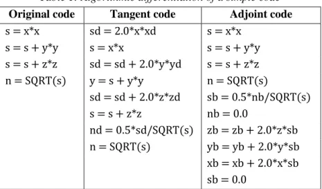
sthe singular head losses80
(narrowing, etc.).
81
Term
S
f of the momentum equation (2) is calculated using empirical friction laws such as that of Strickler82
(19th century) whose relation is given below:
83 3 / 4 2 2 2
R
A
K
Q
=
S
f (3) 84whereRdenotes the hydraulic radius (wetted surface divided by the wetted perimeter in m) andK, the
85
Strickler coefficient modelling the nature of the channel bed (m1/3
/
s).86
In the MASCARET hydraulic calculation, the river bed is divided into two zones, the main channel and the
87
flood plain. The main channel is the main flow zone. The flood plain is the secondary zone: this zone
88
participates in the flood flow, though it has a specific friction coefficient due to the different natures of the
89
soils. This coefficient is defined by the cross-section and by the bed, and is constant per friction zone, whose
90
sizes and numbers are determined by the study data. The friction coefficient takes into account the friction of
91
the walls on the fluid and the dissipation phenomena not modelled elsewhere (turbulence, etc.). Thus it
92
cannot be determined directly by the study data and must be adjusted using the water surface profiles
measured for a given flow rate. Done manually, this model calibration step is time consuming, but it is
94
indispensable to ensure the quality of the study. That is why an automatic calibration method using measured
95
elevation data has already been integrated in MASCARET.
96
This automatic calibration method is based on a first order unconstrained optimisation method known as
97
“gradient descent optimisation”, with a gradient approximated by finite difference. The disadvantages of this
98
approach are:
99
The velocity of convergence to the minimum sought can prove slow.
100
In certain cases, its accuracy can be poor.
101
The values of the friction coefficients obtained can exceed the values prescribed.
102
Therefore the objective of this work is to propose a more efficient automatic calibration algorithm
103
capable of eliminating the limitations mentioned, using Algorithmic Differentiation methods.
104
II.2 Automatic calibration
105
Automatic calibration is an inverse method used to find an “admissible” constant friction coefficient K
106
per zone, resulting in the calculation of a water surface profile close to the water surface profile measured for
107
a steady flow. The optimal search for this coefficient is done by minimising a cost function calculating the
108
difference between the level computed by the numerical model and the measured level:
109
flood N = c c meas N = j calc j meas j c j Z Z K = K J 1 1 2 ) ( ) (
(4) 110whereNfloodrepresents the number of floods, Nmeasc the number of measures linked to these floods,
α
cj a111
weighting coefficient that can be set to less than 1 when a measure is deemed uncertain,
Z
measj the water112
level measured at point j and Zcalcj the height calculated by the model.
113
Generally, optimisation methods are used to solve minimisation problems. The former can be very
114
different according to the form of the function to be minimised (convex, quadratic, nonlinear, etc.), its
115
regularity and the dimension of the space studied [Nocedal and Wright, 2006]. Many deterministic
116
optimisation methods are known as gradient descent methods, among which the best known is the Newton
117
method, which is the approach used in this work [Gilbert and Lemaréchal, 1989]. This minimisation process
118
will quickly find, when successful, a better solution in comparison with the value of the initial guess.
119
III THE BFGS QUASI-NEWTON METHOD
120
As mentioned above, the optimisation method chosen to minimise the cost function (4) is based on the
121
application of the Newton method to the gradient of the functional
J
, to find the zeros and then the extremes,122
thus the minimum. This method involves the calculation of the first and second derivatives of the cost
123
function. The main disadvantage of this type of approach is the use of the second derivative (Hessian) of the
124
cost function
2J
(
K
)
. Indeed, at each iteration of the Newton algorithm, it is necessary to calculate the125
Hessian and solve a linear system of the matrix
2J
(
K
)
. For large problems, the resolution of the linear126
system is out of reach. An alternative is to use algorithms such as the Quasi-Newton algorithm which
127
provides Hessian approximations that improve as the iterations progress, for a reasonable cost. Therefore the
128
method chosen to perform this work is the constrained Broyden Fletcher Goldfarb Shanno Quasi-Newton
129
Method (BFGS).
130
Using a constrained optimisation method makes it possible to impose boundaries when seeking the
131
parameter to be calibrated. Although the friction coefficient takes into account dissipation phenomena that
132
cannot be represented in the numerical model, it is directly dependent on the type of surface composing the
133
river bed. Thus an interval of acceptable “physical” values exists for searching the friction coefficient as a
134
function of the type of soil.
135
The optimisation method used involves calculating the gradient of the cost function. One could compute an
136
accurate gradient by manually differentiating the calculation code. However this would be time-consuming
137
and error-prone, as this implies writing a code of a size similar to the original code (more than 10,000 lines
of FORTRAN for MASCARET steady flow kernel). Nonetheless, AD software tools can alleviate this cost
139
[Griewank and Walther, 2008].
140
IV ALGORITHMIC DIFFERENTIATION
141
Algorithmic Differentiation of programs is a powerful technique for evaluating the derivatives of functions
142
described by computer programs. Contrary to traditional approaches, such as derivation by finite differences,
143
AD provides accurate derivatives at a relatively cheap cost, for a simple mathematical formula as well as for
144
a program with more than 100000 lines of code. By calculating an exact derivative, AD thus plays a key role
145
in developing a new optimisation method for the automatic calibration of the friction coefficient. This
146
section describes the principle of AD. Then, after having presented the TAPENADE software [Hascoët and
147
Pascual, 2013], used to differentiate the kernel of the steady calculation of MASCARET, its application is
148
described in the framework of implementing the optimal calibration of a shallow water model [Cunge et al.,
149
1980; Fread and Smith, 1978].
150
IV.1 Principle of Algorithmic Differentiation
151
Every calculation program, or at least its run-time trace, can be seen as a sequence of assignments
152
involving only unary (trigonometric function, square root, etc.) and binary (additions, multiplications, etc.)
153
operations. Therefore, the program can be seen as a composition of elementary functions, to which one can
154
apply the chain rule of calculus to obtain its derivative with analytic accuracy.
155
Consider a mathematical function F:
156 Y X F n m : (5) 157
Assume F is implemented as a sequence of rcomputer program instructions, each of them implementing
158
an elementary function. Call
f
l the elementary function corresponding to instructionl
:159
(X)
f
f
f
=
F(X)
=
Y
r r 1 1...
(6) 160By applying the chain rule of calculus to equation (6), the Jacobian matrix A of F, which is a
m
n
161matrix, writes as the product of the derivatives of the
f
l.162
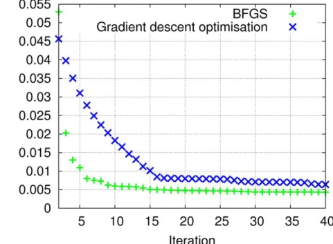
(X)
X
f
)
(x
x
f
)
(x
x
f
)
(x
x
f
=
(X)
X
F
=
A(X)
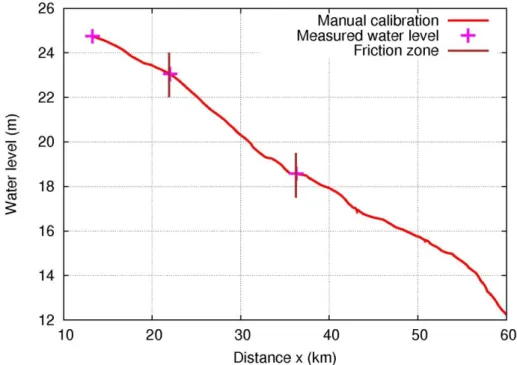
r r r r r r
1 1 1 2 2 2 1 1 1.
.
(7) 163Explicit evaluation of equation (7) can be extremely costly, as each derivative involved is a matrix roughly
164
of sizeqq, where q is the number of elementary variables active at the time of the instruction, i.e. of the
165
order or larger than m and n. Therefore, AD rather focuses on computing two useful projections ofA, from
166
which it may even be easier to retrieve the full A if necessary. This results in the two so-called “modes” of
167
AD:
168
The tangent mode computes δY=A.δX for any arbitrary vector δXn . In other words, it
169
computes a directional derivative which is the first-order variation of the output for a small
170
variation of the input in direction
δX
. From equation (7), it is clear that δY=A.δX is most171
efficiently computed from right to left, leading to only matrix-vector products. The total cost of
172
evaluating
δY
is only a small multiple of evaluating F. IfδX
is taken as an element of the173
Cartesian basis,
δY
is a column of the Jacobian A. The full A can be obtained by repeated calls174
to the tangent code on the input space's Cartesian basis. Notice that tangent mode implies the same
175
computation order as the original program, and therefore derivative computations can be
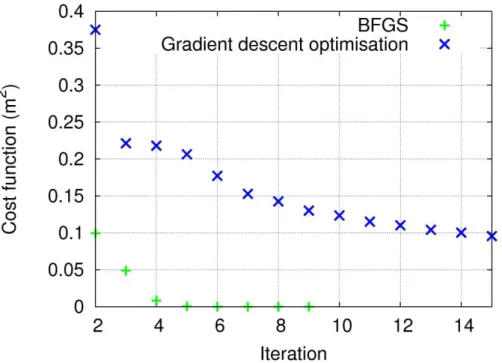
176
introduced into the original code by inserting a derivative instruction before each original
177
instruction. Implementation of the tangent mode is therefore straightforward. Table 1 (middle)
178
shows the tangent differentiated code of a simple code shown on the left, which computes the
179
norm of a 3D vector. Derivative variable names are built with an appended “d”. One can see the
180
straightforward structure of the tangent code. This tangent code must be run three times to obtain
181
the three components of the gradient.
The adjoint mode computes δ*X=δ*Y.A for any arbitrary (transposed) vector δ*Ym. In other
183
words it computes the gradient with respect to X of a scalar function, which is the weighted sum
184
of all elements of Y with weightings δ*Y . From equation (7), it is clear that δ*X is most
185
efficiently computed from left to right, since this leads only to vector-matrix products. Just like for
186
the tangent mode, the total cost of evaluating δ*X
is only a small multiple of evaluating F. If
187
Y δ*
is taken as an element of the Cartesian basis, δ*X is a row of the Jacobian A. The full A
188
can be obtained by repeated calls to the adjoint code on the output space's Cartesian basis.
189
Therefore, the adjoint mode tremendously outperforms the tangent mode when m=1, which is
190
the case in most optimization or inverse problems applications. The computation order for the
191
derivatives is reversed from the original program's order, which makes implementation of the
192
adjoint mode a technical challenge (see [Hascoët and Pascual, 2013]). In particular, intermediate
193
values from the original computation must be made available to the derivative computation in
194
reversed order, leading to difficult memory problems and trade-offs [Naumann, 2012]. Table 1
195
(right) shows the adjoint differentiated code of the same simple code. Derivative variable names
196
are built with an appended “b”. One can see the reversed structure of the adjoint code, and the
197
somewhat counter-intuitive shape of the derivative instructions. However, this adjoint code returns
198
the three components of the gradient in only one run.
199 200
Table 1: Algorithmic differentiation of a simple code 201
Original code Tangent code Adjoint code
s = x*x sd = 2.0*x*xd s = x*x s = s + y*y s = x*x s = s + y*y s = s + z*z sd = sd + 2.0*y*yd s = s + z*z n = SQRT(s) y = s + y*y n = SQRT(s) sd = sd + 2.0*z*zd sb = 0.5*nb/SQRT(s) s = s + z*z nb = 0.0 nd = 0.5*sd/SQRT(s) zb = zb + 2.0*z*sb n = SQRT(s) yb = yb + 2.0*y*sb xb = xb + 2.0*x*sb sb = 0.0 202
For further details on AD and the associated research, the reader can refer to [Griewank and Walther,
203
2008], [Naumann, 2012], to the proceedings of the AD conferences, and to the AD community website
204
www.autodiff.org.
205
IV.2 Algorithmic Differentiation implementation approaches
206
AD tools rely mostly on two different approaches, Operator Overloading and Source Transformation:
207
The Operator Overloading approach is possible only on languages that support overloading, such as
208
C++, ADA and FORTRAN 90. Examples of AD tools of this kind are ADOL-C [Walther and
209
Griewank, 2012], and dco [Lotz et al., 2011]. This AD method is the simplest to implement, since
210
it requires only the definition of a new data-type, and of the overloaded arithmetic operations on
211
this data type. Changes to the original code are minimal. However, efficiency is limited by the
run-212
time overhead of the overloading mechanism, and the reversed nature of the adjoint mode
213
contradicts the natural order of overloading, causing extra run-time and memory overhead;
214
The Source Transformation approach is used for instance in the tools TAF [Giering et al., 2005],
215
ADIC [Bischof et al., 1997], ADIFOR [Bischof et al., 1991], OpenAD [Utke et al., 2008], and
216
TAPENADE [Hascoët and Pascual, 2013]. These tools target mainly C and Fortran 90 programs.
217
Source transformation uses concepts from compilation, for example the generation and
218
transformation of abstract syntax trees. Like in a compiler, the source program is parsed, analysed,
and then transformed into a new differentiated source program. Sophisticated compilation
220
techniques allow for optimisations that improve performance of the differentiated code.
221
IV.3 The TAPENADE AD tool
222
The AD tool chosen for this work is TAPENADE, developed by the ECUADOR team of INRIA [Hascoët
223
and Pascual, 2013]. Tapenade is based on the source transformation approach. It globally analyses the code
224
to which it is applied and fully rebuilds a differentiated program, adding instructions into the original
225
program. It applies to both FORTRAN 90 and C. TAPENADE provides both tangent- and adjoint-mode AD.
226
One reason for our choice is the direct access to the differentiated source, providing much flexibility and the
227
opportunity to optimise the execution time of the adjoint by adjusting the differentiated program.
228
Collaboration between EDF and INRIA helped in applying TAPENADE to MASCARET and provided
229
feedback and experience on the problems encountered, thus bringing improvements to both tools.
230
IV.4 Application of TAPENADE to MASCARET
231
IV.4.1 Context
232
As mentioned in section II.2, the search for an optimal friction coefficient during automatic calibration
233
must be done by minimising the cost function (4). In our calibration experiments, we calibrate K defined as
234 i
K
for each friction zone i, whereas what the simulation uses is an expanded expK defined at each node235
p. By definition, for all node p belonging to friction zone i:
236
i p K
expK (8)
237
The cost function (4) becomes:
238
flood N = c c meas N = j calc j meas j c jZ
Z
expK
K
α
=
(K)
J
1 1 2))
(
(
ˆ
(9) 239The gradient of Jˆ with respect to K is:
240
flood N = c c meas N = j calc j calc j meas j c jdK
dexpK
dexpK
dZ
K
expK
Z
Z
α
=
dK
J
d
1 1))
(
(
2
ˆ
(10) 241where
Z
calcj is the water surface profile calculated from expK by the model. The matrixdK dexpK
has a
242
very simple structure, with one row per node and one column per friction zone. For each friction zone i, this
243
column elements are 1 for nodes
p
belonging to i and 0 otherwise.244
IV.4.2 Choice of the AD mode 245
The largest and most computationally-intensive part of equation (10) is the derivative of the water surface
246
calculated at each point
j
of the grid as a function of the friction coefficients at each node:247
dexpK dZcalcj
(11)
248
As is usually the case, it is fortunately not needed to compute this large matrix explicitly. Equation (10)
249
actually amounts to multiplying this matrix on the left and on the right as follows:
250
on the left, it is multiplied with a single-row matrix, i.e. a transposed vector, whose element of rank
251
j
is: 252
flood N c calc j meas j c j Z Z expK K 1 ))) ( ( ( 2
(12) 253assuming there is a measurement available at each point. If not, set
cj to 0. on the right, it is multiplied with
dK
dexpK
which has one column per friction zone. Our first
255
applications have only a few friction zones.
256
As the left multiplier is a single-row matrix, we are aware that adjoint differentiation can compute the
257
complete dK
J d ˆ
in a single run of the adjoint code. On the other hand, since the right multiplier has one
258
column per friction zone, the code produced by tangent differentiation must run once per friction zone to
259
compute the full dK
J d ˆ
.
260
However, our first applications have less than 10 friction zones and experience shows that adjoint codes
261
are almost always 2 to 5 times slower than tangent codes, due to their sophisticated architecture. Moreover,
262
the present architecture of MASCARET doesn’t lend itself easily to isolating the computation of the left
263
row-vector multiplier. For these reasons, we feel it is wise to use the tangent mode of AD for our first
264
calibration experiments, and in the future slightly refactor MASCARET and switch to the adjoint mode when
265
it comes to larger cases.
266
IV.4.3 Actual differentiation and derivatives validation 267
Actual differentiation by TAPENADE of the steady subcritical kernel of MASCARET requires some
268
technical adaptions, as is often the case for codes of this size (
140000
lines of code). Differentiation itself269
produces a long message log, most of which can be discarded after a first careful look. The remaining
270
messages are about limitations of the AD tool that must be worked around by modifying the source (e.g.
271
array initializations), or limitations of AD that require post-processing of the differentiated code. In the latter
272
category, differentiation of MASCARET introduces temporary arrays for intermediate variables and boolean
273
masks, whose size could not be determined at differentiation time. The end-user is requested to provide these
274
sizes in a special-purpose separate module.
275
As a research tool, TAPENADE also contains a number of errors. Collaboration between the AD tool
276
developers and MASCARET developers is essential, resulting often in improvements to the AD tool and
277
sometimes in clarifications to the MASCARET source.
278
When it finally compiles, the differentiated code must be incorporated in a calling context which is similar
279
to that of the original code, except for additional variables that hold the input and output derivatives. This
280
can be seen as the task of the final user but on this occasion we could test an experimental feature of the AD
281
tool which generates a new calling context from the existing one by declaring, allocating, initializing and
282
freeing the differentiated variables. This is an ongoing development, as adjoint differentiation of dynamic
283
memory management is still an active research subject.
284
Once the differentiated code actually produces derivatives, it is necessary to check their correctness.
285
Validation of the derivatives is usually performed in two steps:
286
Validation of the tangent derivatives produced by AD, against derivatives approximated by Finite
287
Differences.
288
Validation of the adjoint derivatives against the (validated) tangent derivatives. Reusing the notation
289
of section IV.1, given any two vectors
δX
and δ*Y, the scalarδ .A.
*Y
δX
can be computed in290
two ways, either through tangent mode or through adjoint mode. The result must be the same up to
291
machine precision.
292
We performed these two tests on MASCARET for the steady river test cases, with satisfying results. Even
293
if for this work, we decided not to use the adjoint for the final calibration experiments, we did validate both
294
tangent and adjoint codes:
295
The maximum difference between the gradient calculated by FD and that obtained by AD is of the
296
order of 104 .
297
The maximum difference observed between the gradient calculated by the tangent and adjoint modes
298
is of the order of machine precision (1014).
299
Finally, the runtime of the tangent code is roughly twice the run time or the original code, whereas the
300
adjoint code is roughly seven times slower than the original code. This varies with the test case but conforms
301
to what is commonly expected. This validates a posteriori our choice of using the tangent mode for the
following calibrations, and indicates to switch to the adjoint mode when calibrating a larger number of
303
parameters.
304
V VALIDATION OF THE AUTOMATIC CALIBRATION METHOD
305
In order to validate the automatic calibration method developed during this work, two cases of real
306
application were studied. Since the new algorithm allows bounding the search for optimal friction
307
coefficients, in order to avoid all outliers and non-physical values, it is performed in
25
to45
m1/3/
s for the308
main channel and in
5
to20
m1/3/
sfor the flood plain.309
The results obtained with the method developed here were compared with those obtained using the old first
310
order calibration method with a gradient calculated by FD. The comparison between the two approaches is
311
performed by focusing on the speed of convergence of the different methods used, the final value of their
312
cost function and, of course, the values of the friction coefficients obtained.
313
V.1 Calibration of the reach of the Rhone close to the Bugey nuclear power plant
314
V.1.1 Context and available data
315
This first case study corresponds to a 5 km section of the Rhone River located near the Bugey nuclear
316
power plant. Upstream and downstream of the model, the boundary conditions used are the imposed flow
317
rate and water level, respectively. In addition, for this case, 30 inflows distributed along the river were taken
318
into account. The geometry of this calculation case is not described as it not the purpose of the present study.
319
Regarding the calibration, 8 friction zones of variable size were considered and 28 water level measures
320
were available (cf. figure 1) for an upstream flow rate of 446 m3/s and a downstream water level of 188.10
321
m. Since the upstream flow rate for which observations were available was relatively low, the flow regime
322
studied was non-overtopping. Therefore, only the friction coefficients of the main channel could be
323
calibrated.
324
Furthermore, since this case had already been the subject of a study, calibration data obtained manually
325
were also available. The Strickler coefficient values per friction zone calibrated manually were (43 / 28.5 /
326
39 / 34 / 45 / 27 / 35 / 35) m1/3
/
s.327
V.1.2 Comparison of results obtained during automatic calibration
328
The purpose of this paragraph is to compare the results obtained with:
329
The automatic calibration method using the BFGS optimisation method.
330
The former calibration method using the gradient descent optimisation method.
331
A reference manual calibration.
332
Figure 1 presents the water surface profiles obtained for these three different calibration methods. For the
333
two automatic calibration methods, the Strickler coefficient was initialised at a value of 30 m1/3
/
s in each334
zone.
335 336
337
Figure 1: Water height calculated using the friction coefficients of the main channel calibrated manually
338
and automatically (BFGS, gradient descent optimisation). 339
As shown in the figure above, the results obtained from the three calibration methods are very similar for
340
the water surface profile calculated. This confirms the methodological choices that we present in this
341
document.
342
Figure 2 shows the friction coefficient values obtained with the three methods.
343
344
Figure 2: Friction coefficient values by zone obtained with the three different calibration methods.
345
From Figure 2, we draw the following observations:
346
The values resulting from the manual and automatic calibrations making use of the BFGS
347
optimisation method are, generally speaking, quite close (about 10% in terms of relative error).
348
The magnitude of variability of the Strickler coefficients between two consecutive friction zones is
349
greater for the two previous methods than for automatic calibration method using the gradient
350
descent optimisation method.
The three calibration methods present an almost identical Strickler coefficient for the last friction
352
zone.
353
The last comment permits understanding why, despite the different sets of friction coefficients, the water
354
surface profiles calculated are quite close for the three calibration methods. It is very clear in the light of
355
these results that the downstream friction zone is that which has the greatest impact on the calibration of this
356
case study. This can be explained, on the one hand, by the size of this friction zone, which comprises about 3
357
km of the 5 km of the section studied; and on the other hand, by the resolution method used in the steady
358
subcritical flow kernel of MASCARET which is performed from downstream to upstream for the calculation
359
of the water surface profile along the length of the section studied. Furthermore, the results shown in Figure
360
2 emphasise the complexity of determining a set of optimal friction coefficients. Indeed, the uniqueness of a
361
solution of this type of problem is not mathematically proven and different sets of parameters can give
362
analogous results. Thus it is important to set bounds on the search for optimal friction coefficients to avoid
363
all the outliers and non-physical values. This is why the automatic calibration method developed here uses a
364
constrained optimisation approach.
365
Regarding the speed of convergence of the two automatic calibration methods (BFGS and gradient descent
366
optimisation), Figure 3 highlights a faster convergence and accuracy for the automatic calibration method
367
developed in this work in comparison to the old method. The BFGS method based on AD finds an optimal
368
solution in less than 10 iterations whereas the old method reaches an equivalent result in 40 iterations. The
369
manual calibration requires approximately 20 simulation runs to find a cost function between 10-1 and 10-2.
370
For the total computation time, there is no noticeable difference to reach the same accuracy on the cost
371
function for both methods.
372
373
Figure 3: Value of the cost function according to number of iterations for the Quasi-Newton BFGS method
374
and the gradient descent optimisation method. 375
To conclude this first case of implementation, the automatic calibration method based on the constrained
376
optimisation approach of the Quasi-Newton method BFGS presented better accuracy (after 40 iterations, the
377
cost functions are constant with a value 4.3103 m2 for the BFGS approach versus 6.4103m2 for the
378
gradient descent optimisation method) with faster convergence in comparison to the old method used.
379
To compare these initial findings, a second application case study was tested. It takes a 50 km section of
380
the Garonne River and includes both the main channel and the flood plain.
V.2 Calibration of a reach of the Garonne
382
V.2.1 Context and available data
383
The zone selected to perform this study was a section of the Garonne River between Tonneins, downstream
384
of the confluence with the Lot River, and La Réole (limit of the hydrodynamic influence of the tide), i.e.
385
about 50 km of river [Besnard and Goutal, 2011].
386
Upstream and downstream of the model, the boundary conditions used were imposed flow rate and water
387
surface profile, respectively. The section studied was divided into 3 friction zones of variable size (cf. Figure
388
4).
389
To calibrate this case, two sets of flood data each composed of 3 measures were available. The first set of
390
data concerned a non-overtopping flood with a flow rate of 255 m3/s and a downstream height of 4 m
391
whereas the second set resulted from an overtopping flood with a flow rate of 2550 m3/sand a downstream
392
height of 11.73 m. The geometry of the model is not described in this paper.
393
Furthermore, since this case had already been the subject of a study, the calibration data obtained manually
394
were also available. The Strickler coefficient values per friction zone calibrated manually were, for main
395
channel and the flood plain, (40/32/33) m1/3/s and (10/12/12) m1/3/s, respectively. The water surface profile
396
linked to these friction coefficient values is shown in the figure below:
397
398
Figure 4: Water surface profile calculated with friction coefficients calibrated manually.
399
V.2.2 Comparison of results obtained during automatic calibration
400
For the two automatic calibration methods, the Strickler coefficients of the main channel and flood plain
401
were initialised at the values of 30 m1/3/s and 15 m1/3/s respectively, in each zone. In this case, the automatic
402
calibration determined the friction coefficients of the main channel and flood plain simultaneously with the
403
two floods available.
404
The results obtained with the two automatic calibration methods are presented in the following figure:
405 406 407
408
Figure 5: Friction coefficient values of the main channel and flood plain obtained with different automatic
409
calibration approaches. 410
The first two observations mentioned in the presentation of the results of the previous test case remain
411
valid for this new application.
412
However, in comparison to the previous case, the results shown in Figure 5 highlight the need to set
413
bounds when searching for the friction coefficient. Indeed, the friction coefficient value for a natural flood
414
plain must be between 5 and 20 m1/3/s. In this case of application, contrary to the automatic calibration
415
method based on the constrained BFGS Quasi-Newton method, this criterion is not complied with in the
416
calibration based on the gradient descent optimisation method, for which the friction coefficient of the flood
417
plain which extends from 13150 m to 21925 m was found equal to 31 m1/3/s.
418
Regarding the speed of convergence of the two automatic calibration methods (BFGS and gradient descent
419
optimisation), Figure 6 also highlights higher accuracy and speed of convergence for the number of
420
iterations, for the automatic calibration based on the Quasi-Newton BFGS optimisation method than for the
421
old method. After only 9 iterations, the cost function was 7106m2 for the BFGS method versus 0.14 m2
422
for the gradient descent optimisation method. This last value is too high to consider the found Strickler
423
coefficients as acceptable.
425
Figure 6: Cost function values according to the number of iterations obtained with the different automatic
426
calibration approaches. 427
The case of the Garonne emphasised the efficiency of the constrained BFGS Quasi-Newton method when
428
calibrating friction coefficients in the framework of a river, on the one hand by bounding the minimisation
429
and on the other hand providing better accuracy and convergence speed.
430
V.3 Synthesis: contribution of AD to the automatic calibration
431
The real test cases of Bugey and Garonne show the superiority of the second order BFGS method over the
432
first order gradient method as expected. Even if the cost function of the BFGS method is always smaller than
433
for the gradient method, it is not easy to set a value of convergence criteria for the cost function from a
434
practical point of view. This mainly depends on the number of floods/measurements and on the required
435
accuracy for the computed water levels. Consequently, practical applications can have a wide range of values
436
for the convergence criteria.
437
Finally, in order to see more clearly the gain of using AD, the BFGS method is tested on a new set of data
438
with FD. The following table compares the cost function values for 15 iterations of the BFGS algorithm.
439 440
Table 2: Influence of the derivative method on the BFGS algorithm 441
BUGEY GARONNE
FD AD FD AD
6.0910-3 4.2110-4 6.3910-1 3.9810-10 VI CONCLUSIONS AND OUTLOOK
442
Evaluating derivatives for a given function (mathematical function and calculation code) can be a
443
challenge. Algorithmic Differentiation proves a powerful technique for evaluating the derivatives of
444
functions described by computer programs [Griewank and Walther, 2008].
445
This article presented the application of the AD tool TAPENADE [Hascoët and Pascual, 2013] to one of
446
the hydraulic codes of MASCARET [Goutal et al., 2012], and validated its use for an inverse parametric
447
optimisation problem. For 1D hydraulic programs like MASCARET, the nature of a river bed is modelled by
448
a friction coefficient. This coefficient accounts for the friction of walls on fluid as well as other phenomena
449
not modelled elsewhere such as turbulence and channel bends. The objective of this work was to apply AD
450
to the inverse problem of optimal friction coefficient calibration.
451
Automatic calibration is an inverse method used to obtain a constant “admissible” friction coefficient per
452
zone, resulting in the calculation of a water surface profile close to that measured for a steady flow. The
optimal search for this coefficient takes the form of minimising a cost function calculating the difference
454
between the height calculated by the numerical model and the measured height. This led to choosing the
455
constrained BFGS Quasi-Newton method to minimise the cost function. Using a constrained optimisation
456
method allowed setting bounds when searching the parameter to be calibrated. The optimisation method
457
employed involved calculating the gradient of the cost function, which was obtained through AD of the
458
calculation code.
459
The results obtained with the method developed were compared with those obtained with an old calibration
460
method based on the gradient descent optimisation method with a gradient approximated by FD. The
461
comparison was performed on two real case studies.
462
These two cases of application highlighted the efficiency of the constrained BFGS Quasi-Newton method
463
during the calibration of friction coefficients in comparison to gradient descent optimisation due to the
464
setting of bounds for minimisation. Indeed, searching an optimal friction coefficient calibration is a complex,
465
sometimes ill-posed problem for which different sets of parameters can provide analogous results. This
466
question has not been investigated here, but to avoid any outliers or nonphysical values, it is important to set
467
bounds on the search for optimal friction coefficients. Furthermore, in the light of the different results
468
presented, the speed of convergence of the new calibration method is faster in terms of iterations and better
469
accuracy is obtained. The automatic calibration method developed during this work will therefore be
470
deployed in the upcoming version of the MASCARET software (version 8.1).
471
For several decades, EDF R&D has developed numerical codes to respond to the problems encountered by
472
the company. Innovative techniques such as AD may fit into the constant improvement of these tools.
473
AD covers a wide array of applications. This work was conducted in the framework of inverse problems.
474
However, other applications will also be explored:
475
Quantification of uncertainty. Certain methods allow exploring the range of variation of calculation
476
code inputs using partial derivatives to deduce global sensitivity indices.
477
Variational data assimilation methods (“4DVAR” algorithm). As with automatic calibration, this
478
type of algorithm requires the use of an optimisation method which in turn requires calculating the
479
gradient of a cost function.
480 481
VII REFERENCES
482
Besnard A., Goutal N. (2011) – Comparison between 1D and 2D models for hydraulic modeling of a
483
floodplain: case of Garonne river. La Houille Blanche, 3: 42-47
484
Bischof C. H., Roh L., Mauer-Oats A. J. (1997) – ADIC: an extensible automatic differentiation tool for
485
ANSI-C. Software: Practice and Experience, 27(12): 1427-1456.
486
Bischof C. H., Carle A., Corliss G. F., Griewank A., Hovland P. D. (1991) – ADIFOR – Generating
487
Derivative Codes from Fortran Programs. Scientific Programming, 1: 11-29.
488
Chanson H. (2004) – Environmental hydraulics of open channel flows. Elsevier Butterworth-Heinemann.
489
Cunge J. A., Holly F. M., Verwey A. (1980) – Practical aspects of computational river hydraulics. Pitman
490
Advanced Publishing Program.
491
Fread D. L., Smith G. F. (1978) – Calibration technique for 1-D unsteady flow models. Journal of Hydraulics
492
Division. Proceedings of the ASCE, 104(HY7): 1027-1044
493
Giering R., Kaminski T., Slawig T. (2005) – Generating efficient derivative code with TAF: Adjoint and
494
Tangent linear Euler flow around an airfoil. Future Generation Computer Systems 21(8): 1345-1355
495
Gilbert J.-C., Lemaréchal C. (1989) – Some numerical experiments with variable-storage quasi-Newton
496
algorithms. Mathematical Programming, 45(1-3): 407-435
Goutal N., Lacombe J.-M., Zaoui F., El Kadi Abderrezzak K. (2012) – MASCARET : a 1-D open-source
498
software for flow hydrodynamic and water quality in open channel networks. River Flow, Murillo (Ed.),
499
Taylor & Francis Group, London, 1169-1174. 500
Griewank A., Walther A. (2008) – Evaluating derivatives: Principles and Techniques of Algorithmic
501
Differentiation. Society for Industrial and Applied Mathematics. 502
Hascoët L., Pascual V. (2013) – The Tapenade Automatic Differentiation tool: Principles, Model and
503
Specification. ACM Transactions on Mathematical Software, 39(3): 20:1-20:43.
504
Lotz J., Leppkes K., Naumann U. (2011) – dco/c++ - Derivative Code by Overloading in C++. Aachener
505
Informatik-Berichte (AIB)
506
Naumann U. (2012) – The Art of differentiating Computer Programs. An Introduction to Algorithmic
507
Differentiation. SIAM-Society for Industrial and Applied Mathematics. 508
Nocedal J., Wright S. J. (2006) – Numerical Optimization. Springer Series in Operations Research and
509
Financial Engineering. Springer.
510
Utke J., Naumann U., Fagan M., Tallent N., Strout M., Heimbach P., Hill C., Wunsch C. (2008) –
511
OpenAD/F: A modular, open-source tool for Automatic Differentiation of Fortran codes. ACM
512
Transactions on Mathematical Software, 34(4): 18:1-18:36. 513
Walther A., Griewank A. (2012) – Getting started with ADOL-C. Combinatorial Scientific Computing. U.
514
Naumann and O. Schenk (Ed.), 181-202 515