HAL Id: insu-01175722
https://hal-insu.archives-ouvertes.fr/insu-01175722
Submitted on 7 Apr 2016
HAL is a multi-disciplinary open access
archive for the deposit and dissemination of
sci-entific research documents, whether they are
pub-lished or not. The documents may come from
teaching and research institutions in France or
abroad, or from public or private research centers.
L’archive ouverte pluridisciplinaire HAL, est
destinée au dépôt et à la diffusion de documents
scientifiques de niveau recherche, publiés ou non,
émanant des établissements d’enseignement et de
recherche français ou étrangers, des laboratoires
publics ou privés.
Estimate of the erosion rate from H2O mass-loss
measurements from SWAN/SOHO in previous
perihelions of comet 67P/Churyumov-Gerasimenko and
connection with observed rotation rate variations
Jean-Loup Bertaux
To cite this version:
Jean-Loup Bertaux.
Estimate of the erosion rate from H2O mass-loss measurements from
SWAN/SOHO in previous perihelions of comet 67P/Churyumov-Gerasimenko and connection with
observed rotation rate variations. Astronomy and Astrophysics - A&A, EDP Sciences, 2015, 583, A38
(10 p.). �10.1051/0004-6361/201525992�. �insu-01175722�
A&A 583, A38 (2015) DOI:10.1051/0004-6361/201525992 c ESO 2015
Astronomy
&
Astrophysics
Rosetta mission results pre-perihelion
Special feature
Estimate of the erosion rate from H
2
O mass-loss measurements
from SWAN/SOHO in previous perihelions of comet
67P/Churyumov-Gerasimenko and connection with observed
rotation rate variations
Jean-Loup Bertaux
LATMOS, University of Versailles Saint-Quentin, 11 boulevard d’Alembert, 78280 Guyancourt, France e-mail: jean-loup.bertaux@latmos.ipsl.fr
Received 28 February 2015/ Accepted 25 June 2015
ABSTRACT
Context. The SWAN Lyman α photometer onboard SOHO monitored the hydrogen cloud around comet 67P/Churyumov-Gerasimenko (67P) postperihelion at the three last perihelions in 1996, 2002, and 2009.
Aims.Combining the SWAN results with some new Rosetta data allows estimating the erosion rate of the comet, quantified by the thickness of a layer that is disposed of at each orbit.
Methods.By integrating the production rates measured with SWAN in time and adding some estimates for periods that are not covered by SWAN, we estimate the total H2O mass loss per orbit to be 2.7 ± 0.4 × 10⁹kg. We also tried to explain the observed
change in the rotation rate during the 2009 orbit (period decrease of 1285 s) and the change observed by Rosetta from June 2014 to February 2015 (period increase of 32 s and 98 s up to 17 May 2015) with three different mechanisms: sublimation-induced torque, thermal dilatation, and separation between the two lobes.
Results.The total ejected mass depends on dust-to-gas mass ratios (4 ± 2) determined from Rosetta. This means that a layer of 1.0 ± 0.5 m thickness is lost at each orbit. The outgassing-induced torque may explain the observed changes in the rotation rate around perihelion in 2009 and recent changes. The torque decelerated the rotation from August 2014 to 17 May 2015, at which time it changed sign and began to accelerate the rotation, consistent with the average behavior observed for the 2009 apparition.
Conclusions. The thickness of lost material needs to be kept in mind when interpreting all surface features. At 1 m ± 0.5 m, the erosion rate per orbit is high and supports the idea that the composition of the material that is measured in the coma (gas and solid) is indeed representative of the bulk material of the nucleus. We also argued that monitoring the rotation rate yields a very accurate and precious indicator of the global activity of the comet with which other activity measurements can be compared.
Key words.comets: general – comets: individual: 67P/Churyumov-Gerasimenko
1. Introduction
During this first and historical rendezvous with the comet 67P/Churyumov-Gerasimenko (67P), the scientific payload of the Rosetta ESA spacecraft collected an unprece-dented amount of new data. The Optical, Spectroscopic, and Infrared Remote Imaging System (OSIRIS) revealed breath-taking landscapes of surface features (Sierks et al. 2015;Thomas
et al. 2015), the formation of which is hard to understand, to
say the least (pits, terraces, basins, sand dunes, fractures, layers, cliffs, boulders, etc.). It is our opinion that any interpretation must take into account the erosion rate of the comet, quantified by the thickness of the material removed at each orbit. While more will be known on this subject at the end of the Rosetta mission (well after perihelion in mid-2015), it was felt important to publish estimates based on previous perihelion passages, as an early guide for the interpretation of the observed features. This is possible by combining data collected from Solar Wind Anisotropies (SWAN) onboard the Solar and Heliospheric Observatory (SOHO) at the last three perihelions (Bertaux et al. 2014) with some data already collected from Rosetta, such as the bulk density, the surface of the nucleus of 67P, the gas
production rate, and a new mass dust-to-gas ratio, which is somewhat higher than previously derived.
Comet 103P/Hartley 2 was visited by the EPOXI mission in 2010, and Thomas et al. (2013a) used the Lα measure-ments of observations made with SWAN/SOHO (Combi et al. 2011a,b) as we do here, to constrain the overall loss of H2O over one orbit. Assuming a dust-to-gas ratio of 1 and 30% in mass of CO2, and a density of 520 kg/m3, they found a total mass-loss of 1.2 × 10¹⁰kg for the 1997 apparition and 4 × 10⁹kg for the 2010 apparition, which translates into a layer of 4.4 m lost in 1997, that is, 3% of the total mass of the nucleus, and 1% in 2010. For comet 9P/Tempel 1 (visited in 2005 by the Deep Impact mission and in 2011 by the Stardust spacecraft), the es-timate of the layer thickness was much lower (≈1/3 m per or-bit or ≈3 × 10⁻⁴of total mass per orbit,Thomas et al. 2013b). Here we used actual SWAN/SOHO measurements of Q(H2O) as reported inBertaux et al.(2014) from comet 67P combined with several parameters determined from the current encounter of Rosetta with the comet.
In the following section, we briefly describe the SWAN data (with a production rate of Q(H2O) as a function of time). Then we introduce the method we used to integrate the SWAN data
A38, page 1 of10
Open Access article,published by EDP Sciences, under the terms of the Creative Commons Attribution License (http://creativecommons.org/licenses/by/4.0), which permits unrestricted use, distribution, and reproduction in any medium, provided the original work is properly cited.
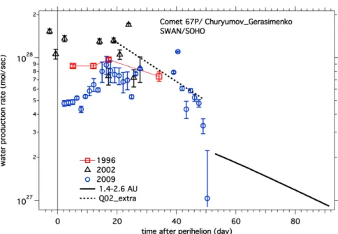
Fig. 1.Water production rates in comet 67P/Churyumov-Gerasimenko. They are derived from Lyman-α single-images collected by SWAN/SOHO
at three last perihelion passages in 1996, 2002, and 2009. The error bars show the formal error resulting from instrument noise and model fitting. The error bars do not include a 30% systematic uncertainty. The change in the level of the production rate near perihelion from 1996 to 2009 is remarkable. However, the activity levels are more similar by 25 days after perihelion. These data are taken from Bertaux et al. (2014). The dashed line is an interpolation between a 2002 point at 18 days after perihelion and a 2009 point at 45 days after perihelion to complement the 2002 SWAN measurements after the last point at 28 days. The solid line is an interpolation between a point at 1.4 AU suggested by SWAN values in 2009 and the Rosina/COPS estimate at 2.6 AU.
over time, as well as some extrapolations that together yielded an estimated total H2O loss rate for the three last orbits of the perihelion passages in 1996, 2002, and 2009. Finally, we take into account the contribution of some other gases (mainly CO and CO2), the gas density measurements of Rosetta (Bieler et al.
2015), and the Rosetta-observed dust-to-gas mass ratio to esti-mate the thickness of esti-material lost at each orbit. In Sect. 3 we discuss the kinematics of the nucleus rotation during two epochs to verify whether the observed outgassing rate is responsible for the observed changes in the rotation period. The first epoch refers to the orbit centered on the perihelion in 2009, where a decrease of the rotation period of 1285 s was measured (Mottola et al. 2014). The other epoch refers to the changes observed since the approach in 2014 until May 2015, which showed a reverse trend: an increase of the rotation period of up to 98 s. For the sake of completion, we also discuss the effect of a possible thermal di-latation on the rotation as well as of the progressive separation of the two lobes of the nucleus of comet 67P.
2. Mass-loss estimates
When comets are within 3–4 AU from the Sun, solar UV pho-tolysis of H2O and then of the OH radical is the main source of atomic hydrogen in the coma, producing a huge envelope that is illuminated through resonance scattering by solar hydro-gen Lyman-α radiation at 121.566 nm that becomes detectable by space-borne Lyman-α photometers, as was first reported for comet Bennett (Bertaux & Blamont 1970). When these observa-tions are compared to appropriate models, it provides a reliable measure of the water production rate and its variation in time in comets, as was done for comet Bennett (Bertaux et al. 1973) and many more comets since. The primary scientific mission of SWAN/SOHO is to determine the latitude distribution of the so-lar wind and its changing pattern during the soso-lar cycle (Bertaux et al. 1995).
An important secondary objective of SWAN is the moni-toring of outgassing of comets. From its viewpoint in a halo orbit around the L1 Lagrange point between the Earth and Sun, at 1.5 × 10⁶ km, SOHO is beyond the geocorona, and the cometary H Lyman α is not impeded by the exospheric Lyman α emission of the terrestrials H atoms, as is the case for observatories that orbit at low altitude, like the Hubble Space Telescope (HST). The usual observation mode of SWAN for monitoring the solar-wind distribution is the mode designed to collect full-sky Lyman-α maps. This means that active comets may be detected in these maps, and this was the case for the 67P apparitions of 1996 and 2002. For interesting comets, a dedi-cated observation campaign was organized in the SWAN pro-gram. This was the case for 46P/Wirtanen near its 1997 perihe-lion (when the comet was still the target of the Rosetta mission) and of 67P around the perihelion in 2009, when it was decided to change the target of Rosetta because of some concerns about the reliability of the Ariane launch rocket before the scheduled launch to 46P/Wirtanen. The SWAN data for 46P/Wirtanen were analyzed with a simple Haser model (Bertaux et al. 1999), while subsequent analyses (including the current data for 67P) to re-trieve Q(H2O) from Lyman-α maps were made with a more so-phisticated model developed by Michael Combi at the University of Michigan that is described in detail in Mäkinen & Combi (2005).
The measurements of Q(H2O) from SWAN are displayed in Fig.1 as a function of time for the three apparitions in 1996, 2002, and 2009 with 4, 10, and 28 measurements, respectively. All observations were collected after perihelion except for two in 2002. The variable error bars are due to interferences from hot stars in the FOV of SWAN, which vary with the position in the sky. In addition, there is an overall uncertainty of about ±30% re-sulting from the typical uncertainties in instrument calibration, model, and model parameters. To extract an estimate for the to-tal H2O sublimation along one full orbit by integrating Q(H2O)
J.-L. Bertaux: The erosion rate of comet 67P Table 1. Gas- and dust-mass ejection per orbit.
Line n Half/full orbit Mass ejected 1996 2002 2009 1 half Period 1.H2O SWAN measurements (kg) 8.59e+08 8.71e+08 8.38e+08
2 half Period 2. H2O complement to 1.4 AU (kg) 1.17e+08 3.57e+08 2.71e+07
3= 1 + 2 half H2O mass from perihelion to 1.4 AU (kg) 9.76e+08 1.23e+09 8.65e+08
4 half Period 3. H2O estimate for 1.4 ≤ Rh ≤ 2.6 AU (kg) 2.37e+08 2.37e+08 2.37e+08
5= 1 + 2 + 4 half Total H2O mass from perihelion to 2.6 AU (kg) 1.21e+09 1.46e+09 1.10e+09
6= 5 × 1.45 half Total gas mass from perihelion to 2.6 AU (kg) 1.76e+09 2.12e+09 1.60e+09 7 half Period 4: gas from COPS for 2.6 ≤ Rh ≤ 3.6 AU (kg) 3.08e+07 3.08e+07 3.08e+07 8 half Period 5: dust measurements for 3.6 ≤ Rh ≤ 4.4 AU (kg) 1.73e+08 1.73e+08 1.73e+08 9= 6 + 7 half Total gas from perihelion to 3.6 AU (kg) 1.79e+09 2.16e+09 1.63e+09 10= 2(2 × 9 + 8) full Total dust hyp 1 Dust/gas = 2 (kg) 7.51e+09 8.97e+09 6.87e+09 11= 2(6 × 9 + 8) full Total dust hyp 2 Dust/gas = 6 (kg) 2.18e+10 2.62e+10 1.99e+10 12= 2(8/2) full Period 5: gas (kg) Hyp 1 Dust/gas = 2 3.6 ≤ Rh ≤ 4.4 AU 1.74e+08 1.74e+08 1.74e+08 13= 2(8/6) full Period 5: gas (kg) Hyp 2 Dust/gas = 6 3.6 ≤ Rh ≤ 4.4 AU 5.8e+07 5.8e+07 5.8e+07 14= 2 × 9 + 12 + 10 full Total mass gas+dust dust hyp 1 (kg) 1.13e+10 1.35e+10 1.03e+10 15= 2 × 9 + 13 + 11 full Total mass gas+dust dust hyp 2 (kg) 2.55e+10 3.06e+10 2.32e+10 16= 14/density full Volume 1 (m3) 2.4e+07 2.86e+07 2.19e+07 17= 15/density full Volume 2 (m3) 5.42e+07 6.51e+07 4.94e+07
18= 16/area full Thickness 1 (m) 0.50 0.60 0.46 19= 17/area full Thickness 2 (m) 1.14 1.37 1.04
20 full Total H2O mass (kg) 2.5–2.6e+9 3.0–3.1e+9 2.3–2.4 e+9
versus time, we assumed that the production is equal before and after perihelion. Then, the post-perihelion period was divided into five time sections.
1. From perihelion to the end of the SWAN measurements. 2. From the end of the SWAN measurements to the time when
a heliocentric distance of 1.4 AU is reached. The production rate decreases seriously at this point.
3. From the time when 1.4 AU is reached to 2.6 AU.
4. From the time when 2.6 AU is reached to 3.6 AU, we rely on the in situ measurements of the total gas density and produc-tion rate of the Rosetta COPS sensor in 2014 (Bieler et al. 2015).
5. Beyond 3.6 AU, we have no estimate of the gas production, but there is an estimate of the dust production rate from the analysis of many comet or coma ground-based images taken in 2007 and 2008 (Snodgrass et al. 2013).
Ejected masses of H2O, dust, and gas are displayed in Table1, where we indicate whether the quantity is estimated over half an orbit or a full orbit. The details of estimates are described below. For period 1, we ignored the two points before perihelion for 2002 and numerically integrated during the period of actual measurements (line 1 of Table 1).
For period 2 and the perihelion in 1996, there are only four SWAN measurement points from 5.1 to 34 days after perihe-lion, at which point the distance to the Sun was 1.362 AU, and a distance of 1.4 AU was reached 45 days after perihelion. We linearly extrapolated the two last points of SWAN between 34 and 45 days after perihelion (line 2 of Table 1).
For period 2 and the perihelion in 2002, there are ten SWAN measurement points, eight of which were taken 2.3 to 28 days af-ter perihelion, at which time the distance to the Sun was 1.33 AU, and a distance of 1.4 AU was reached 45 days after perihelion. To estimate Q(H2O) from 1.33 to 1.4 AU, we interpolated and ex-trapolated logarithmically between the point in 2002 at 1.31 AU and the Q(H2O) value for 2009 at 1.361 AU. The resulting curve is the dashed line in Fig.1, obtained somewhat arbitrarily with mixing the passages in 2002 and 2009 (line 2 of Table 1).
For period 2 and the perihelion in 2009, there are 28 SWAN measurement points taken from 2.2 to 50.3 days after perihelion,
at which time the distance to the Sun was 1.39 AU, and a distance of 1.4 AU was reached 53.5 days after perihelion. We ignored the last SWAN point, which is possibly an outlier on the low side, and added a production rate of 3× 1027mol/s for 3.5 days (line 2 of Table 1).
Line 3 of Table 1 is the H2O production from perihelion to 1.4 AU, the sum of lines 1 and 2 (half orbit).
For period 3, we interpolated (linearly in a log-log plot of Q(H2O) versus the heliocentric distance Rh) between a value of Q(H2O)= 2.1 × 1027 mol/s at a distance of 1.4 AU (as sug-gested by 2009 SWAN measurements) and the actual COPS measurements at 2.6 AU of Q(H2O)= 1 × 1026/1.2, at the end of 2014, as derived inBieler et al.(2015). The division by 1.2 was made to transform COPS measurement of the total density into a production rate of H2O, taking into account 10% of CO2 and 10% of CO. This represents a rough estimate of the aver-age ratios CO2/H2O and CO/H2O as measured by the Rosina mass spectrometer, although these ratios are found to be vari-able, depending on the location of Rosetta w.r.t. the nucleus
(Hässig et al. 2015). The corresponding Q(H2O) is represented
by a solid black line in Fig. 1. For the time integration away from SWAN measurements, we used the actual ephemeris of the comet for all three perihelions (Rh distance versus time) that are found on the Institut de Mécanique Céleste et de Calcul des Ephémérides (IMCCE) server for the ephemeris of solar system objects1.
The total mass production of H2O from perihelion up to 2.6 AU (line 5 of Table1) was computed by summing the productions for the three first periods. The total gas mass ejec-tion (line 6) is obtained by adding 45% to account for 10% CO2 and 10% CO outgassing (as said above). The associated error is estimated to be about 40%.
For period 4 from 2.6 to 3.6 AU, the COPS in situ total gas measurements were transformed byBieler et al.(2015) into a production rate by scaling to sublimation models, taking into ac-count the actual shape of the nucleus, the actual solar illumina-tion, and the expansion of the coma (Bieler et al. 2015). Taken together, COPS data indicate that the production rate was con-stant from early August 2014 (at 3.6 AU) to 1 November 2014 at
1 http://www.imcce.fr/langues/en/
a value Qtotal= 5 × 1025 mol/s, in agreement with the estimate of 4 × 1025 H
2O mol/s at 3.5 AU derived from the MIRO sub-millimeter instrument (Gulkis et al. 2015). After 1 November, COPS data indicate that the production rate doubled and re-mained constant at 1 × 1026 mol/s up to 1 January, 2015, around 2.6 AU. Therefore, we integrated these two total gas pro-duction rates according to these two constant values, yielding a gas mass of 3.08 × 10⁷kg (line 7 of Table 1).
For period 5 beyond 3.6 AU, the analysis ofSnodgrass et al. (2013) indicates a dust content in the coma varying as a power law of the heliocentric distance Rh. The retrieved quantity is Afρ, (where A is the albedo, f is the filling factor, and ρ is the radius of integration in the coma, in cm). Measurements were fitted with single power-law fits pre- and post-perihelion, given by Af ρ= 958 × Rh−3.18(cm) and Af ρ= 1552 × Rh−3.35(cm), respectively.
The quantity Af ρ is (with simple assumptions) proportional to the dust production rate, with a convenient relationship where Af ρ in cm ≈ Qd in kg s−1 (A’Hearn et al. 1995). We used this relationship and integrated in time along the orbit. Snodgrass
et al. (2013) indicated that there was no detectable activity
at 4.4 AU in September 2007. The integration from 3.6 to 4.3 AU yields 1.52 × 10⁸kg and 1.95 × 10⁸kg, respectively, before and after perihelion, with an average of 1.73 × 10⁸kg for a half-orbit (line 8 of Table 1). If the integration is pursued from 4.3 to aphe-lion at 5.68 AU, it would add another 3 × 10⁸kg. But since no activity was recorded beyond 4.3 AU, we preferred not to add this somewhat dubious extrapolation outside of the range where it was established. This dust production (3.6 to 4.4 AU) also cor-responds to some gas production that must be added to the whole mass estimate. Taking a dust-to-gas ratio of 2 or 6 (extreme val-ues considered here, see discussion below), this yields a small extra mass of gas of 1.73 × 10⁸ kg (line 12) or 5.8 × 10⁷ kg (line 13) for a full orbit beyond 3.6 AU.
During period 4 from 2.6 to 3.6 AU, the gas mass as retrieved from COPS is 3.0 × 10⁷kg (line 7 of Table 1). Therefore, the to-tal gas (up to 3.6 AU, still on half-orbit) is obtained by summing lines 6 and 7, to achieve the result presented in line 9.
We now rely on a dust-to-gas ratio to estimate the total ejected mass. From a combined analysis of OSIRIS images of individual grains and of the GIADA dust collector (which col-lects different grain sizes), the dust-to-gas ratio was estimated to be 4 ± 2 (Rotundi et al. 2015). This wide range reflects the fact that the dust mass is dominated by the largest grains, which cut-off size is difficult to determine from photometric measurements of dust (e.g.,Fulle et al. 2004). Since we need an average esti-mate over the full orbit and since we are not sure that the mea-sured ratio at 3.5 AU is valid over the full orbit, we considered two extreme hypotheses to estimate the total mass loss: 2 and 6 for the dust-to-gas ratio, called hypothesis 1 and hypothesis 2, respectively.
Assuming that the loss is symmetrical w.r.t. the perihelion, we may now estimate the total losses of dust for the two dust-to-gas ratio hypotheses, lines 10 and 11, respectively; adding the gas of line 9 and lines 12 or 13 yields the total mass ejected of gas+dust on lines 14 and 15, from 1 to 3 × 10¹⁰kg, depending on assumed dust-to-gas ratio.
This means that a significant fraction of the comet total mass (1013 kg,Pätzold et al. 2015) is lost at each perihelion passage at 1.3 AU: between 0.1 and 0.3 percent. The volume of the lost material (lines 16 and 17 of Table 1) was computed from the measured average density of 470 ± 45 kg/m3 derived from the mass and the total volume of 21.4 ± 2.0 km3 estimated from OSIRIS images (Sierks et al. 2015). Following this, we derived
the thickness of the lost material from the surface of the nucleus, which area was estimated to be 47.4 km2from the shape model of the nucleus (Preusker et al. 2015), as analyzed byJorda et al. (2015). We found values of between 0.50 and 1.37 m (lines 18 and 19 of Table1). The total H2O mass per orbit (line 20) was 2.3 to 3.1 × 10⁹kg, depending on the apparition.
Considering the results of Table 1, one may compute the rela-tive productions rates of H2O within the four orbit sections from perihelion to 1.4 AU, 1.4–2.6 AU, 2.6–3.6 AU, and 3.6–4.6 AU. We found that H2O production is dominant within 1.4 AU, repre-senting 73–76% of the total, the other sections reprerepre-senting 20%, 1.8%, and 1.7 to 5% of the total (according to the assumed dust-to-gas ratio in the outer part of the orbit), respectively. Our SWAN/SOHO measurements of 2009 cover most of the inner section from perihelion to 1.4 AU, and the absolute error is about 30%. The main factors of uncertainty in our estimate of the total mass loss come from the hypothesis of symmetry about perihelion (loss only depends on the distance), and the assumed average dust-to-gas ratio.
Taking the two extreme hypotheses of 4 ± 2 for the dust-to-gas ratio fromRotundi et al.(2015), this wide range probably also includes the other sources of uncertainties that affect the result, which are
− the assumption that the water and dust production rates are symmetric versus the perihelion;
− the assumption that the dust-to-gas ratio is constant over the whole orbit, while we relied on the Rosetta numbers measured at 3.5 AU pre-perihelion (Rotundi et al. 2015). Neither of these two assumptions is consistent with the analy-sis ofFulle et al.(2004), who found (from the analysis of dust brightness mapping at 2002 perihelion passage of 67 P) that the dust production rate was approximately constant within 150 days from perihelion, but at 100 kg/s before perihelion, and 10 kg/s after perihelion, and found the opposite behavior of the gaseous coma observations of OH, CN, C3, C2, and NH during the pas-sage in 1982, with more gas found after perihelion than before
(A’Hearn et al. 1995;Cochran et al. 1992). This would imply
a large decrease of the dust-to-gas ratio in the time before and after perihelion. By assuming a symmetry about perihelion, we might overestimate the gas production (since we mainly con-sidered post-perihelion SWAN H2O data), but we might under-estimate the dust production before perihelion with a constant dust-to-gas ratio. One effect might more or less compensate for the other in estimating the total ejected mass. Notwithstanding some contradictions, and hoping that all systematic effects will not conspire to go in the same direction away from our central estimate, we summarize our results by describing the thickness of the lost layer as 1.0 ± 0.5 m per orbit, which encompasses a range of a factor of 3. Clearly, the situation will be greatly clari-fied after the passage in 2015, when post-perihelion data will be analyzed, and better estimates of the thickness of the lost layer will be possible, hopefully directly by OSIRIS NAC (Narrow Angle Camera) images of terrain changes.
This value of 1.0 ± 0.5 m per orbit is an average over the whole nucleus. It is certainly lower in some areas, and it is cer-tainly more in other areas. Moreover, it is not clear at this point which fraction of the solid material is detached from the nucleus and escapes for ever, and which fraction returns to the ground after each perihelion passage. It is clear that the returned ma-terial constitutes the blanket layer of “smooth” mama-terial seen in many areas. There is some evidence, however, that this layer is not very thick in many areas. For instance, an image of the so-called pits (Fig. 8 inSierks et al. 2015) shows the inside wall of
J.-L. Bertaux: The erosion rate of comet 67P
the pit and its “goosebump features”, while the external part of the pit is covered by a blanket. The thickness of the blanket seen from the side is much thinner than the characteristic scale, ∼3 m, of the goosebumps.
In most parts of the comet, the whole smooth blanket is therefore probably completely blown out at each perihelion, with a only small fraction falling back on the ground. This would prevent the formation of a solid crust, which has sometimes been invoked to describe the surface of the nucleus. One ex-ception might be the smooth terrain in the region of the neck, denominated the Hapi region (Thomas et al. 2015), which is not illuminated closer to the Sun, as pointed out by the referee.
Keller et al.(2015a) have also addressed the question of ero-sion of comet 67P in a totally different way. They used the ac-tual shape of the nucleus described by more than 105 facets, and a “simple” ice sublimation model, considering three cases: dirty ice directly exposed to the Sun (model A), or covered by a porous dust layer of 50 µm (model B) or 1 mm (model C). They concluded that only a small fraction of the surface nu-cleus is active (but spread everywhere like on a chess board). There is also a large difference of erosion between the north part (erosion around 1 m or slightly below), while the southern hemi-sphere, which is fully exposed near perihelion, would experience more than 4 m, reaching 10 m at some places. They found water mass losses for models A, B, C of 6.5 × 10¹⁰ kg, 4.9 × 10¹⁰kg, and 1.5 × 10¹⁰ kg, respectively, and an ejected material layer thickness of 14.5, 11, and 3.4 m. This is more than our esti-mates, which is based on actual H2O outgassing measurements. The authors checked that their model predicts a higher H2O out-gassing rate than observed by SWAN at perihelion (factor of 16 for their favorite model B), meaning probably that only 6% of the southern hemisphere surface is active, as described by their model.
We may compare our result for 67P to erosion studies per-formed on two other comets that have been encountered by space missions, for which the size of the nucleus and its area were also determined. For comet 9P/Tempel 1, a loss of ≈1/3 m per orbit or ≈3 × 10⁻⁴of the total mass per orbit was already mentioned
(Thomas et al. 2013b). For comet 103P/Hartley 2, this was 3%
of the total mass of the nucleus, and 1% in 2010 (Thomas et al.
2013a). Therefore, at a loss rate of 0.1–0.3% mass per orbit,
comet 67P is in between these two cases on a log scale. We note that for the three comets that have been visited by space missions, the estimate of the lost layer thickness varies over a smaller range (from 1/3 m to 4.4 m per orbit, about one order of magnitude range), while the loss of relative mass per orbit ranges over two orders of magnitude.
On the other hand,Groussin & Lamy(2003) have estimated the erosion rate for comet 46P/Wirtanen to be 0.5 m per orbit. They used a radius of the comet of 0.6 km derived from HST ob-servations, and their surface activity model was also adjusted to the observed perihelion production rates of H2O. This value is quite comparable to our value found for comet 67P, but it also implies a much greater relative mass loss because the comet is smaller.
Since the encounter with Jupiter in 1959, comet 67 P passed only eight times through its perihelion. Given our erosion rate of 1 m per orbit, this would correspond to a cumulated erosion of only 8 m thickness.
Orbital simulations of comet 67P backward in time
(Groussin et al. 2007) showed that before 1959, the
peri-helion distance was larger than 2.7 AU for a duration of about 400 years, implying little erosion and little geological evo-lution of the nucleus. At this time (around year 1597), there
was a close planetary encounter with a broad variety of possi-ble scenarios before that encounter (chaotic behavior). Some of them include periods of time when the comet had a perihelion around 1 AU, while others have an orbit with large perihelions, and therefore little erosion. Therefore, if some features observed now imply an erosion much stronger than 8 ± 4 m, it would mean that the former scenarios (with small perihelions) are fa-vored. We present an example of such an interpretation, admit-tedly highly speculative at this time. There are a number of circu-lar features (Fig. 9 ofAuger et al. 2015) that we could interpret as being the remnants of ancient pits, similar to the numerous circular pits detected (Sierks et al. 2015;Vincent et al. 2015) on the nucleus. The material infalling in the bottom of the pit would remain there and could form some consolidated material. When the erosion would peel off the nucleus around the pit down to the bottom of the pit (or even below), it would remain a circular fea-ture similar to those observed.Vincent et al.(2015) showed that some pits have a depth of up to 20–200 m, which is much larger than the erosion since 1959. Therefore, if the observed circular features are shown to be remnant bottoms of ancient pits, this would be a strong indication of substantial erosion before 1959, favoring the scenarios before 1597 in which comet 67P experi-enced a period of its orbital lifetime in the inner solar system, with a perihelion distance to the Sun much smaller than 2.7 AU, rather than other scenarios where the comet perihelion was al-ways larger than 2–3 AU. Another important result of the sim-ulations ofGroussin et al. (2007) is the dynamical lifetime of comet 67P, which is estimated to be about 105 000 yr.
We now investigate the role of the material ejection in the observed changes in the spin rate of the nucleus.
3. Kinematics of the nucleus rotation
3.1. Observations
The rotation of the nucleus of 67P is mainly a pure rotation around the axis of maximum inertia (Sierks et al. 2015). In Table2we list the epochs, periods, rotation rates and changes in rotation rates that are discussed for comet 67P. Epoch 5 for 26 May, 2015 was added during the revision process of this paper with new available data, and the discussion was updated accordingly. Here we consider the measured changes in rota-tion rate both during approach and escort phase (August 2014 to May 2015, epochs 3 to 5 of Table2, Fig.2) and the change be-tween 2004–2007 (before 2009 perihelion, epoch 1) and well af-ter the 2009 perihelion, during the 2014 approach phase (Mottola
et al. 2014). During this approach phase (in the period 23
March to 24 June, 2014, epoch 2), while the nucleus was still unresolved in the OSIRIS NAC, a time series of photometric measurements allowed accurately pinpointing a sidereal rota-tion period of 12.4043 h (Mottola et al. 2014) or 12 h 24 mn 15.48 s corresponding to a rotation rate ω= 0.000140704 rad/s (Table 2). This period was significantly shorter (by 1285 s) than the one determined from ESO NTT ground-based ob-servations at large distance from the Sun in the period from February 2004 to September 2007 (epoch 1 of Table2), well before the perihelion in 2009 (Lowry et al. 2012): Psid = 12.76137 ± 0.00006 h. This decrease in period most certainly occurred around the perihelion passage in 2009, most probably forced by sublimation-induced torques.
On the other hand, the combination of NAVCAM images, tracking of Rosetta, and some OSIRIS images has allowed the ESOC Rosetta navigation team to measure the rotation pe-riod of the nucleus of 67P and its change since the beginning
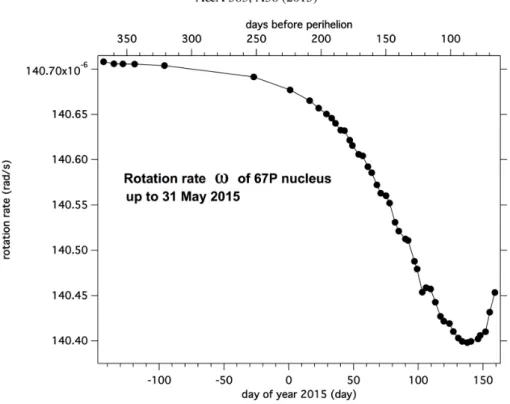
Fig. 2.Variations of the rotation rate measured since the rendezvous of Rosetta with comet 67P up to 8 June 2015. These data were obtained by the ESA navigation team at ESOC through a refined analysis of many landmarks on the nucleus observed by the ESA navigation camera NAVCAM. Bottom scale: day of year 2015. Top scale: days before 2015 perihelion. The perihelion is on August 13, 2015, or day 225.
Table 2. Rotation rates of the nucleus of 67P.
Epoch number Epoch of measurement Period Psid Rotation rate ω Change in rotation rate∆ω
decimal hours 10−4rad/s 10−6rad/s
1 2003–2007 12.76137 ± 0.00006 1.36767 NA 2 March to June 2014 12.4043 ± 0.00007 1.40704 +3.94 3 1 August to 6 Oct. 2014 12.4041 ± 0.02 s 1.40706 Not significant 4 23 February 2015 12.4129 ± 0.1 s 1.40606 –0.100 5 17 May 2015 12.4309 ±0.1 s 1.40402 –0.304
of the escort phase (rendezvous with the comet was achieved on 7 August 2014). Their data, extracted from their VSTP reports that are included in the Rosetta Mission Operation Reports, are plotted in Fig.2. Since the analysis of Osiris pho-tometric observations while the nucleus was still unresolved in March-June 2014, the rotation period has increased by 32 s up to the end of February 2015, and 98 s up to 17 May 2015.
This recent behavior of decreasing rotation rate is the inverse of what occurred during the perihelion passage in 2009. Before discussing the implications, we recall a few kinematics equa-tions governing the laws of the change in the angular momentum of a rotating body (boldface indicates vectors), as schematically illustrated in Fig.3:
d(Iω)
dt =
Z
rXd f, (1)
in which I is the moment of inertia of the nucleus, ω is the ro-tation rate (in radians/s) = 2π/P (P period in s), r is one vec-tor joining the center of mass of the nucleus to one point of its surface at distance r, d f is the elementary force exerted by out-gassing from the surface, X is the vectorial product, and the in-tegral is made over the whole surface of the nucleus. According
toMottola et al.(2014), there are very few observed changes in
the rotation period of comets, and (to the best of our knowledge)
they were all interpreted with the moment of inertia being kept fixed. In this case, Eq. (1) becomes
Idω dt =
Z
rXd f. (2)
Here we first keep the possibility to change the moment of in-ertia. This is motivated by the two-lobe structure of the nucleus of 67P, the presence of a crevice in the neck (Hapi region), and the possible increase of the distance between the two lobes as a sign of separation. There is also the case of thermal dilatation, which would increase the moment of inertia.
For a spherical nucleus, there is a rotation rate ωLfor which the centrifugal force is equal to the gravity at equator, which is independent of the radius,
ωL= r
4πρG
3 , (3)
where ρ is the density and G is the gravitational constant. Taking ρ = 470 kg/m3gives ω
L = 3.62 × 10⁻⁴rad/s, corresponding to a period slightly shorter than five hours. It is likely that a rotation faster than the limit ωLwill result in a disruption of the comet nu-cleus. Indeed, in his review of known periods of comets (deter-mined at that time by regular patterns in the coma assigned to the
J.-L. Bertaux: The erosion rate of comet 67P
rotation of the nucleus),Whipple (1982) did not find any comet with a faster rotation among 47 comets for which a rotation pe-riod could be measured. More recently,Weissman et al.(2004) derived a more sophisticated formula than our spherical case of Eq. (3) for the case of an oblate nucleus. The oblateness may be obtained from carefully analyzing the light curve of the bare nu-cleus. They found that the shortest period of the 14-comet sam-ple available (oblateness and rotation) was 5.6 h, just above the limiting value ωL = 5 h for a spherical nucleus at 470 kg/m3. If the same decrease of rotation rate (as in 2009) is experienced at each perihelion of comet 67P, the limit ωLwill be reached in 56 orbits, around year 2375.
Going back in time, the rotation rate would have been 0 only 35 orbits in the past, but nothing would preclude that the rotation would reverse its sense with the same exerted torques. However, the extrapolation of the orbit back in time cannot be made accurately before 1959, when a close encounter with Jupiter was experienced, and before this, the perihelion distance was much larger and the corresponding torque smaller (Groussin et al. 2007).
3.2. Case without torque
In a first approach, we ignore the effect of torques and exam-ine the observed changes of the rotation rate between epochs 1 and 2, then between epochs 3 and 4 or epoch 5 (Table 2). Between two epochs, the change in rotation rate ∆ω and the change in momentum of inertia∆ I are related by
∆ω ω +
∆I
I = 0. (4)
We consider two phenomena that could induce a change in the moment of inertia I. These are thermal dilatation of the nu-cleus associated with the thermal wave penetrating the nunu-cleus while the comet is approaching its perihelion, and the other is an increase of the distance between the two lobes of 67P. Form epoch 1 to epoch 2 (before and after perihelion in 2009, respec-tively) the angular velocity increased by 3.94 × 10⁻⁶ rad/s (the period increased by 21.4 mn). Since the dilatation is connected to the thermal wave, it should be roughly symmetric around per-ihelion, with a retraction after perihelion. Therefore we do not expect the velocity increase to be due to this phenomenon. And since an increase of the rotation rate ω is seen, it should induce (Eq. (3)) a decrease of I, while the separation of lobes would induce an increase of the moment of inertia. Therefore, the ob-served increase of ω is most likely connected to the torque ex-erted by outgassing of the nucleus. The situation is different from epoch 3 to epochs 4 and 5 while Rosetta was in the vicinity of the nucleus. The angular velocity was seen to decrease and therefore could be the sign of either thermal dilatation or separation of the two lobes.
Separation of the lobes:considering the masses of the two lobes M1 = αM and M2= (1−α)M, with M being the total mass and a = a1+ a2the distance between the two lobes, the sum of the distances a1and a2 of the center of gravity of each lobe to the center of gravity of the nucleus. The moment of inertia I can be described as
I= a21M1+ a22M2= a2Mα(1 − α). (5)
Therefore, combining Eqs. (4) and (5), we have the relationship da a = − 1 2 dω ω · (6)
According to Jorda et al. (2015), a = 2600 m, yield-ing da= 0.92 m for epoch 4 and 2.8 m for epoch 5. This increase in separation could be confirmed (or refuted) by a care-ful analysis of landmarks on both lobes.
Thermal dilatation: the evolution of the spin rate of comet 9P/Tempel over two perihelion passages was determined and discussed thoroughly byBelton et al.(2011). They found that the period decreased by 16.8 ± 0.3 min during the pas-sage in 2000 and by 13.7 ± 0.2 min during the paspas-sage in 2005, suggesting a secular decrease in the net torque. These authors considered only the torque from outgassing. In addition to the main effect at perihelion, they also found a small deceleration before perihelion and a symmetrical acceleration after the per-ihelion. This somewhat mimics what can be expected from the effect of thermal dilatation or retraction (their Fig. 22), and it was tempting to also try this hypothesis with comet 67P.
For a homogeneous sphere, the moment of inertia is I = 2/5 M R2. An increase in length∆ L due to thermal expansion with an increase in temperature∆ T is ∆L = Lβ∆ T. The thermal dilatation coefficient β of a comet is totally unknown for the time being. As a guide, β= 12 × 10−6/K for steel, β = 50 × 10−6/K for water ice, and may reach 150 × 10−6/K for synthetic or-ganic materials like Rilsan. If the whole comet were inflating homogeneously, we would have the relation
∆I I = 2 ∆R R = 2β∆T = − ∆ω ω · (7)
Since we observe between epochs 3 and 4 dωω = −7 × 10⁻⁴, with β = 100 × 10−6it would require a modest increase of the internal temperature∆T = 2.1 K, or 18 K if β = 12 × 10−6/K. The radius R= 2000 m of the comet would have increased by 0.42 m in both cases between epochs 3 and 4 and by 1.3 m between epochs 3 and 5. But the actual situation is more complicated, since only an outside layer of the comet sees a change in temperature along its orbit. As discussed inMcKay et al.(1986), one may define a depth below which the temperature is constant throughout the or-bit. The thermal skin depth should be about 7 m for comet 67/P, and therefore only the dilatation of this external part could in-crease the moment of inertia. Indeed, if only the skin is affected by dilatation, it is found that the skin would have to move out-ward by about 30 m to change the inertia enough to induce the observed change in ω between epochs 3 and 4, which is absurd, and would certainly have been noticed in the navigation analysis of NAVCAM images. Distinguishing between the two options (separation between the lobes, and global thermal inflation) is probably possible by separately examining the inflation of both the body and the head, and of the total nucleus.
3.3. Torque effect of outgassing
Now we ignore the changes in the shape of the nucleus (dilata-tion or separa(dilata-tion of the lobes) and only consider the effect of outgassing as exerting a torque on the nucleus, that can change the rotation state. The moment of inertia I is kept constant, and Eq. (2) applies. This equation can be integrated over time to relate a change in the rotation rate ∆ω during two epochs Ei and Ejto an integrated flux of ejected material during the same time. In this section we wish only to evaluate orders of mag-nitude, and some approximations are justified. The moment of inertia I is approximated as the one for a homogeneous sphere of radius R, I = 2/5 M R2. The force exerted by outgassing is f = Vdm/dt, where dm/dt is the mass ejection rate, and V is the velocity vector of ejection. The magnitude of the torque R X f is
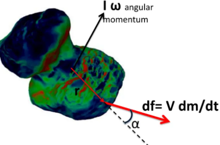
Fig. 3. Schematic representation of the torque exerted on the nucleus by the outgassing. The flow of gas V from one point makes an angle α with the line joining the center of mass of the nucleus and the point of outgassing.
RV sin α dm/dt, where α is the angle between the radius vector R and the velocity V. It is generally assumed that the gas velocity is perpendicular to the local surface, but the expression is cor-rect even if this assumption is not fulfilled. For simplicity we here only consider the component of the torque aligned with the angular momentum, which affects the rotation rate. Assuming a certain pattern of the outgassing (integrated over one rotation) to be stable over some time between epochs Eiand Ej, the geo-metrical part of the integral of Eq. (1) can be separated from the time integral of dm/dt, and Eq. (1) may be rewritten as
Vhsin αi Z E j
Ei
Qdt= 2
5MR∆ω, (8)
where hsin αi is an average value of sin α over the nucleus. The angle α and its sine may be either positive or negative, increas-ing or decreasincreas-ing the rotation rate, respectively. From Eq. (8) an estimate of hsin αi may be computed by placing numbers in the other terms that are known or estimated. For instance, if we were to find hsin αi larger than 1, this would demonstrate that the torque forces are insufficient to explain the observed change in rotation rate.
Only the gas production rate must be taken into account in the integral of Q over time. This is because the solid material that is lifted off from the surface of the nucleus takes its energy and momentum from the gas drag. For an estimate of V, we rely on the detailed study ofDavidsson et al.(2004) of the force exerted on a porous cometary material outgassing water vapor. In the frame of their layer energy absorption model (LEAM) that con-siders the ice sublimation inside a porous material, they com-puted that a force F of 0.18 newton per unit surface element would be exerted by a gas flow of Z = 2.5 × 10⁻⁴ kg m−2s−1 (their Figs. 11 and 12 at maximum temperature). Therefore, their estimate of hVi is derived from F = ZhVi, which yields hVi = 720 m/s. Another approach (Zakharov, priv. comm.) would be to take the average of the thermal velocity components in the normal-direction averaged over only those molecules moving in the positive normal-direction: sqrt(2kT/πmH2O) (which is one half of the averaged thermal speed), yielding 260 m/s for T = 230 K. In view of the actual Doppler velocity measurement of H2O line obtained by MIRO (Gulkis et al. 2015) of 680 m/s, we prefer to consider the 720 m/s value.
We may now derive hsin αi from (8), with M = 1013 kg, R = 2000 m, observed ∆ω from Table2, and an estimate of the
integral of Q dt between two epochs. Between epochs 3 and 4 the length of period is 156 days. With an average production rate of Q(H2O)= 1026mol/s (or 3 kg/s) and hVi = 720 m/s, we find hsin αi = −1.7 × 10⁻², a quite reasonable number. The corre-sponding angle is 0.95◦. The minus sign indicates that the torque is exerted against the existing angular momentum, yielding a de-crease in the spin rate. If the nucleus were perfectly spherical and the outgassing perpendicular to the surface, α would be 0 and the torque would also be 0. But in view of the complicated shape of the nucleus (Sierks et al. 2015;Thomas et al. 2015), the direction perpendicular to the surface is rarely coincident with a direction toward the center of mass, therefore the angle α is often as large as several tens of degrees.
It is nonetheless quite striking that a modest production rate of 3 kg/s thrown almost vertically can still slow the ro-tation of a body of 10 billion tons in a measurable amount. Between epochs 1 and 2, which encompass the perihelion pas-sage in 2009, our estimated gas production (line 9 × 2 for a full orbit+line 12 of Table 1) is approximately 3.5 × 10⁹ kg; in this case, we find hsin αi = +1.2 × 10⁻², and a corresponding angle 0.7◦. This number is quite similar to the number derived from epochs 3 to 4, although it is of opposite sign. This change of sign is most likely linked to the geometry of the outgassing, dic-tated by a combination of the particular shape of the nucleus, the inclination of the rotation axis on the orbital plane, and the so-lar latitude around perihelion. While during the observations of epochs 3 to 5, the northern region was illuminated by the Sun and the southern region was not, the situation is different when inte-grated over a whole orbit. The Sun rapidly crossed the equator of the comet in May 2015 and will reach a maximum southern lati-tude of –52◦three weeks after perihelion. On 28 February 2015, we wrote: “Therefore, if the 2009 outgassing scenario repeats it-self in 2015, we may expect that the rotation of the nucleus is going to continue to slow down for a while after February 2015, but then this slow down will stop when the Sun will explore more southern latitudes, the torque will reverse, and an acceler-ation will take place with a net result on the rotacceler-ation rate change along one orbit similar to the one observed over the last orbit”. With new measurements of the rotation rate provided by the ESOC Flight Dynamics team, Fig. 2was updated with data up to 8 June 2015. The time derivative of the measured rotation rate is also very informative. It is expressed as being proportional to the outgassing rate Q(t) and hsin αi, as shown in Eq. (9) derived from (8): dω dt = 5 2 V MRhsin αiQ(t). (9)
The rotation rate data of Fig.2 was numerically time-derived to obtain the acceleration of Fig.4. This acceleration shows a complex structure with strong periodic oscillations and six well-defined peaks: the first one in 2015 doy 41.6 (10 February), the last one in 2015 doy 121.8 (1 May). The period of the oscillation is determined with the time lapse of 80.27 days between the first and the last peak, yielding a period of 16.05 ± 0.15 days. We do not believe that these oscillations of dω/dt are caused by oscil-lations of Q(t) or osciloscil-lations of hsin αi; for the time being, we interpret these oscillations as linked to the existence of a preces-sion of the spin axis with this particular period, and we suspect that these oscillations are not real, but rather an artifact. The op-tical measurements of the NAVCAM camera could introduce a periodic artifact because the retrieval method of the rotation rate from images is by comparison with a model that probably does not include a precession. In fact, when the strong oscillations are smoothed out (by averaging in a box car of 32 days= two
J.-L. Bertaux: The erosion rate of comet 67P
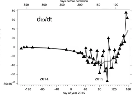
Fig. 4. Black triangles: deceleration of the spin rate since rendezvous with comet 67 P as a function of time from August 2014 to 6 May 2015. Bottom scale: day of year 2015. Top scale: days before 2015 perihelion. They were time-derived from ESOC data of Fig. 2, tained by the ESOC navigation team from the fit of ob-served landmarks with a shape model and an assumed constant spin rate over a period of a few days. The strong oscillations with a period of 16 days are most likely not real and linked to the simplifying assump-tion of no precession (see text). The thick gray line is a smoothed average over 32 days. It shows that the spin rate change went through a minimum around April 10 and changed sign around mid-May 2015, a sign of out-gassing pattern change linked to the solar illumination geometry change, passing to more southern latitudes.
periods) in Fig.4(thick gray line), we see that the acceleration went through a negative minimum around doy 80 (21 March, 2015) and then began to increase. The absolute value decreased (approaching 0 value), meaning that the torque decreased after 21 March. This is certainly not because of a decrease of Q(t) in this pre-perihelion period, but rather the absolute value of hsin αi which decreased, indicating a change in the configuration of the jet system. Therefore, we believe that a new jet system in the south began to operate around this time (and/or an active sys-tem became less active in the north). The reversal of torque that we predicted in our first version of this paper actually occurred on 17 May (smoothed curve in Fig.4), when the acceleration of the rotation rate became positive, which is what was experienced on average over the apparition of comet 67P in 2009. The rota-tion rate has reached a minimum around 21 March, 2015 and it is likely to remain a record low compared to the future.
4. Conclusions and perspectives
We have estimated the total mass of water outgassed at each of the three last perihelions of comet 67P. Taking into account some information collected during the early escort phase from Rosetta instruments (outgassing rate, contribution of CO and CO2, dust-to-gas ratio, mean density, and total area of the nucleus), we were able to estimate the erosion rate per orbit in the present epoch, quantified by the thickness of the layer of lost material: about 1.0 m, within ±50%. This is an important parameter that must be taken into account for the interpretation of the numer-ous features that are observed at the surface of this fascinating comet. In particular, the erosion rate per orbit (0.1 to 0.3% of the total mass) is significant. The comet is peeling off at each or-bit, supporting the idea that the composition of the material that is measured in the coma (gas and solid) is representative of the bulk material of the nucleus.
We have considered three potential mechanisms for a change in the rotation rate of the nucleus in two circumstances. The mechanisms are thermal dilatation, progressive separation of the two lobes, and the more classical outgassing-induced torque. The two circumstances are the changes associated with the per-ihelion orbit in 2009, and the approach in 2014 to early 2015, which is well documented by Rosetta ESOC measurements and analysis. For the perihelion orbit in 2009, gradual separation
of the two lobes is excluded since it would have induced a slower rotation rate, while a higher rate was observed. Thermal dilatation is also excluded for this perihelion orbit, since this is a reversible phenomenon around perihelion, unless orbital changes would induce a complex history of the internal temper-ature profile, with a net cooling during the present orbit with perihelion at 1.3 AU. It would mean that in the recent past the orbit was nearer to the Sun than it is now. This contradicts the fact that before the encounter with Jupiter in 1959, the perihelion distance was larger at 2.7 AU. In contrast, we computed that an outgassing-induced torque is a plausible hypothesis in view of our previous SWAN/SOHO measurements of outgassing. The observed increase in the spin rate indicates that the net average angle α of outgassing is a modest 0.7◦. We calculated that the maximum spin rate ωL would be reached in 56 orbits around year 2375, meaning a rapid disruption of the nucleus at this time. During the approach to perihelion in 2014 to early 2015, Rosetta accurately measured an increase in the period of 32 s up to 23 February, and 98 s up to 17 May, 2015. The implications were explored for the three mechanisms. A gradual separation of the two lobes by 0.92 m and 2.8 m for 23 February and 17 May, respectively, could explain the observed change in spin rate. A global inflation of 0.42 m and 1.3 m, respectively, of the nucleus could also explain the observation. However, if thermal dilata-tion were the cause, it would have to affect the whole nucleus, which contradicts what we understand of the thermal regime inside the nucleus. One could explore the stretching influence of the solar tide, but this is beyond the scope of this paper. A sublimation-induced torque is the most plausible explanation, requiring an average angle of α = 0.95◦, similar (but opposite in sign) to the one required for the integrated orbit in 2009. The change of sign can be explained by insolation geometry.
In addition, the refined analysis performed by ESOC Flight Dynamics team of Rosetta NAVCAM images (based on land-marks) allowed accurately measuring the decrease in the spin rate (Fig.2). At end of February 2015, the spin rate decreased rather fast. We estimate that this fast decrease is difficult to ex-plain with the mechanisms of thermal dilatation. If it is con-nected with the separation of the two lobes, it will soon be detectable in the refined analysis images, the distance between head and body landmarks should increase more than the dis-tance between landmarks on the same lobe. In the case of the
most likely mechanism (outgassing), we wish to emphasize the importance of the spin rate change measurements. They provide a global picture of the activity of the comet, integrated over the whole nucleus and over a few days, which is not attainable by any other Rosetta measurements at present. This quantification of the activity is relative and not absolute for the time being. It is valid as long as the insolation geometry does not change sig-nificantly. To make it absolute, one would have to compare the various activity estimates from the various instruments to this spin rate deceleration.
We have indeed seen around 17 May, 2015 the reversal of torque that we predicted in our first version of this paper, which was written in February 2015. The acceleration of the rota-tion rate became positive and very likely will stay positive after early June, in conformity with the effect of the jet activity aver-aged over a full orbit, as was determined over the apparition of comet 67P in 2009 (Mottola et al. 2014).
Acknowledgements. SOHO is an international cooperative mission between ESA and NASA. Rosetta is an ESA mission. This work is being supported by CNES (Centre National des Études Spatiales) and CNRS (Centre National de la Recherche Scientifique) and its Institut National des Sciences de l’Univers (INSU). We are grateful to many colleagues involved in the Rosetta mission, in particular Uwe Keller, Bjorn Davidsson, Laurent Jorda, Cesare Barbieri, and Vladimir Zacharov for fruitful discussions. We wish to thank Andre Bieler and Kathrin Altwegg for communicating production rates from the COPS/Rosina instrument. We are also very much indebted to Andrea Accomazzo and the Flight Dynamics ESA Navigation Team of Rosetta project at ESOC (Vicente Companys, Mathias Lauer, Frank Budnik, Bernard Godard, Pablo Munoz, Vishnu Janarthanan), for making available to the Instrument Science Teams their estimate of the rotation rate within a few days of their careful analysis.
Note added in proof.Keller et al. (2015b) have made a study parallel to ours on the rotation rate changes of this comet through sublimation activity, with the actual shape model of the nucleus. They reached the following interesting conclusions: 1. The par-ticular shape of the nucleus, combined with the 52◦ inclination of the rotation axis, explains the succession of first a decrease in the rotation rate, then a strong acceleration, as observed. 2. The computed torques with a uniform sublimation efficiency are too large by a factor 5.7 for the period of acceleration (near perihe-lion), consistent with the fact that their model predicts more H2O
outgassing than observed. However, the discrepancy factor is not the same for the two periods, slowing and acceleration, which might indicate an asymmetry of the H2O outgassing properties of the nucleus.
References
A’Hearn, M. F., Millis, R. C., Schleicher, D. O., Osip, D. J., & Birch, P. V. 1995,
Icarus, 118, 223
Auger, A.-T., Groussin, O., Jorda, L., et al. 2015,A&A, 583, A35
Belton, M. J. S., Meech, K. J., Chesley, S., et al. 2011,Icarus, 213, 345
Bertaux, J. L., & Blamont, J. E. 1970,C. R. Acad. Sci. Paris Ser. B, 270, 1981
Bertaux, J. L., Blamont, J. E., & Festou, M. 1973,A&A, 25, 415
Bertaux, J. L., Kyrölä, E., Quémerais, E., et al. 1995,Sol. Phys., 162, 403
Bertaux, J. L., Costa, J., Mäkinen, T., et al. 1999,Planet. Space Sci., 47, 725
Bertaux, J. L., Combi, M. R., Quémerais, E., & Schmidt, W. 2014,Planet. Space Sci., 91, 14
Bieler, A., Altwegg, K., Balsiger, H., et al. 2015,A&A, 583, A7
Cochran, A. L., Barker, E. S., Ramseyer, T. F., & Storrs, A. D. 1992,Icarus, 98, 151
Combi, M. R., Lee, Y., Patel, T. S., et al. 2011a,AJ, 141, 128
Combi, M. R., Bertaux, J.-L., Quémerais, E., Ferron, S., & Mäkinen, J. T. T. 2011b,ApJ, 734, L6
Davidsson, B. J. R., & Skorov, Y. V. 2004,Icarus, 168, 163
Fulle, M., Barbieri, C., Cremonese, G., et al. 2004,A&A, 422, 357
Groussin, O., & Lamy, P. 2003,A&A, 412, 879
Groussin, O., Hahn, G., Lamy, P. L., Gonczi, R., & Valsecchi, G. B. 2007,
MNRAS, 376, 1399
Gulkis, S., Allen, M., von Allmen, P., et al. 2015,Science, 347, 0709
Hässig, M., Altwegg, K., Balsiger, H., et al. 2015,Science, 347, aaa0276
Jorda, L., Gaskell, R., Capanna, C., et al. 2015, Icarus, in press Keller, H. U., Mottola, S., Davidsson, B., et al. 2015a,A&A, 583, A34
Keller, H. U., Mottola, S., Skorov, Y., & Jorda, L. 2015b,A&A, 579, L5
Lowry S., Duddy, S. R., Rozitis, B., et al. 2012,A&A, 548, A12
Mäkinen, J. T. T., & Combi, M. R. 2005,Icarus, 177, 217
McKay, C. P., Squyres, S. W., & Reynolds, R. T. 1986,Icarus, 66, 625
Mottola, S., Lowry, S., Snodgrass, C., et al. 2014,A&A, 569, L2
Pätzold, M., Andert, T., Hahn, M., et al. 2015, Nature, submitted Rotundi, A., Sierks, H., Della Corte, V., et al. 2015,Science, 347, aaa3905
Preusker, F., Scholten, F., Matz, K.-D., et al. 2015,A&A, 583, A33
Sierks, H., Barbieri, C., Lamy, P. L., et al. 2015,Science, 347, aaa1044
Snodgrass, C., Tubiana, C., Bramich, D. M., et al. 2013,A&A, 557, A33
Thomas, P. C., A’Hearn, M. F., Veverka, J., et al. 2013a,Icarus, 222, 550
Thomas, P., A’Hearn, M., Belton, M. J. S., et al. 2013b,Icarus, 222, 453
Thomas, N., Sierks, H., Barbieri, C., et al. 2015,Science, 347, aaa0440
Vincent, J.-B., Bodewits, D., & Besse, S. 2015,Nature, 523, 63
Weissman, P. R., Asphaug, E., & Lowry, S. C. 2004,Comets II, 337
Whipple, F. L. 1982, in: Comets (Tucson, AZ: University of Arizona Press), 227