Counting moving people by staring at a blank wall

Counting Moving People by Staring at a Blank Wall

Prafull Sharma

B.S. in Computer Science, Stanford University (2017)

Submitted to the Department of Electrical Engineering and Computer Science in partial fulfillment of the requirements for the degree of

Master of Science at the

MASSACHUSETTS INSTITUTE OF TECHNOLOGY

June 2019

@

Signature redacted

A u th o r ... ...

Department of Electrical Engineering and Computer Science

May 23, 2019

1

Signature redacted

C ertified by ... e ...

William T. Freeman Thomas and Gerd Perkins Professor of Electrical Engineering and Computer Science Thesis Spervisor

Signature redacted

C ertified by ... ...

Fr6do Durand Professor of Electrical Engineering and Computer Science Thesis Supervisor

Accepted by ...

MASSAHUSETS NSTITUTE _{OFTECNLG Pr}

JUN 13 2019

Signature redacted

j L-/ U Leslie A. Kolodziejski

ofessor of Electrical Engineering and Computer Science Chair, Department Committee on Graduate Students

Counting Moving People by Staring at a Blank Wall

by

Prafull Sharma

Submitted to the Department of Electrical Engineering and Computer Science on May 24, 2019, in partial fulfillment of the

requirements for the degree of Master of Science

Abstract

We present a passive non-line-of-sight imaging method that seeks to count hidden moving people from the observation of a uniform receiver such as a blank wall. The technique amplifies imperceptible changes in indirect illumination in videos to reveal a signal that is strongly correlated with the activity taking place in the hidden part of a scene. We use this signal to predict from a video of a blank wall whether moving persons are present, and to estimate their number. To this end, we train a neural network using data collected under a variety of viewing scenarios. We find good overall accuracy in predicting whether the room is occupied by zero, one or two persons, and analyze the generalization and robustness of our method with both real and synthetic data.

Thesis Supervisor: William T. Freeman

Title: Thomas and Gerd Perkins Professor of Electrical Engineering and Computer Science

Thesis Supervisor: Fr6do Durand

Acknowledgments

I would like to first thank my advisors, Prof. William T. Freeman and Prof. Fr6do

Durand. They have provided constant guidance throughout my thesis. Thanks to them for proposing the idea presented in this thesis and supporting me through the numerous failed attempts at solving this problem. I am grateful for having them by my side.

Thanks to Prof. Gregory W. Wornell, Prof. Antonio Torralba, Prof. Yoav Y. Schechner, Prof. Jeffrey H. Shapiro, Prof. Vivek Goyal, Dr. Franco N.C. Wong for helpful discussions and questions which enabled me to think about the problem from different perspectives.

I have been fortunate to work with Dr. Miika Aittala on this project. Numerous

insights during our discussions have not only shaped the trajectory of this thesis, but also have positively impacted my way of approaching research.

I am grateful to be a part of the vision and graphics community at CSAIL. It

has been a fun learning experience to interact with members of the group. I would like to especially thank (in no particular order), Dr. Katie Bouman, Dr. Micha81 Gharbi, Dr. Zoya Bylinskii, Dr. Tzu-Mao Li, Dr. Ronnachai Jaroensri, Luke Ander-son, Lukas Murmann, Amy Zhao, Yuanming Hu, Camille Biscarrat, Caroline Chan, Spandan Madan, Dr. Jun-Yan Zhu, Dr. Guha Balakrishnan, Jiajun Wu, Xiuming Zhang, Zhoutong Zhang, Vickie Ye, Adam Yedidia, David Bau, among many others. Thanks to the CSAIL administrators, staff at TIG, and CSAIL staff for making

CSAIL an amazing space for conducting research.

Thanks to Harshvardhan, Puneet Jain, and Abhijit Bhadra for contributing to the data collection related to this project and also supporting me otherwise. I would also like to thank all my friends at MIT and outside for injecting the required dose of fun in my life.

I would like to express my gratitude towards my grandmother, mother, aunt, and my mentor, Sraddhalu Ranade for their unconditional love and support.

Contents

4.2 Space-Time Plots for Classification . . . . 23

4.3 Convolutional Neural Network Classifier . . . . 25

5 Results 27 5.1 Data Collection . . . . 27

5.2 Human Accuracy . . . . 28

5.3 Classification Results . . . . 28

5.4 Stress Test Scenes. . . . . 30

5.5 Analysis with Synthetic Data . . . . 31

List of Figures

1-1 (a) Our imaging setup is a camera pointed at a blank wall in a scene where people are possibly moving outside the observed frame. (b)

The recorded video typically appears completely still to naked eye. (c) We subtract the static components of the video and amplify the weak remainder signal, resulting in a video of moving soft shadows and reflections (d) The video is then processed into a space-time plot that shows the large-scale movements, and (e) input into a neural network classifier that estimates the number of moving persons in the hidden

scene. ... .... ... .... .. 14

3-1 Example setup of a possible scenario where the camera is recording a blank wall, while people move in the room outside the line-of-sight of the cam era. . . . . 17

3-2 (a) Indirect illumination blocked by the person casts a soft shadow on the wall. (b) Light reflected by the person tints the wall with the color

of the clothing. . . . . 19

4-1 Top left: a representative frame of the seemingly static input video. Top right: a frame of the amplified residual video after subtracting the mean frame reveals blurry colored shadows and reflections. Bottom: a sequence of frames shows the motion of these features. . . . . 22

4-2 Examples of space-time plots for zero, one, and two people cases. As one of the spatial dimensions has been collapsed, the space and time dimensions can now be viewed as 2D images with time advancing to-w ards right. . . . . 24 4-3 An example of observed space-time plot for one and two person cases,

and the corresponding space-time plots generated from synchronized ground truth videos of the hidden scenes. The plots cover a duration of 2 m inutes. . . . . 24 4-4 Convolutional neural network architecture used for classifying between

0, 1, and 2 persons. . . . . 25

5-1 Accuracy of the model across scenes. . . . . 29 5-2 Observation image of the setup for the stress tests. . . . . 30 5-3 Two-dimensional flatland setup for synthetic data generation. The

two blockers representing persons move back and forth along random directions. A 1D image is rendered at the observation plane, taking into account the mutual visibility between the blockers and the back wall acting as an illuminant. . . . . 31

5-4 (a) Samples of synthetic space-time plots for one person scenario. (b) Samples of synthetic space-time plots for two people, in the same sce-nario as (a). . . . . 32 5-5 Classification performance for synthetic two-person video segments as

List of Tables

Chapter 1

Introduction

Non-line-of-sight (NLoS) imaging seeks to extract information about regions in a scene that are not directly visible for observation, due to for example occlusion by walls. This has important applications ranging from emergency response to elderly monitoring to the early detection of pedestrians for smart vehicles [1, 2J. Active methods rely on indirectly probing the hidden scene with e.g. pulsed lasers, time-of-flight sensors, or WiFi signals [3, 4, 5, 6, 7J. In contrast, passive approaches only use cameras. Existing passive methods have typically exploited occluders that act as accidental imaging devices for tasks such as looking around corners, inferring light fields, and computational periscopy

[8,

In this thesis, we take an occluder-agnostic view to passive NLoS imaging, and demonstrate recovery of meaningful information - namely, the number of people mov-ing in a hidden room - from a video of a diffusely reflecting wall. A representative scenario is shown in Figure 3-1: the people are walking around in the hidden room space, and a camera records the wall.

We are interested in the case where the people cast no direct shadows. Under this setting, the wall might appear entirely static to the naked eye. We show that amplifying subtle temporal changes in indirect illumination effects reveals a rich signal that is indicative of the activity in the hidden scene.

This signal reveals information about the dynamics of subjects in the hidden scene. This signal can be used to determine the number of people in the hidden scene. To

Number of people in hidden scene:

ElJ2

(a) (b) (c) (d) (e)

Figure 1-1: (a) Our imaging setup is a camera pointed at a blank wall in a scene where people are possibly moving outside the observed frame. (b) The recorded video typically appears completely still to naked eye. (c) We subtract the static components of the video and amplify the weak remainder signal, resulting in a video of moving soft shadows and reflections (d) The video is then processed into a space-time plot that shows the large-scale movements, and (e) input into a neural network classifier that estimates the number of moving persons in the hidden scene.

achieve this, we train a convolution neural network to classify between zero, one

or two persons moving in the space, based on a short video input. We require no

calibration steps and assume no prior knowledge about the environment other than it

being a typical indoor space, and that the people go through a reasonable amount of independent motion within the captured clip. An overview of our pipeline is presented

in Figure 1-1

In Chapter 3, we detail our imaging setup and the physical phenomena that give rise to these signals. We develop a method for extracting the signal, and train a person counter classifier on it in Chapter 4. In Chapter 5, we analyze the classification performance and factors affecting it using both real and synthetic data, and discuss some characteristic features we discovered in the data.

This collaborative work is currently under review, of which I am the lead author.

My collaborators on this work are Dr. Miika Aittala, Prof. Yoav Schechner, Prof.

Chapter 2

Related Work

Non-line-of-sight imaging methods are generally categorized into passive and ac-tive methods. Passive methods take advantage of signals readily available in the environment without interfering with it [8, 9, 10]. Active methods have used lasers, WiFi signals, and time-of-flight information to extract information about the scene

[5, 3, 4, 11, 12, 6, 13, 7, 14]. These approaches have been used for various applications such as tracking, counting and recognizing people in a hidden scene, reconstructing light fields, and other applications.

2.1

Passive methods

Recent work on computational periscopy uses a single photograph to recover the position of an occluder and the hidden scene behind it [10]. Another recent work on recovering a light field of an indirectly observed scene uses shadows cast by an occluder, such as a plant, between the scene and the observation plane [9]. While methods such as these extract an impressive amount of information from the scene, this comes at a cost of being limited to controlled laboratory setups. In contrast, we aim to recover information from very loosely controlled signals in the wild.

The closest existing work to ours uses corners, such as door frames, as occluders to recover a 1D angular projection of the hidden scene [8]. A video of the corner con-tains faint variations caused by the motion behind it. By isolating these variations,

the authors form an estimate of the motion in the hidden scene as a space-time plot of evolving 1D projections. This signal is shown to often contain enough information to allow determination of the number, motion tracks, and clothing color of the people around the corner. We demonstrate that faint signals also exist in much less struc-tured scenes, even at absence of explicit occluders, and that these signals still contain enough information to allow inference tasks.

In related topics, video magnification has been used to reveal subtle imperceptible motion and color changes in the video

[15].

2.2

Active methods.

Prior work using active methods have presented techniques to use WiFi signals to infer human shape behind walls [3, 4]. The authors also show that these signals can also predict 3D trajectories of hands of the people in the hidden scene. WiFi signals have also been used to count the number of people in the hidden scene [5]. NLOS

data collected with pulsed laser arrays and single photon array detectors have been used for person identification with neural networks [16]. Similar to many of these works, we are interested in recovering information about the human activity taking place in the unobserved part of the scene.

Chapter 3

Overview

Observation plane

Camera Hdn Scene

Figure 3-1: Example setup of a possible scenario where the camera is recording a blank wall, while people move in the room outside the line-of-sight of the camera.

Imagine looking at a wall of a room with people moving in the hidden scene, shown in Figure 3-1). Under typical indoor illumination conditions, the observed wall often appears static under casual observation, and would seem to provide no information about the hidden scene. Nevertheless, its appearance is determined by the global illumination within the entire room, and therefore any activity inside the room must

have a subtle effect on the observed wall.

While we want to handle more challenging cases where no direct shadow is visible, it is informative to consider the easy case where a bright light source behind the people casts a direct shadow on the wall. In this case the presence of persons is easily readable from the silhouettes. These shadows arise when the people block the path of light between the source and the wall. However, even in the typical scenario where there is no direct light source, the people still block the indirect light from behind them (e.g. reflected from a back wall). This causes the observed wall to darken in a less defined manner, which we refer to as soft shadowing, illustrated in Figure 3-2a. The person is effectively acting as a "negative pinhole" casting an inverted and extremely blurred image of their surroundings onto the observed wall. As an additional effect, the person also reflects light onto the wall, potentially tinting it with the color of their clothing (Figure 3-2b).

As people are small compared to the room dimensions, these effects usually add up to only a tiny perturbation over the ambient light hitting the wall - often well below

1% of the observed pixel intensities, and below the noise level of the video.

Never-theless, when people are in motion, we find that a strong signal can be recovered by eliminating the temporally static part, and amplifying the temporal variations in the observed intensity of the wall. We detail this signal extraction process in Chapter 4.

A more precise understanding of the image formation can be obtained by

consid-ering the rendconsid-ering equation

[17],

(a) (b)

Figure 3-2: (a) Indirect illumination blocked by the person casts a soft shadow on the wall. (b) Light reflected by the person tints the wall with the color of the clothing.

essentially behaves like a convolutional blur filter, giving rise to glossy and diffuse reflections [18]), and re-emits it to outgoing directions.

The incident radiance Li(x, Wo, t), as a function of wi, is a 180-degree "fisheye" image of the scene as seen from point x at time t. In the presence of the persons in the hidden scene (and ignoring higher-order effects from extra light bounces), we can express it as a sum of three components: Lstatic(X, wi) which is the image of the room without the persons; LdYnamic(X, W, t) which is the image of the persons; and

-Lbolcked t) - -Ltatic(X, wi) G V(x, wi, t), which is the static light blocked by

the person at time t. Here, V(x, wi, t) is the visibility mask of the environment for point x on the observation plane along the direction of wi. By linearity, the radiance recorded at the wall decomposes into three parts, corresponding to the ambient light, reflected light, and soft shadows discussed above:

Lo(x, wo, t) = Ltatic(X, wi)f (x,

wi,

+

j

L

Lblocked~x

~ ~~,ww)w

Chapter 4

Method

In this chapter, we describe the technical implementation of our method. The signal is extracted as a amplified and de-flickered difference from the average frame of the video. For the purposes of learning and inference, it is further processed into a 2D space-time plot representation that describes the large-scale horizontal motions over time. Finally, we design a simple convolutional neural network architecture suitable for classifying these plots into person count predictions. A high-level overview of

these steps is shown in Figure 1-1.

4.1

Signal Extraction

As discussed in Chapter 3, the recorded video of the wall is dominated by ambi-ent lighting that does not change over time. We first eliminate this componambi-ent by computing the average frame of the video, and subtract this average frame from each frame of the video. This results in a video which reveals the soft shadows and indirect reflections from the persons (where the pixels can now also have negative values). The average is somewhat distorted by the presence of the persons in the hidden scene and does not exactly correspond to the image that would be observed in an empty room, but we did not find a meaningful difference between these.

The magnitude of the subtracted signal is small compared to the original, and often below the noise level. We spatially downscale the video by a factor of 8 to

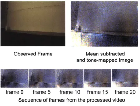
Observed Frame

Mean subtracted

and tone-mapped image

frame 0

frame 5

frame 10

frame 15

frame 20

Sequence of frames from the processed video

Figure 4-1: Top left: a representative frame of the seemingly static input video. Top right: a frame of the amplified residual video after subtracting the mean frame reveals blurry colored shadows and reflections. Bottom: a sequence of frames shows the motion of these features.

average out the noise, and tone-map the resulting signal to the full range of RGB values (often by a factor above 100), and add a middle-gray base level to account for the negative values. This procedure results in the sort of videos illustrated in Figure 4-1.

As a practical detail, a common but easily solved problem in video recording is that the light sources often flicker at the frequency of the alternating current. Despite using synced frame rates, we found that the signal of interest in amplified videos was

global sway.

We perform these operations in logarithmic space (with a small bias added to avoid zero) to equalize the magnitude of variations between dark and light regions of the scene.

This amplified video is of interest in itself, and sometimes reveals information which can be directly useful. For example, sharp-edged but previously invisible shadow silhouettes can become apparent. If the scene contains other objects than just a plain diffuse wall, amplified imperceptible specular reflections can also reveal a direct view to the hidden part of the scene. However, in most cases, the resulting video contains vague blurry shadows moving around in a manner that is suggestive of the motion taking place in the hidden scene, but hard to interpret visually.

4.2

Space-Time Plots for Classification

For these cases, we train a classifier to estimate the likely number of persons moving in the hidden scene, between zero, one or two persons. To this end, we further process the data to aid learning and inference.

Since the subjects are moving along the width of the observation plane, we average the video images over the vertical dimension of the signal to obtain a ID representation which captures the essential dimensions of the motion and improves the signal-to-noise ratio, while standardizing the data and eliminating most of the scene-specific nuisance factors in the full video. This collapses the video (W x H x T x 3) into an RGB space-time plot of dimensions W x T x 3.

Figure 4-2 shows examples of space-time plots for zero, one and two persons moving in the hidden scene. Figure 4-3 shows a typical relationship between the ground truth hidden scene motions and the observed space-time plot: while the tracks appear correlated, they are distorted and only partially observed.

Intuitively, these plots appear to show tracks of the moving people caused by the soft shadows, in some cases also revealing the color of the clothing worn by the subjects. Note that the space-time plots for the three classes look visually different.

0 Person 1 Person 2 Person f (D CO CL Time

-Figure 4-2: Examples of space-time plots for zero, one, and two people cases. As one of the spatial dimensions has been collapsed, the space and time dimensions can now be viewed as 2D images with time advancing towards right.

0 0 Cn C

11

W

Input

3 x

con, 5x5 con 5x5

batch norm batch norm conS 4x4 (no pad) mean-pool

leaky ReLU leaky ReLU batch nori over time FC 8 - 4 FC 4 - 3

mIax-pool 2x2 0 max-pool 2x2 leaky ReLLU dimension leaky ReLU softmax

8I 8

C = 3 8 4 64 8 42

C=3 W =64 cross-entropy

(RGB) loss

Figure 4-4: Convolutional neural network architecture used for classifying between 0,

1, and 2 persons.

Zero-person plots have little temporal variation, and simply show noise along the time dimension. One-person scenario looks relatively simple in terms of the visual texture of the plot, as compared to the plots for the two-people scenario. Since all the three classes show distinct visual differences and possess an image-like structure, this representation is suitable for learning to classify the scenarios using a convolutional neural network model.

4.3

Convolutional Neural Network Classifier

We formulate a simple CNN architecture for three-way classification between zero, one, and two people. The input to the network is a RGB space-time plot of dimension 64 x 256 x 3, that is, 64 pixels in spatial resolution and 256 time steps. Our data is standardized to zero mean and unit standard deviation prior to feeding it to the network. As our training dataset is small, we aim to keep the network as simple as possible to avoid overfitting.

Our neural network consists of 5 convolutional downsampling blocks, followed by mean-pooling over time, and two fully connected layers which output the prediction.

A diagram of the network architecture is presented in Figure 4-4. The convolutional

layers extract spatio-temporal features and gradually bring the size of the feature map down to the spatial resolution of 1 x 13, with 8 feature channels. This represents a summary of spatio-temporal features at 13 local time instances. The pooling opera-tion computes the temporal average, yielding a single 8-channel feature vector, which

is decoded by the final two layers into a predicted class. The idea behind the pooling is that our data is perfectly shift-invariant in time, and long-range correlations are not particularly meaningful - the pooling provides the network with means to aggregate local findings from different time instances into a joint statistic, which is used to form the final class estimate.

In the first four convolutional blocks, each convolution uses kernel size of 5 x 5, stride of 1, and uses zero-padding. The feature channel count in every intermediate layer is 8. The convolution in each block is followed by a leaky-ReLU non-linearity, and a 2 x 2 max-pooling layer to reduce the spatial and temporal dimensions. The leaky-ReLU layer uses a negative slope of 0.1

[19].

The fifth convolutional block is similar to the preceding ones, but has a convolution kernel size of 4 x 4 with no padding. This reduces the spatial dimension to 1 and temporal dimension to 13 time instants. These 13 feature vectors are collapsed using a mean-pooling operation over the time dimension, resulting in a 8-dimensional feature vector. This vector is the input to the linear layer followed by a leaky-ReLU, followed

by a final linear layer which outputs a vector with 3 values. We apply the softmax

function to the three-dimensional output to get the probabilities for the three classes. We use the standard cross-entropy loss.

We use the standard cross-entropy loss for the classification task. The neural net-work is trained using the RMSProp optimizer [211. We use learning rate of le' and decrease it by a factor of 10 every 20 epochs of training. The weights of the convolu-tion kernels are initialized using the He initializaconvolu-tion [22]. We train the network for 75 epochs as no meaningful change in performance appears beyond 40 epochs. The mod-els were implemented and trained using PyTorch [231. To improve the generalization of our model, we perform several data augmentations on our training data. These

Chapter 5

Results

In this chapter, we describe the real-world training and test data we collected, and evaluate the neural network model's performance on it. To gain insight into the data, we also perform an informal study on how difficult the task is for a human expert. Finally, we analyze the neural network's performance in controlled experiments with a synthetic data model.

5.1

Data Collection

In our experiments, we used 16-bit raw video captured using a PointGrey camera with a color sensor. All videos were captured at 15 frames per second, with shutter speed chosen based on the ambient light in the given environment. No extra lights were placed to illuminate the scene or to increase the signal reflected off the subjects. As our goal was to collect data from challenging scenarios, we made sure that the subjects were not casting direct sharp shadows on the wall. We collected data with people in 20 different scenes, consisting of interior spaces such as offices, conference rooms, classrooms, and public lounges. Each scene had a different room geometry and lighting conditions. In total, we collected 6 hours of video, split into roughly equal amount of time with one and two persons walking. The zero person case was collected separately in 10 different scenes which added up to half an hour of data.

two-person scenarios, the subjects would generally aim for independent movements, but occasionally moved in lockstep or otherwise mutually coordinated patterns.

5.2

Human Accuracy

To get a sense of the difficulty of the task, and of the characteristic features that the network might be able to take advantage of, one of the authors of the paper attempted the task of predicting zero, one, or two people based on the same space-time plots input to the CNN. The author achieved an overall accuracy of 84%, which breaks down to 100% on the zero person cases and 73% for distinguishing between one and two person cases on a sample set of 1000 images.

One of the key features considered while evaluating the space-time plot was the apparent complexity of their texture. The zero person case showed an almost con-stant value along the time dimension of the space-time plot. One person cases were characterized by a single track while space-time plots for the two person cases had the most complicated textures. Most of the failure cases were two person cases mis-classified as one, which in most cases were attributed to scenarios where both people were moving with similar velocities.

We also observed a common effect useful for discrimination in two-person space-time plots, where a sharp vertical line would somespace-times appear on the plot when the persons crossed one another. This is apparent in Figures 4-2 and 4-3; see in particular the middle part of the two-person track in the latter. This abrupt change in intensity of the wall appears when one person obscures the other from the wall, and for a brief instant the scene is effectively only shadowed by one person.

Accuracy

Test on 0 person case 0.98

Test on 1 person case 0.722

Test on 2 person case 0.878

Average Test Accuracy 0.86

Table 5.1: Average model performance on the 3 classes

Accuracies across scenes (sorted in descending order)

-* - Test Accuracy for 0 people I

-@- Test Accuracy for 1 person

-0 - Test Accuracy for 2 people

-4- Overall Test Accuracy I

- Random Guess I ll I -'-~ i~I '* ii ii I~I i~ I I ~I I I I ii I ID I

4'

Scene Number

Figure 5-1: Accuracy of the model across scenes.

rooms, the network is always tested on novel conditions (i.e. a new room). For the zero person testing, we simply randomly hold out one of the zero-person scenes in each of these folds.

Table 5.1 shows the average test accuracy of the model on each of the 3 classes across all scenes. Since the zero person case is simple, the model achieves an accuracy of 98% on unseen test data. The model performs relatively better on the two-person case with 87.8% correct predictions, as compared to the one-person case where it achieves an accuracy of 72.2%.

Figure 5-1 breaks down the accuracy of the model for each individual scene. The scenes are sorted in descending order by average test accuracy. For most of the scenes,

1.0

-0.8

-

0.6-

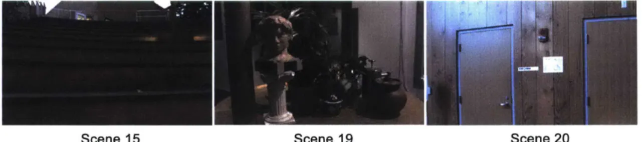
0.2-Scene 15 Scene 19 Scene20

Figure 5-2: Observation image of the setup for the stress tests.

the model performs relatively equally on all classes. In some of the scenes, it shows a biased behavior of performing relatively worse on one of the classes, which in most cases is the 1 person case.

5.4

Stress Test Scenes

To explore the limits of the model, we captured three scenes which violate our assumptions in one way or another. These are marked as Scenes 15, 19, and 20 in Figure 5-1. Figure 5-2 shows an example frame from each one of these sets.

In Scene 15, we tested our method in an outdoor setting in the evening. This is a difficult case, as it is the only outdoor scenario in the dataset. Moreover, the light conditions were dark, and consequently the signal to noise ratio is unusually low. Nevertheless, the network is not completely unsuccessful with this scene.

Emitter plane

person #2

Observation plane

Figure 5-3: Two-dimensional flatland setup for synthetic data generation. The two blockers representing persons move back and forth along random directions. A ID image is rendered at the observation plane, taking into account the mutual visibility between the blockers and the back wall acting as an illuminant.

5.5

Analysis with Synthetic Data

To run controlled experiments with the classifier, we formulated a synthetic data generation pipeline that simulates our imaging setup in a simplified 2D "flatland" sce-nario. In particular, we are interested in the classification performance as a function of the relative motion patterns for two people.

The flatland setup consists of two parallel walls - a receiver wall that is observed, and an emitter plane that emulates the lighting environment, as shown in Figure 5-3. Between these, one or two flat occluders move in distorted sinusoidal patterns. The light transport is simulated according to an approximate two-dimensional version of the rendering equation. The lighting environment, diffuse albedo variation on receiver, occluder colors, motion patterns, ambient lighting, noise, and other aspects of the simulation are randomized.

Figure 5-4 shows a selection of one and two-person space-time plots generated in this manner. While not fully identical to the real data, the plots show similar qualitative effects - for example, the streaks resulting from cross-overs discussed in Section 5.2 can also be seen in these plots. Our classifier trained with all of the real data achieves an overall accuracy of 67.5% in one-vs-two classification for the synthetic test dataset of 14,000 samples, demonstrating reasonable generalization to data obtained by significantly different means.

(a) (b)

Figure 5-4: (a) Samples of synthetic space-time plots for one person scenario. (b) Samples of synthetic space-time plots for two people, in the same scenario as (a).

This suggests that the synthetic data has a good level of realism, and that it can be meaningfully used to run controlled experiments that would be hard to arrange with real data. In order to study the impact of relative motion, we generated a dataset of two persons moving in various parameterized sinusoidal patterns under 80 different scenes, and studied the average classification performance (i.e. whether the segments were correctly classified as two-person cases) as the parameters were varied. Specifically, we set person 1 to move in a standard sinusoidal pattern, and vary the relative frequency, amplitude and phase of person 2's movements. Figure 5-5 shows the results of this analysis along different axes of variation.

Figure 5-5a shows the overall effect of varying the relative amplitude and frequency of person 2's movement. The poorest classification performance is attained when

Average accuracy across all phase values

I

Relative Amplitude

(a)

Accuracy for same frequency of the subjects -2.0 0 -0.3 -0.6 0 -0.4 . -0.2 -0.0 Relative Amplitude (b)

Average accuracy across variation in the relative frequency.

1.0- 0.9-0.8. i Relative Frequency (c)

Average accuracy across variation in the relative amplitude.

1 n . 0.9-0.8 U $ 0.7 U U 0.6 0.5 ---V.125 Relative Amplitude (d)

Figure 5-5: Classification performance for synthetic two-person video segments as a function of different relative motion parameters.

0.5 >1 0U ar LU 1 U U 6 5 ---1.0 -0.8 -0.6 '0.2 -0.0

0.

0

Figure 5-5b analyzes the special case when both persons are moving at the same frequency, but their relative phase and amplitude are varied. As expected, the clas-sification performance is low when the persons move in lockstep, i.e. when the phase difference is small. The lowest performance is reached when the motions are also of equal amplitude, namely identical. In contrast, opposite-phase and equal magnitude motion appears to be resolved best - presumably because in this case the signals from the persons are maximally different while being least likely to drown one another out. The generally successful classification for equal-frequency cases shows that perfor-mance is not affected when the two-person data is a one-dimensional manifold, ruling out that the network would be simply performing a dimensionality analysis of the data. This suggests that the network is taking advantage of visual cues such as those discussed in Section 5.2.

We also experimented with using synthetic data to augment the training. This yielded a positive but insignificant additional benefit over the purely real-data train-ing.

Chapter 6

Conclusion

We show that it is possible to infer the number of people in a non-line-of-sight

scenario by a simple passive observation of a blank wall. The changes in indirect illumination, due to soft shadows and secondary reflections, show signals on the ob-servation plane (on a wall), presenting a view of the dynamic activity in the hidden scene. These signals are sufficient to be analyzed by a simple neural network work-ing with a 2D space-time projection of the input video for the task of countwork-ing the number of people. In addition to results on real scenes, we analyzed the performance of the approach with synthetic data specifically on the two person case. Our analysis shows that, as expected, correlated movement of the 2 persons results in the hardest scenario for our method.

Bibliography

[1] Felix Naser, Igor Gilitschenski, Guy Rosman, Alexander Amini, Fredo Durand,

Antonio Torralba, Gregory W Wornell, William T Freeman, Sertac Karaman, and Daniela Rus. Shadowcam: Real-time detection of moving obstacles behind

a corner for autonomous vehicles. In 2018 21st International Conference on

Intelligent Transportation Systems (ITSC), pages 560-567. IEEE, 2018.

[2]

in-dustrial environments: Seeing around corners. In 2012 IEEE/RSJ International Conference on Intelligent Robots and Systems, pages 4231-4232. IEEE, 2012.

[3] Fadel Adib, Chen-Yu Hsu, Hongzi Mao, Dina Katabi, and Fr6do Durand.

Cap-turing the human figure through a wall. A CM Trans. Graph., 34(6):219:1-219:13, October 2015.

[41 Fadel Adib and Dina Katabi. See through walls with WiFi!, volume 43. ACM,

2013.

[5] Saandeep Depatla, Arjun Muralidharan, and Yasamin Mostofi. Occupancy

esti-mation using only wifi power measurements. IEEE Journal on Selected Areas in Communications, 33(7):1381-1393, 2015.

[6] Achuta Kadambi, Hang Zhao, Boxin Shi, and Ramesh Raskar. Occluded imaging

with time-of-flight sensors. ACM Transactions on Graphics (ToG), 35(2):15,

2016.

[7] Felix Heide, Matthew O'Toole, Kai Zang, David Lindell, Steven Diamond, and

Gordon Wetzstein. Non-line-of-sight imaging with partial occluders and surface normals. arXiv preprint arXiv:1711.07134, 2017.

[8] Katherine L Bouman, Vickie Ye, Adam B Yedidia, Fr6do Durand, Gregory W

Wornell, Antonio Torralba, and William T Freeman. Turning corners into cam-eras: Principles and methods. In Proceedings of the IEEE International

Confer-ence on Computer Vision, pages 2270-2278, 2017.

[9] Manel Baradad, Vickie Ye, Adam B Yedidia, Fr6do Durand, William T Freeman,

Gregory W Wornell, and Antonio Torralba. Inferring light fields from shadows. In Proceedings of the IEEE Conference on Computer Vision and Pattern Recog-nition, pages 6267-6275, 2018.

[10] Charles Saunders, John Murray-Bruce, and Vivek K Goyal. Computational

periscopy with an ordinary digital camera. Nature, 565(7740):472, 2019.

[11] Fadel Adib, Zach Kabelac, Dina Katabi, and Robert C Miller. 3d tracking via

body radio reflections. In 11th

{

Design and Implementation ({NSDI} 14), pages 317-329, 2014.

[12] Andreas Velten, Thomas Willwacher, Otkrist Gupta, Ashok Veeraraghavan, Moungi G Bawendi, and Ramesh Raskar. Recovering three-dimensional shape around a corner using ultrafast time-of-flight imaging. Nature communications,

3:745, 2012.

[13]

objects outside the line of sight using speckle imaging. In Proceedings of the

IEEE Conference on Computer Vision and Pattern Recognition, pages

6258-6266, 2018.

[14] Matthew O'Toole, David B Lindell, and Gordon Wetzstein. Confocal non-line-of-sight imaging based on the light-cone transform. Nature, 555(7696):338, 2018.

[15] Hao-Yu Wu, Michael Rubinstein, Eugene Shih, John Guttag, Fr6do Durand, and

William Freeman. Eulerian video magnification for revealing subtle changes in the world. 2012.

1161

[17]

[18] Ravi Ramamoorthi and Pat Hanrahan. A signal-processing framework for inverse

rendering. In Proceedings of the 28th Annual Conference on Computer Graphics and Interactive Techniques, SIGGRAPH '01, pages 117-128, New York, NY,

[22] Kaiming He, Xiangyu Zhang, Shaoqing Ren, and Jian Sun. Delving deep into rec-tifiers: Surpassing human-level performance on imagenet classification. In

Pro-ceedings of the IEEE international conference on computer vision, pages

1026-1034, 2015.

[23] Adam Paszke, Sam Gross, Soumith Chintala, Gregory Chanan, Edward Yang,

Zachary DeVito, Zeming Lin, Alban Desmaison, Luca Antiga, and Adam Lerer. Automatic differentiation in pytorch. 2017.