Centrality metrics in dynamic networks: a comparison study

HAL Id: hal-01925647

https://hal.archives-ouvertes.fr/hal-01925647

Submitted on 16 Nov 2018

HAL is a multi-disciplinary open access

archive for the deposit and dissemination of

sci-entific research documents, whether they are

pub-lished or not. The documents may come from

teaching and research institutions in France or

abroad, or from public or private research centers.

L’archive ouverte pluridisciplinaire HAL, est

destinée au dépôt et à la diffusion de documents

scientifiques de niveau recherche, publiés ou non,

émanant des établissements d’enseignement et de

recherche français ou étrangers, des laboratoires

publics ou privés.

Centrality metrics in dynamic networks: a comparison

study

Marwan Ghanem, Clémence Magnien, Fabien Tarissan

To cite this version:

Marwan Ghanem, Clémence Magnien, Fabien Tarissan. Centrality metrics in dynamic networks: a

comparison study. IEEE Transactions on Network Science and Engineering, IEEE, 2018, pp.1 - 1.

�10.1109/TNSE.2018.2880344�. �hal-01925647�

Centrality metrics in dynamic networks: a

comparison study

Marwan Ghanem

, Cl ´emence Magnien

and Fabien Tarissan

∗

_{Sorbonne Universit ´e, CNRS, Laboratoire d’Informatique de Paris 6, LIP6, F-75005 Paris, France}

_{Universit ´e Paris-Saclay, CNRS, ENS Paris-Saclay, ISP UMR 7220, France}

Abstract—For a long time, researchers have worked on defining different metrics able to characterize the importance of nodes in static networks. Recently, researchers have introduced extensions that consider the dynamics of networks. These extensions study the time-evolution of the importance of nodes, which is an important question that has yet received little attention in the context of temporal networks. They follow different approaches for evaluating a node’s importance at a given time and the value of each approach remains difficult to assess. In order to study this question more in depth, we compare in this paper a method we recently introduced to three other existing methods. We use several datasets of different nature, and show and explain how these methods capture different notions of importance.We also show that in some cases it might be meaningless to try to identify nodes that are globally important. Finally, we highlight the role of inactive nodes, that still can be important as a relay for future communications.

Index Terms—centrality, network dynamics, temporal paths, node importance

F

1

INTRODUCTION

Scientists studying complex networks have been inter-ested for a long time in the question of evaluating the importance of a node. This has led to the introduction of several measures of importance, such as for instance degree, closeness or betweenness centrality, Eigenvector centrality or Katz centrality, or PageRank.

Many centrality measures are based on the study of paths in the network. In this approach, a node will be important if the paths from it to other nodes are short in average, or if it lies on the shortest paths between sev-eral pairs of nodes. One motivation is that links can act as a dissemination medium for an information spreading on the network. For instance, individuals can exchange information when they communicate, or a message can be forwarded from computer to computer until it reaches its destination.

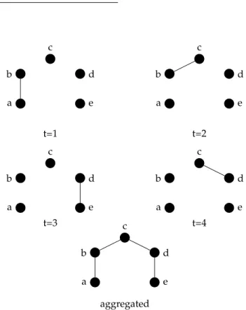
Researchers started to focus on static networks first as they represent many real-world situations, such as protein interaction networks or food chain networks, among others. However, other cases of interest include temporal aspects, such as email exchanges between individuals occurring at different points in time. Such networks were first analyzed and modeled statically for the sake of simplicity but this representation induces a strong loss of information. Indeed, in the case of path based centralities, the order of links is completely lost and paths that do not respect time exist in the time-aggregated version of a dataset. To observe this, consider the toy example of Figure 1. This small network composed of five nodes evolves during four distinct time steps. By discarding the temporal aspect and aggregating all links into a single network, we can observe that a path from a to e exists although no transmission between a and e is possible in the temporal network.

This has led to a stream of works aiming at under-standing and modeling these dynamics. In particular, in the case of centrality, some works have been concerned with

c b a d e t=1 c d e b a t=2 c d e b a t=4 c b a d e t=3 _c d e b a aggregated

Fig. 1: A small example of a dynamic network. The links existing at time t = 1 are shown on the top left corner, the ones existing at t = 2 in the top right corner, and so on, and

the aggregated network is shown last.

efficiently updating the centrality values of the nodes when a change occurs in the network. In many cases however, the time scale at which the network evolves is the same as the one at which a dissemination phenomena may occur on the network. This is the case for instance when a disease propagates among individuals when they are in contact, or when information is disseminated by emails.

One very important point concerning centrality in dy-namic networks is that while paths change during the network time span so does the importance of nodes. Con-sider again the toy example of Figure 1. One can see that, intuitively, the importance of node b is stronger at time t = 1 than at time t = 3. Indeed, at time t = 1 it forms a bridge between node a and nodes c and d, thanks to the link that exist at t = 2. This is in contrast with its situation at time t = 3 where it cannot be used as a relay anymore.

Several works have introduced extensions of centrality notions for the case of dynamic networks. In this paper, we study four such extensions proposed in the literature. We compare these extensions on several datasets from which we conclude that:

1) perception of the importance of a node strongly

depends on the centrality metric used, raising the question of the desired characteristics of a dynamic centrality metric;

2) the dynamic of the network might be such that it

is meaningless to identify nodes which are more important than others;

3) metrics react differently to the different natures of

datasets;

4) a node can be inactive (i.e. not have any links) at a

given time, yet be highly important as it may serve as a relay for future communications.

This work is organized as follows. First we present in Section 2 the existing work related to the notion of centrality in static and dynamic networks. We present in details the four methods we study here in Section 3, before providing our methodology of comparison in Section 4. We present the datasets we use for the comparison in Section 5 and the results we obtained in Section 6 before concluding the paper in Section 7.

2

RELATED WORK

Many papers have studied the importance of nodes in static networks, i.e. networks that don’t evolve with time. Among the metrics that have been introduced, one may cite the degree centrality, closeness centrality [1], betweenness cen-trality [2] and the Katz [3] and eigenvector centralities [4], [5]. Closeness and betweenness centralities are based on shortest paths, while the Katz centrality takes into account paths of all lengths between two nodes.

Some papers which have studied dynamic networks have been concerned with efficiently computing the static centrality at all times. For instance, Kas et al. [6] propose an algorithm that, given distances between all pairs of nodes and given a network change (edge appearance of disappearance), computes the new centrality measure by updating the distance values rather than computing them all from scratch again. This is relevant, e.g. in contexts where the network evolves at a much slower scale than the one on which a dissemination takes place.

One of the first methods attempting to account for the evolution of temporal networks is the snapshot method. In this approach, the network timeline is divided into several periods, and all nodes and links that exist in this period are

aggregated into a snapshot network; each snapshot is then analyzed separately using a static metric. Uddin et al. [7] propose a framework that, given a static centrality measure, computes it for each period. This method proves to be better than a static analysis. Another approach [8] studies the dy-namicity of nodes. The authors introduce two metrics which quantify the change in importance and presence of a node in a dynamic network. This approach is subtly but really different from a study of the time evolution of a node’s importance. Braha et al. [9] also use the snapshot approach. However, in addition to detecting important nodes, they detect cycles as well. Similarly Tang et al. [10] consider the same aggregation while keeping the edge order in each snapshot. They are thus more accurate as they only take into account paths that are temporally possible. All in all, the inconvenience of these aggregation variants remain: each centrality value represents the centrality for a period rather than an exact instant, leading to information loss.

In many contexts, the dissemination phenomenon in the network happens on the same time scale as the network evolution. It then becomes necessary to consider temporal paths [11], [12], i.e. link sequences that are time-respecting. For instance, in the dynamic network of Figure 1, there is a temporal path from node a to node c going through the link (a, b) at t = 1 and the link (b, c) at time t = 2.

Several definitions of temporal paths have been studied in the literature. Some of them can be computed more easily than others. Whitbeck et al. [13] propose an efficient algorithm to approximate the existence of paths in the most difficult case and show that the notion of reachability (i.e. which nodes can be reached from which nodes, and at which times in the network’s time span) provides enlightening insight on the network’s dynamics.

Notions of centrality taking into account temporal paths have also been introduced. Nicosia et al. [14] introduce the notions of temporal closeness and betweenness centralities. However, their definition of a shortest path considers only paths whose starting point is at the beginning of a dataset’s time span.

Scholtes et al. [15], [16] introduced another approach to take into account all temporal paths. They introduced a higher order aggregation where each node represents a possible temporal path. In addition, they introduce several temporal centrality definitions, including a temporal cen-trality that represents a node’s importance at each instant, which is, however, too costly to compute except for small examples.

Another approach consists in depicting the dynamic network as a static network [17], [18], by creating one copy of each node for every instant, and linking two consecutive copies of the same node by a (directed) link. This repre-sentation allows to consider temporal paths while using classical centrality metrics. However, using this represen-tation is compurepresen-tationally expensive and remains unfeasible particularly for highly active datasets.

Various other propositions acknowledge that the dis-tances between nodes, and therefore, nodes’ importance, vary with time [9], [12], [19], [20], [21], [22]. However, in practice, they still represent the varying importance of a node by a single value that is supposed to represent its overall importance throughout the network global time

span.

Several papers introduce and study variants of the Katz or eigenvector centralities [23], [24]. Among those, Lerman et al. [25] acknowledge the fact that a node’s importance may evolve with time, but no systematic study is conducted. Moreover, their variant relies on parameters defining what is to be considered as relevant path lengths and path dura-tion, which complicates the analysis. Fenu et al. [26] explore the different methods for representing a dynamic network as a block matrix where each column/row corresponds to a pair composed of a node and a time instant. They propose a method to construct such a block matrix that allows to compute dynamic centrality metrics in an efficient way. Taylor et al. [27] introduce such a block matrix (that they call supra-centrality matrix) and study the corresponding eigenvector centrality.

Finally, Costa et al. [28] notice that not all time instants are equivalent in a dynamic network, and introduce the notion of time centrality. This measures how fast a dissemination process can reach a significant portion of the nodes at a given time t. However, this notion is global and does not describe the importance of individual nodes in the dissemination process.

All in all, several papers acknowledge the fact that the temporal evolution of networks impact the value of cen-trality measures and propose variations of standard metrics to account for the dynamics. However, and to the best of our knowledge, very few analysis of the difference between these methods have been performed. This paper intends precisely to contribute in this direction, by comparing four different methods that evaluate the importance of a node based on different criteria.

3

TEMPORAL CENTRALITY DEFINITIONS

In this section we present the four methods that we will compare in the rest of the paper.

3.1 Temporal Closeness

The first method was previously presented in [29]. A

dy-namic network G = (V, E) consists of a set V of nodes1_and

a set E of timed links of the form (u, v, t) where u, v ∈ V and t is a timestamp. Throughout the paper we consider networks as undirected, i.e. a link (u, v, t) is equivalent to a link (v, u, t).

A temporal path in a dynamic network consists of:

• a starting time ts, and

• a sequence of links

(v0, v1, t0), (v1, v2, t1), . . . , (vk, vk+1, tk)

such that:

1) for all i, i = 0..k − 1, ti < ti+1,

2) t0> ts.

We say that such a path is a path from v0to vk+1starting

at time ts. Its duration is equal to tk− ts. We say that a path

from u to v starting at time tsis a shortest path if it has the

least duration among all paths from u to v starting at time

1. We assume that the set of nodes does not evolve with time.

ts. We define the (temporal) distance from u to v at time ts

to be the duration of a shortest path from u to v starting at

ts, and we denote it by dts(u, v). If there is no path from u

to v starting at time ts, we consider that dts(u, v) = ∞.

Note that a path starting at time tsmight imply waiting

times at all nodes, including the first one, in the same way that a person starting a train trip with connections at a given time must wait for the train in the first station, and then at each connecting station.

If we consider the dynamic network of Figure 1, there is a temporal path from b to d starting at time t = 1. The path consists of the links (b, c, 2) and (c, d, 4) and its duration is 3. The temporal distance from b to d at time 1 is therefore

d1(b, d) = 3 (there is no path that starts at time 1 and arrives

earlier).

We recall that the closeness of a node u in a non-evolving network is defined as [1]:

X

v6=u

1

d(u, v),

where d(u, v) is the classical graph distance.

Similarly, we define the temporal closeness of a node u at time t as: Ct(u) = X v6=u 1 dt(u, v) .

Note that the strict definition of Ct(u) requires to

com-pute the value for each time instant t. For obvious compu-tational reasons (one of the dataset we use in this study is a record spanning 3 years), we only compute the temporal closeness for each node every I seconds. The value of I is equal to the median of inter-link duration (i.e. the time

separating two consecutive links)2. We argue that this fixed

frequency is precise enough to get an accurate information when compared to computing the temporal closeness at every second.

3.2 Closeness Snapshot

The second method was proposed by Uddin et al. [7]. In

this framework, a temporal network Gtis represented as a

sequence of static networks (snapshots), each to be analyzed separately. Each static network is the aggregation of all the links in a given period and all the snapshots represent peri-ods of equal duration. Given a static centrality measure for each snapshot (such as the classical definition of closeness), the framework computes this centrality for all nodes.

Note that for the comparison with the temporal closeness presented above, we consider the closeness value of a node is the same every I seconds in a given snapshot. We denote this method by SnapshotCl.

3.3 Temporal Eigenvector

The third method was presented by Taylor et al. [27]. They represent temporal networks as a supra-centrality matrix of size N T × N T , where N is the number of nodes and T is the number of considered time periods. This matrix con-tains one static centrality matrix (for example an ordinary

2. The program we used to compute the metrics is publicly avail-able [30].

A > B = C = D = E > F | {z } centrality Relation =⇒ 5 1 1 1 1 0 | {z } ranks

Fig. 2: An example of inverse competition ranking.

adjacency matrix for the eigenvector centrality) for each time period. These matrices are placed on the diagonal of the supra-centrality matrix. Other links are added to couple these centrality matrices with each other. The dominant vec-tor of this supra-centrality matrix would give the centrality for each node i at each time t.

In the following, we call this method Temporal Eigenvec-tor. We will consider that each period has a duration of I seconds.

3.4 Coverage Centrality

The fourth method was presented by Takaguchi et al. [17]. It represents a temporal network as a static network where each temporal node consists of a pair composed of a node (of the original network) and a time instant. Consecutive

pairs of the form (u, t1) and (u, t2) sharing a same node

u are linked, and temporal links between nodes u and v at time t are represented by two links: one from (u, t) to (v, t + 1), and the symmetric link. This allows to represent temporal networks statically while keeping the temporal order between the links. Building on this representation, the authors introduce two centrality notions. First, temporal coverage centrality represents the importance of a temporal node (u, t) by the fraction of pairs of nodes for which a shortest path passes through the node (u, t). A variant, called temporal boundary coverage centrality, has been defined. In this study, we only consider the temporal coverage centrality. Preliminary results, however, revealed that both centralities behave quite similarly on our datasets.

4

COMPARISON

The four approaches described in the previous section pro-pose very different ways to quantify the importance of a node in a dynamic network, thus making it difficult to directly compare the raw values. In the rest of the paper we will therefore rely on the following additional steps to compare the methods.

4.1 Ranking

Evaluating the importance of a node with respect to the others by considering only its centrality value is difficult. Therefore, in order to obtain an intuition on the node’s rela-tive importance, we rank them at each time step with respect to their centrality values. We chose the inverse competition ranking method. In this ranking, the ranking 0 is attributed to the least central nodes, and the ranking of every node is equal to the number of less central nodes. Consider the example in Figure 2, which consists of 6 nodes with their centrality relationship in addition to their attributed ranks. The ranking 0 is attributed to F which is the least central node, while nodes B, C, D and E share the same ranking 1 as they are all equally important. Finally, A is ranked 5.

We will use this ranking approach to compare properly the results of the different methods.

First, given two rankings obtained by two different methods for the same network at the same time step, we can compute their correlation as defined by the Kendall-Tau coefficient. This coefficient has a value in [−1, 1] that represents the level of concordance between the two ranking lists. 1 stands for a perfect correlation while −1 stands for a perfect negative correlation. More precisely, we compute the difference between the number of concordant and dis-cordant pair of nodes between the two lists, a condis-cordant pair of nodes being a pair for which the two nodes have the same relationship in both ranking lists. So a pair (u, v) is said to be concordant if either u is ranked higher than v in both ranking lists, or u is lower than v in both ranking lists, or u has the same ranking as v in both ranking lists. We then normalize this value by the number of pairs in order to obtain a final value between −1 and 1. We compute this correlation at each instant to study its evolution over time.

Second, while it is interesting to know how much the rankings obtained by different methods differ globally, this does not provide any intuition on the difference of impor-tance attributed to any given node in particular. In order to deepen our understanding, we will therefore also compute for every node the difference between the two ranks. A high difference thus indicates that the two rankings have a strong divergence regarding the importance of the con-sidered node, while a value close to 0 indicates that they both agree on its relative importance in the network. We will study the distribution of the rank difference over all pairs consisting of a node and a time instant.

4.2 Global importance

In order to provide a more comprehensive and global perspective of the importance of all nodes at each time instant, we will study the number of times any given node is attributed a high (or low rank). The idea is that a node that is consistently assigned a high rank is evaluated as globally important. More formally, we define two regions, which we call top and bottom, representing respectively the top 25% ranks and the bottom 25% ranks. Considering a network of n nodes, a node with a ranking higher than bn ∗ 0.75c is therefore considered to be in the top region while a node with a ranking lower than bn∗0.25c is considered to be in the bottom region. This allows to detect immediately which are

the nodes of high or low global importance in a network3.

Finally, we compute for each node the total duration

spent in each region and we denote it by Durtop (resp.

Durbot). To compute these durations, we consider that a

node is present in the top or bottom region from the instant where we compute the centrality to the next computing

instant: given a node u ∈ V , if R(u) = (ri)i=1...k is the

sequence of ranks (computed at instants i = 1..k) for u, we

define Durtop(u) and Durbot(u) as :

Durtop(u) = I · |{i ≤ k − 1, ri≥ bn ∗ 0.75c}| ,

Durbot(u) = I · |{i ≤ k − 1, ri≤ bn ∗ 0.25c}| .

3. it is worth noticing that, because the inverse competition ranking may assign the same ranking to several nodes, these regions may contain more than or less than25%of the nodes.

5

DATA

SETS

In order to compare and understand the differences between the different methods, we study several datasets coming from different contexts and presenting different character-istics:

• Enron [31]: this dataset contains the 47 088 emails

that 151 Enron employees exchanged during approx-imately three years. It records information on the senders, receivers, and the moment they were sent.

• Radoslaw [32]: this dataset contains 82 876 emails

exchanged by 168 employees of a mid-sized com-pany during a period of nine months in 2010. It records information on the senders, receivers, and the moment they were sent.

• Rollernet [33]: this dataset was collected during a

rollerblading tour in Paris in August 2006. The tour is a weekly event and gathers approximately 2 500 participants. Among these, 62 were equipped with wireless sensors recording when they were at a communication distance from one another. The total dataset duration is approximately 2 hours and 45 minutes (note that there is a break of approximately 30 minutes during the tour).

• Twitter (HashTags): A 22 day long twitter dataset

generated by twitter accounts known to be associated with terrorist groups. Each node represents a hash-tag, while each link represents a tweet that contained the two hashtags. Thus, a tweet with several hashtags generates several links. The dataset contains 3 048 hashtags and 100 429 links.

• Twitter (Retweets): From the same twitter dataset,

we extracted a subset of 27 919 re-tweets generated by the 10 484 twitter accounts. Each link (u, v, t) represents a user v re-tweeting a tweet of user u at time t.

• Facebook [34]: this dataset is a 1 year long record of

the activity of Facebook users between 31st of De-cember 2015 and 31st of DeDe-cember 2016. The dataset contains 8 977 Facebook users and their 66 153 posts to each other’s wall on Facebook. The nodes of the network are users, and each link represents a user writing on another user’s wall.

In all cases, we consider that links are undirected. In order to apply the snapshotCl method on these networks, we need to choose a snapshot duration. Choosing the ap-propriate value is in general a difficult question as this impacts the obtained results [35], [36], [37]. We chose the value that gave a good compromise between a low loss of temporal information (i.e., a low aggregation and hence a small snapshot duration) and a sufficiently high number of active nodes, so each snapshot contains relevant informa-tion. We show that the choice of the snapshot duration has little impact on our observations in Section 7 and in the supplementary material.

The main global characteristics of these datasets, includ-ing the chosen snapshot duration, are presented in Table 1. In the rest of the paper, for the sake of brevity and because the observations on some datasets are similar, we will only present the results on three of the datasets: Enron, RollerNet, and Twitter (HashTags). Before comparing the methods, it is

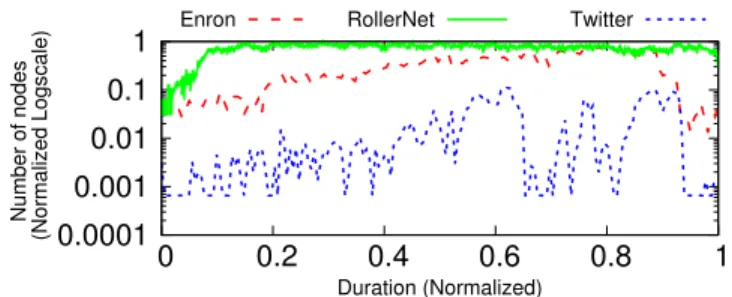
0.0001 0.001 0.01 0.1 1 0 0.2 0.4 0.6 0.8 1 Number of nodes (Normalized Logscale) Duration (Normalized) Enron RollerNet Twitter

Fig. 3: Time-evolution of the proportion of active nodes.

enlightening to make some global observation related to the dynamic of the three networks.

For each dataset, we computed the proportion of active nodes in a snapshot (i.e. the fraction of nodes having at least one link during the corresponding period). Figure 3 shows the time evolution of this value for the three datasets. In the Enron case, the proportion increases slowly to a maximum of 80% before dropping drastically at the very end. In the RollerNet case, the proportion of active nodes increases rapidly and remains very close to 1 until the end. Finally, in the Twitter dataset, we can see that the activity is extremely low compared to the two other datasets, with only very few nodes active in each snapshot. Thus, those three cases present very different characteristics in terms of activity. We conjecture that this has a strong impact on the way node’s importance is perceived by the different methods. We will investigate this question in the next section.

6

RESULTS

In this section, we compare how the different methods presented in Section 3 quantify the importance of nodes in a dynamic network. We start by analyzing the global difference between the methods (Section 6.1) before eval-uating how this difference impacts the relative importance of individual nodes (Section 6.2). Finally, we compare which nodes are identified by the methods as globally important over the whole period of time (Section 6.3).

Note that temporal closeness, snapshotCl and temporal eigenvector have been computed for all datasets but the coverage centrality was too computationally expensive to be used on another dataset than Enron.

6.1 Global observations

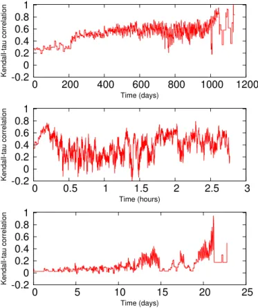
We start by comparing temporal closeness with snapshotCl. Figure 4 presents the evolution of the Kendall-tau correla-tion between the rankings provided by the two methods for the three datasets. For Enron (Figure 4, top), the cor-relation is low at first and then increases over time. At the beginning, a large number of nodes are inactive and snapshotCl attributes the lowest rank (0) to all of them. However, temporal paths involving links that appear later in the dataset exist from most of these nodes. Therefore, a non-zero value (and hence a non-zero rank) is attributed by the temporal closeness to these nodes. Naturally, as the network evolves, more nodes become active and are

Datasets |V | |E| Duration I (Seconds) Snapshot duration

Enron 151 47 088 3 years 960 1 week

Radoslaw 168 82 876 9 months 53 1 week

RollerNet 62 403 834 3 hours 4 1 minute

Twitter

(HashTags) 3 048 100 429 22 days 16 3 hours Twitter

(Retweets) 10 484 27 919 20 days 18 1 hours

Facebook 8 977 66 153 1 year 278 1 week

TABLE 1: number of nodes |V |, number of links |E|, dataset duration, median of inter-link duration (I) and snapshot duration for each dataset.

-0.2 0 0.2 0.4 0.6 0.8 1 0 200 400 600 800 1000 1200 Kendall-tau correlation Time (days) -0.2 0 0.2 0.4 0.6 0.8 1 0 0.5 1 1.5 2 2.5 3 Kendall-tau correlation Time (hours) -0.2 0 0.2 0.4 0.6 0.8 1 0 5 10 15 20 25 Kendall-tau correlation Time (days)

Fig. 4: Time-evolution of the Kendall-Tau correlation between temporal closeness and snapshotCl. Top: Enron;

Middle: Rollernet; Bottom: Twitter.

then taken into account by snapshotCl, which increases the

correlation between the two methods4_.

The effect of inactive nodes spotted above is not re-stricted to the beginning of the evolution. One might notice for instance that the correlation drops suddenly at certain instants, even close to the end of the trace. Manual investi-gation revealed that this corresponds to moments where a significant number of nodes are temporarily inactive. This generates a strong difference between temporal closeness and snapshotCl for the same reason than above. We later on refer to such instants as temporary inactive moments.

Finally, at the end of the evolution, the correlation

4. note that nodes that were active in the past but do not have any future links are attributed a rank of 0 by both methods.

reaches very high values; this is due to a large number of nodes inactive and ranked 0 by both methods, which makes it hard to have a high difference in the global rankings.

In contrast with the Enron dataset, if we now consider the RollerNet dataset (Figure 4, middle), we can see that the Kendall-tau correlation 1) fluctuates highly, 2) is globally lower, and 3) can even be negative at some instants. This observation is clearly related to the high activity of the nodes (see Fig. 3). This activity leads the networks of each snapshot to be much denser than in Enron. As we highlighted in Sec-tion 2, this makes snapshotCl more likely to consider paths that are temporally impossible, thus leading to divergence with temporal closeness.

Finally, we focus on the Twitter dataset (Figure 4, bot-tom). Since the dataset is the least active and contains mostly temporary inactive moments, the correlation is pretty low. At the beginning most nodes are inactive; the number of active nodes becomes significant only after the 14-th day. This is why the correlation starts to increase at that time. Finally, one can identify several periods of high correlation which are strongly related to periods with a high number of active nodes (see Figure 3).

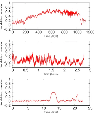
We now turn to the comparison with temporal eigen-vector. Figure 5 shows the evolution of the correlation between temporal closeness and temporal eigenvector for the three datasets. For Enron (Figure 5, top), the correlation fluctuates and globally increases with time, before dropping as the total activity drops (around the 1000-th day). This shows that both methods are only correlated when there is a relatively high activity. Interestingly, though we would expect the correlation to increase at the very end, as previ-ously seen with snapshotCl, it actually decreases. If we now consider the Rollernet dataset (Figure 5, middle), we can see how the correlation fluctuates as seen previously. We notice that the correlation is quite low. This further indicates that both methods do not have the same notion of importance. Finally, for the Twitter dataset (Figure 5, bottom), we can see how the correlation is quite low and constant, with two peaks that correspond to a clear increase of the activity. This further shows that both methods produce different results when the activity is low. This is probably due to the observation made by Fenu et al. [26] that Temporal Eigenvector considers paths that do not respect time and can therefore go backwards in time. This explains why nodes that are permanently inactive at the end of the dataset can have a non-zero rank.

-0.2 0 0.2 0.4 0.6 0.8 1 0 200 400 600 800 1000 1200 Kendall-tau correlation Time (days) -0.4 -0.2 0 0.2 0.4 0.6 0.8 1 0 0.5 1 1.5 2 2.5 3 Kendall-tau correlation Time (hours) -0.2 0 0.2 0.4 0.6 0.8 1 0 5 10 15 20 25 Kendall-tau correlation Time (days)

Fig. 5: Time-evolution of the Kendall-Tau correlation between temporal closeness and temporal eigenvector. Top:

Enron; Middle: Rollernet; Bottom: Twitter.

-0.2 0 0.2 0.4 0.6 0.8 1 0 200 400 600 800 1000 1200 Kendall-tau correlation Time (days)

Fig. 6: Time-evolution of the Kendall-Tau correlation between temporal closeness and coverage on Enron.

We now turn to the coverage method. Figure 6 shows the evolution of the correlation between temporal closeness and coverage over time on Enron. One can easily notice that, except at the very end, the correlation is rather low during all the evolution of the network. Since coverage and temporal closeness both consider only time respecting paths, the divergence between the two rankings indicates that coverage captures another notion of importance in the dynamics, which we will discuss later. However, there is a noticeable increase at the end due to the very small number of nodes that are active at that time. This compensates for the difference in the definition of importance, as being active becomes enough to be considered important by both methods.

From this first analysis, we can conclude that the correla-tion between snapshotCl and temporal closeness is strongly

0 20 40 60 80 100 -1 -0.5 0 0.5 1 Number (instant,nodes) (percentage) Enron RollerNet Twitter 0 20 40 60 80 100 -1 -0.5 0 0.5 1 Number (instant,nodes) (percentage) Ranks (Normalized by maximum value) 0 20 40 60 80 100 -1 -0.5 0 0.5 1 Ranks (Normalized by maximum value)

Fig. 7: Inverse cumulative distribution of rank difference between Temporal Closeness and other methods: top: snapshotCl; bottom Left: temporal eigenvector; bottom

Right: coverage centrality.

related to the proportion of active nodes in the network. However, we provided evidence that snapshotCl has two strong limitations: when the nodes are inactive, it is un-able to detect the importance that future connections give them; conversely, when many nodes are active, it considers many temporally impossible paths and therefore cannot quantify accurately the importance of the nodes. Though the temporal eigenvector and coverage methods do not have the same limitations, we have seen that they both detect different types of temporal importance compared to temporal closeness. We will investigate this further but it is worth noting that temporal eigenvector considers paths that may go backwards as well as forward in time.

6.2 Impact on individual nodes.

The previous section revealed that the four approaches generate significantly different rankings for the importance of nodes. This does not necessarily mean that the rank attributed to a given node is very different for two different methods. In order to study this aspect, this section analyses the difference in the ranks provided by the four methods for each node. More precisely, for each time instant and for each node, we compute the difference between the rank granted by temporal closeness and the one provided by either snap-shotCl, temporal eigenvector or coverage centrality. We then study the distribution of obtained values.

We start by comparing the difference between temporal closeness and snapshotCl. Figure 7 (top) presents the inverse cumulative distribution of the difference of the ranks for each node at every instant, for the three datasets. For Enron and Twitter, the temporal closeness attributes a higher rank than snapshotCl in more than 70% of the cases. This is in agreement with the conclusions drawn in the previous section, and is mostly due to temporary inactive moments during which snapshotCl attributes a rank 0 to a node, while the temporal closeness ranks it higher. In contrast, for Rollernet which is a highly active network, the numbers of negative and positive values are more balanced. This is in contrast to what we observe when we compare temporal closeness and temporal eigenvector (Figure 7, bottom left).

Except a few values in Rollernet, both methods never at-tribute the same rank.

Finally, we consider the difference between temporal closeness and coverage centrality (Figure 7, bottom right). Interestingly, similarly to the comparison to the snapshotCl, temporal closeness tends to attribute higher ranks than coverage centrality (around 70% of the values). Since coverage centrality is not affected by temporary inactive moments, this indicates that the coverage method measures the importance differently.

In order to illustrate the differences between the four methods, figure 8 presents the evolution of the rank for a given node of Enron, for the four methods. We can ob-serve that this node has many temporary inactive moments, corresponding to periods during which it snapshotCl rank is equal to 0. In contrast, temporal closeness takes into ac-count future communications and therefore attributes a rank higher than 0 at those times. This is particularly remarkable between days 100 and 400. The links occurring around day 400 give it a high temporal closeness and hence a high rank not only at that time, but also influence previous times: even though the closeness at time, e.g., 300 is lower than at time 400, it is still high enough to warrant a significant rank for this node. This is again in sharp contrast with snapshotCl which perceives the node as unimportant for the whole period and clearly detects the role of the node only by peaks of activity. Manual investigation revealed that this phenomenon can be frequent: the fraction of time instants where temporarily inactive nodes have a high rank (≥ 0.75% of the nodes) represents 10% and 20% of the total in the Enron and Twitter cases respectively. As expected, this proportion drops to 1% in the case of RollerNet.

In the case of temporal eigenvector, although it can de-tect the importance of inactive moments, the ranks fluctuate extremely for no apparent reason. Quite interestingly, we observe in particular that, after the 1000-th day, although this node is no longer active, its rank still fluctuates and reaches at some points very high values. This confirms what we mentioned at the end of Section 6.1: the temporal eigenvector method considers paths that go backwards in time (otherwise it would give a rank 0 to this node). Even more strikingly, we see that the importance of this node evolves in a non monotonic way even though it doesn’t have any activity. This indicates that this methods attributes centrality values in a non-intuitive way.

In regards to the coverage centrality, although it is difficult to conclude on its relevance, the rank evolution confirms that it captures a different notion of importance during temporarily inactive moments. One can see in partic-ular that between days 400 and 500 the temporal closeness and coverage centrality evolve in opposite directions: the temporal closeness rank increases as the future links get closer, while the coverage rank decreases and drops to 0 after the links have occurred.

The observations presented above confirm and refine the conclusions drawn in the previous section: not only do the four methods give different global rankings, but they also have strong differences for individual nodes.

0 20 40 60 80 100 120 140 160 0 200 400 600 800 1000 1200 Ranking Time Temporal Eigenvector Coverage

0 20 40 60 80 100 120 140 160 Ranking

Temporal Closeness SnapshotCl

Fig. 8: Time-evolution of the rank of a node in Enron.

6.3 Identifying globally important nodes

Although the results presented in the previous sections suggest that networks are highly dynamic and that nodes’ importance varies over time, this does not mean that there are no nodes (or groups of nodes) that are globally impor-tant. Indeed, some nodes could stay important during a large period of the dataset. In this section we investigate

how long each node is considered important (Durtop) and

unimportant (Durbot) by each method.

0 200 400 600 800 1000 1200 Dur bot (Day)

Temporal closeness SnapshotCl

0 200 400 600 800 1000 1200 0 200 400 600 800 1000 1200 Dur bot (Day)

Dur_top(Day)

Temporal Eigenvector

0 200 400 600 800 1000 1200

Dur_top(Day)

Coverage

Fig. 9: DurT opv.s. DurBot. For the Enron dataset.

Figure 9 presents the correlations between Durtop and

Durbotfor each of the four methods, for the Enron dataset.

It is striking to observe that most of the nodes are almost always considered by snapshotCl as either highly

impor-tant or unimporimpor-tant (Durtop+ Durbot ' DurT otal). This

indicates that ranks in the middle region (bN ∗ 0.25c < R < bN ∗ 0.75c) are rarely attributed to nodes, which is well exemplified by the case presented in Figure 8. The behaviour is clearly different for temporal closeness that can attribute a wider range of values for the nodes. We also observe that,

for temporal eigenvector, Durtopand Durbotdo not reach

values as high as for the other methods. This can be an indication that the fluctuation seen in Figure 8 is a general

0 200 400 600 800 1000 1200 0 200 400 600 800 1000 1200 Dur top Coverage (Days)

Durtop Temporal closeness (Days) 0 200 400 600 800 1000 1200 Dur top Temporal Eigenvector (Days) 0 200 400 600 800 1000 1200 Dur top SnapshotCl (Days)

Fig. 10: Temporal closeness v.s. other methods. For Enron dataset.

phenomenon. Manual investigation showed that all nodes fluctuates in the same manner.

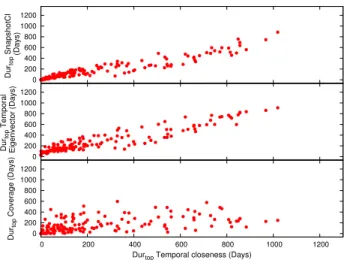
Despite these differences, one can see on Figure 10 that the four methods tend to perceive similarly the global importance of nodes; the difference between the four ap-proaches therefore lies mainly in how they evaluate unim-portant nodes, as well as the nodes of average importance.

0 0.5 1 1.5 2 2.5 3 0 0.5 1 1.5 2 2.5 3 Dur bot (Hours)

Durtop(Hours)

Temporal Eigenvector 0 0.5 1 1.5 2 2.5 3 Dur bot (Hours) SnapshotCl 0 0.5 1 1.5 2 2.5 3 Dur bot (Hours) Temporal closeness

Fig. 11: DurT opv.s. DurBot. For RollerNet dataset.

Interestingly, these observations are completely different for RollerNet. In this dataset, one can see in Figure 11 that no node spends time in the top (or bottom) region more than half of the total duration, whatever the method used (except for one node that is almost always in the bottom region). Besides, when comparing the global importance attributed to nodes by different methods (evaluated by

DurT op, Figure 12), one can see that the correlation between

temporal closeness and the other methods is not very strong and is even anti correlated with temporal eigenvector. All these observations are consistent with the fact that, in this dataset, there is no meaningful notion of global importance. We claim that this is due to the very dense (both temporally and structurally) nature of this dataset.

The Twitter dataset is also interesting as it combines the

0 0.5 1 1.5 2 Dur top SnapshotCl (Days) 0 0.5 1 1.5 2 0 0.5 1 1.5 2 Dur top Temporal Eigenvector (Days)

Durtop Temporal closeness (Days)

Fig. 12: Temporal closeness v.s. other methods. For the RollerNet dataset. 0 5 10 15 20 25 0 5 10 15 20 25 Dur bot (Days)

Durtop(Days)

Temporal Eigenvector 0 5 10 15 20 25 Dur bot (Days) SnapshotCl 0 5 10 15 20 25 Dur bot (Days) Temporal closeness

Fig. 13: DurT opv.s. DurBot. For Twitter dataset.

0 2 4 6 8 10 12 0 5 10 15 20 25 Dur top SnapshotCl (Days)

Dur_top Temporal closeness (Days)

Fig. 14: DurT opv.s. DurT op. For the Twitter dataset.

behaviours previously seen in Enron for the four methods.

Figure 13 shows that the comparison between Durtop and

Durbotis similar to what we observed on Enron, and even

more extreme: for snapshotCl, points are all situated on the line y = T − x (where T stands for the total duration), meaning that at all times, any node is either in the top or the bottom region, but never in-between. Behaviours are more nuanced for the temporal closeness and, for temporal eigen-vector, all the nodes have very similar values. This is similar to what we observed for Enron, but far more extreme. However, in contrast with Enron, the global importance (i.e.

0 0.2 0.4 0.6 0.8 1 0 0.2 0.4 0.6 0.8 1

Average Closeness (Normalized by

maximum)

Dur_top (Normalized by maximum) Enron RollerNet Twitter

Fig. 15: Durtopv.s. average temporal closeness.

the Durtopvalue) attributed by temporal closeness is not at

all correlated to the one attributed by the other methods (see

Figure 145_).

Finally, we study the results obtained for coverage cen-trality for the Enron dataset. We observe that coverage is close to snapshotCl in the sense that all nodes are always either in the top or in the bottom region (Figure 9, bottom right). However, as pointed out before, coverage does not capture the same notion of importance as temporal close-ness, which can be seen by comparing the correlation

be-tween the DurT opvalues (Figure 10 bottom). The elements

provided in this study do not allow to conclude on the reasons of this divergence and we leave this question for further studies.

7

DISCUSSION

In this paper, we considered four centrality methods that quantify the time-evolution of nodes’ importance. For the comparison of these methods, we performed several steps. This included ranking the nodes with respect to their cen-trality values, as well as computing a global duration that represents a node’s global importance. Some papers [20] propose the study of the average over time of centrality rather than its evolution. They consider that this single value is representative of the node’s complete evolution during a dataset.

To assess this claim, we propose to analyze the

correla-tion between Durtop and the average temporal closeness.

Figure 15 presents such a correlation for the three datasets. In the case of Enron and RollerNet, these values seem corre-lated (particularly for RollerNet). However, the correlation is very low for Twitter: some nodes have a high average

temporal closeness yet a low Durtop, and conversely. We

argue that the average temporal closeness is not represen-tative as it does not give each instant an equal amount of importance. As we saw, a node can have an extremely high temporal closeness at a single instant (and therefore a high average temporal closeness) even though it may have a very low activity (and hence, a very low closeness) in the rest of

the dataset. However, the Durtop value considers that all

instants have an equal importance.

To study the snapshotCl method, we had to choose a value for the snapshot duration. As explained in Section 5, we chose the value that gave a good compromise between a low loss of temporal information and a sufficiently high

5. we only present the correlation between temporal closeness and snaphsotCl as the plot obtained for temporal eigenvector is very similar.

0 200 400 600 800 1000 1200 0 200 400 600 800 1000 1200 Dur top (SnapshotCl)

1 day 1 week 2 weeks 1 month

0 0.5 1 1.5 2 0 0.5 1 1.5 2 Dur top (SnapshotCl) 30 seconds 1 minute 2 minutes 4 minutes 0 2 4 6 8 10 12 0 5 10 15 20 25 Dur top (SnapshotCl)

Dur_top (Temporal closeness) 1 hour 2 hours

3 hours 12 hours

Fig. 16: Durtopfor snapshotCl v.s. Durtopfor temporal

closeness for different snapshot sizes. Top: Enron; Middle: Rollernet; Bottom: Twitter.

number of active nodes in each snapshot, so that it contains enough information. In order to check whether this has an impact on our observations, we present in Figure 16 the

correlation between the Durtopvalues of temporal closeness

and the one of snapshotCl for different snapshot durations and for the three datasets we studied.

We observe few differences. The main difference is that for Enron, a snapshot duration significantly shorter than the one we studied in the rest of the paper (1 day) leads

to a somewhat smaller Durtop value for all nodes. This is

consistent with the fact that the snapshotCl method tends to detect the times at which the nodes are active: by reducing the snapshot duration, the relative number of snapshots at which any given node is active diminishes, hence a decrease

in the Durtop value and a corresponding increase in the

Durbot value. Note that this does not affect the general

shape of the plot, and that the Durtopvalues attributed by

temporal closenes and snapshotCl are still correlated. We study more in depth the impact of the snapshot duration in the supplementary material, and confirm that the observations made here are general and do not depend on the chosen snapshot duration.

We proposed in this paper a methodology to compare the four methods and better understand the difference be-tween each method on different datasets of different nature.

Our observations can be summarized as follows:

1) different centralities have different results; a node

closeness and irrelevant by the coverage centrality;

2) different datasets have different properties

regard-ing nodes’ importance; for one dataset, the im-portance of all nodes fluctuates extremely rapidly between high and low values; it is meaningless in this case to state that one node is more important than others, except for a very limited time span; in other datasets however, we find that some nodes are consistently important for the whole network time span;

3) a node can be inactive (i.e. not have any links) yet

be highly important since it can be a waiting point in an important temporal path between two nodes;

4) nodes can be globally important while having a low

global average centrality; average centrality gives a high significance to periods with very high temporal closeness (which correspond in general to highly active periods for the considered node).

Following those observations, we can draw a couple of conclusions regarding how to compare the different metrics. In particular, observation 3 above leads to the conclusion that snaphsotCl is unable to relate a temporary inactive node to its future connections. Therefore, it does a poor job in quantifying the importance of a node as a relay for future communication. Another conclusion drawn from the present study is that, although interesting, temporal eigenvector is less accurate than temporal closeness and coverage centrality to measure the importance of a node, as it considers path that can go backwards in time.

Our work opens the way to several interesting perspec-tives. First, the choice of several datasets stemming from very different contexts strengthens the conclusions drawn from this study. We would like to apply our approach to more datasets. For the time being, we were only able to apply the coverage centrality method to one dataset due to computational reasons. Thus, we are unable to understand completely the difference between the temporal closeness and the coverage centrality. Finding a way to speed up the coverage centrality computation, or approximate the results, would therefore allow a better understanding of this method.

Another way to address this question consists in ob-taining datasets in which the ground truth about nodes’ importance is known, or where it can be measured using an orthogonal approach. To that regards, one interesting approach could be to relate the findings provided in the present study to a practical investigation of the importance of the nodes in the network. To do so, one could for instance remove (a set of) nodes detected as important for the network by the different metrics and analyze how it im-pacts the properties of the structure in terms of information diffusion. Although very interesting, we claim that such an investigation deserves a complete and independent study that we leave for future work.

Our study of the temporal closeness centrality relies on a parameter I. Indeed, for computation reasons, instead of computing the temporal closeness for every time instant, we compute it only every I seconds. Though the values obtained in this way are exact, this may induce small

in-accuracies, mainly on the obtained values for Durtop and

Durbot: indeed, the ranking of nodes is (exactly) known for

points spaced I seconds from each other, and each point at which the rank is in the top or bottom region contributes

I seconds to Durtop or Durbot. This is an approximation

of the ideal case in which I is equal to the lowest time resolution in the dataset. The value we selected for I in the study corresponds to the median of inter-link duration (i.e. the time separating two consecutive links) for each dataset. Although we are confident that the choice of this value has little impact on the conclusions drawn in the present study, a more in-depth study of the impact of I would surely be interesting. In particular, the value of I has a strong impact on the running time of the temporal closeness computation. Being able to identify low values of I that still give relevant information would allow to run the computations much faster, and hence tackle much larger datasets.

In this paper we studied the time evolution of the importance of nodes. This topic is closely linked to the question of detecting important changes, either in the network as a whole or in the behavior of specific nodes. Some pa-pers [8], [28] study the importance of specific time instants and/or quantify the change in nodes’ importance. An in-depth study of the link between these two questions would lead to very interesting insights, for instance on questions such as: are the changes in the importance of time instants reflected in the importance of nodes at these instants? if so, do these changes correspond to a global increase/decrease of node importance, or are they triggered by a sudden increase/decrease of the importance of one (or a few) major nodes?

Finally, another interesting direction would be to de-sign or use models for temporal networks that generate artificial temporal networks in which nodes’ importance is controlled.

ACKNOWLEDGEMENTS

This work is funded in part by the European Commission H2020 FETPROACT 2016-2017 program under grant 732942 (ODYCCEUS), by the ANR (French National Agency of Research) under grant ANR-15-CE38-0001 (AlgoDiv), by the Ile-de-France Region and its program FUI21 under grant 16010629 (iTRAC).

REFERENCES

[1] Alex Bavelas. Communication patterns in task-oriented groups. The Journal of the Acoustical Society of America, 22(6):725–730, 1950. [2] Linton C Freeman. A set of measures of centrality based on

betweenness. Sociometry, pages 35–41, 1977.

[3] Leo Katz. A new status index derived from sociometric analysis. Psychometrika, 18(1):39–43, 1953.

[4] Phillip Bonacich. Power and centrality: A family of measures. American Journal of Sociology, 92(5):1170–1182, 1987.

[5] Mark Newman. Networks: an introduction. Oxford university press, 2010.

[6] Miray Kas, Kathleen M. Carley, and L.R. Carley. Incremental closeness centrality for dynamically changing social networks. In IEEE/ACM International Conference on Advances in Social Networks Analysis and Mining (ASONAM), pages 1250–1258. IEEE, 1013. [7] S. Uddin, M. Piraveenan, K. S. K. Chung, and L. Hossain.

Topo-logical analysis of longitudinal networks. In 2013 46th Hawaii International Conference on System Sciences, pages 3931–3940, Jan 2013.

[8] Shahadat Uddin, Arif Khan, and Mahendra Piraveenan. A set of measures to quantify the dynamicity of longitudinal social networks. Complexity, 21(6):309–320, 2016.

[9] Dan Braha and Yaneer Bar-Yam. Time-dependent complex net-works: dynamic centrality, dynamic motifs, and cycles of social interaction. In Adaptive networks: Theory, models and applications, pages 38–50. Springer, 2008.

[10] John Tang, Mirco Musolesi, Cecilia Mascolo, Vito Latora, and Vincenzo Nicosia. Analysing information flows and key mediators through temporal centrality metrics. In Proceedings of the 3rd Workshop on Social Network Systems, SNS ’10, pages 3:1–3:6, New York, NY, USA, 2010. ACM.

[11] B.-M. Bui-Xuan, A. Ferreira, and A. Jarry. Computing shortest, fastest, and foremost journeys in dynamic networks. International Journal of Foundations of Computer Science, 14(2):267–285, November 2003.

[12] Raj Kumar Pan and Jari Saram¨aki. Path lengths, correlations, and centrality in temporal networks. Physical Review E, 84(1):016105, July 2011.

[13] John Whitbeck, Marcelo Dias de Amorim, Vania Conan, and Jean-Loup Guillaume. Temporal reachability graphs. In MOBICOM’12, pages 377–388, 2012.

[14] Vincenzo Nicosia, John Tang, Cecilia Mascolo, Mirco Musolesi, Giovanni Russo, and Vito Latora. Graph metrics for temporal networks. In Temporal networks, pages 15–40. Springer, 2013. [15] Ingo Scholtes, Nicolas Wider, and Antonios Garas. Higher-order

aggregate networks in the analysis of temporal networks: path structures and centralities. The European Physical Journal B, 89(3):61, 2016.

[16] Ingo Scholtes, Nicolas Wider, Ren´e Pfitzner, Antonios Garas, Clau-dio J Tessone, and Frank Schweitzer. Causality-driven slow-down and speed-up of diffusion in non-markovian temporal networks. Nature communications, 5:5024, 2014.

[17] Taro Takaguchi, Yosuke Yano, and Yuichi Yoshida. Coverage centralities for temporal networks. The European Physical Journal B, 89(2):35, 2016.

[18] Enrico Ser-Giacomi, Ruggero Vasile, Emilio Hern´andez-Garc´ıa, and Crist ´obal L ´opez. Most probable paths in temporal weighted networks: An application to ocean transport. Physical review E, 92(1):012818, 2015.

[19] David A. Shamma, Lyndon Kennedy, and Elizabeth F. Churchill. Tweet the debates: Understanding community annotation of un-collected sources. In Proceedings of the First SIGMM Workshop on Social Media, WSM ’09, pages 3–10, New York, NY, USA, 2009. ACM.

[20] Hyoungshick Kim and Ross Anderson. Temporal node centrality in complex networks. Physical Review E, 85:1–8, 2012.

[21] Ahmad Alsayed and Desmond J Higham. Betweenness in time dependent networks. Chaos, Solitons & Fractals, 72:35–48, 2015. [22] Matthew J Williams and Mirco Musolesi. Spatio-temporal

net-works: reachability, centrality and robustness. Royal Society open science, 3(6):160196, 2016.

[23] Peter Laflin, Alexander V. Mantzaris, Fiona Ainley, Amanda Ot-ley, Peter Grindrod, and Desmond J. Higham. Discovering and validating influence in a dynamic online social network. Social Network Analysis and Mining, 3(4):1311–1323, October 2013. [24] Selena Praprotnik and Vladimir Batagelj. Spectral centrality

measures in temporal networks. Ars Mathematica Contemporanea, 11(1):11–33, 2015.

[25] Kristina Lerman, Rumi Ghosh, and Jeon Hyung Kang. Centrality metric for dynamic networks. In Proceedings of the Eighth Workshop on Mining and Learning with Graphs - MLG ’10, pages 70–77, New York, New York, USA, July 2010. ACM Press.

[26] Caterina Fenu and Desmond J Higham. Block matrix formulations for evolving networks. SIAM Journal on Matrix Analysis and Applications, 38(2):343–360, 2017.

[27] Dane Taylor, Sean A. Myers, Aaron Clauset, Mason A. Porter, and Peter J. Mucha. Eigenvector-based centrality measures for temporal networks. Multiscale Modeling & Simulation, 15(1):537– 574, 2017.

[28] Eduardo C Costa, Alex B Vieira, Klaus Wehmuth, Artur Ziviani, and Ana Paula Couto Da Silva. Time centrality in dynamic com-plex networks. Advances in Comcom-plex Systems, 18(07n08):1550023, 2015.

[29] Cl´emence Magnien and Fabien Tarissan. Time evolution of the importance of nodes in dynamic networks. In Proceedings of the International Symposium on Foundations and Applications of Big Data

Analytics (FAB), in conjunction with ASONAM, 2015., FAB ’15, pages 1200–1207, New York, NY, USA, 2015. ACM.

[30] Source code for the temporal centrality metrics. https://bitbucket. org/complexnetworks/closeness centrality marwan.

[31] Jitesh Shetty and Jafar Adibi. Discovering important nodes through graph entropy the case of Enron email database. In Proceedings of the 3rd international workshop on Link discovery -LinkKDD ’05, pages 74–81. ACM Press, August 2005.

[32] Radosław Michalski, Sebastian Palus, and Przemysław Kazienko. Matching organizational structure and social network extracted from email communication. In Lecture Notes in Business Information Processing, volume 87, pages 197–206. Springer Berlin Heidelberg, 2011.

[33] Pierre Ugo Tournoux, J´er´emie Leguay, Marcelo Dias de Amorim, Farid Benbadis, Vania Conan, and John Whitbeck. The Accordion Phenomenon: Analysis, Characterization, and Impact on DTN Routing. In Proceedings of the 28rd Annual Joint Conference of the IEEE Computer and Communications Societies (INFOCOM), pages 1116–1124. IEEE, 2009.

[34] Bimal Viswanath, Alan Mislove, Meeyoung Cha, and Krishna P Gummadi. On the evolution of user interaction in facebook. In Proceedings of the 2nd ACM workshop on Online social networks, pages 37–42. ACM, 2009.

[35] R. Sulo, T. Berger-Wolf, and R. Grossman. Meaningful selection of temporal resolution for dynamic networks. In Proceedings of the Eighth Workshop on Mining and Learning with Graphs, 2010. [36] S. Uddin, N. Choudhury, S. M. Farhad, and M. T. Rahman.

The optimal window size for analysing longitudinal networks. Scientific Reports, 7(1):13389, 2017.

[37] Yannick L´eo, Christophe Crespelle, and Eric Fleury. Non-altering time scales for aggregation of dynamic networks into series of graphs. In International Conference on emerging Networking EXperi-ments and Technologies (CONEXT), 2015.

Marwan Ghanem is a Ph.D. candidate at the Computer Science laboratory LIP6 (Sorbonne Universit ´e/CNRS). He received his Master of Science degree in Computer Science from Uni-versity Pierre and Marie Curie in 2015. His re-search area is the study of real complex net-works and he focuses in particular on analysing the importance of their nodes.

Cl ´emence Magnien is a senior researcher at CNRS and member of the LIP6 lab (Sorbonne Universit ´e/CNRS). She completed her PhD in computer science from ´Ecole Polytechnique in 2003, and joined LIP6 in 2007.

Her research area is the study of large graphs occurring in practice, both in computer science but but also coming from other contexts, like social or biological networks.

Fabien Tarissan is a permanent researcher at CNRS and member of the laboratory ISP at ENS Paris-Saclay. He was previously an associate professor at Sorbonne Universit ´e from 2009 to 2015. His work mainly concerns the analysis and modeling of large networks encountered in practice. His approach consists in proposing new theoretical tools in order to identify non-trivial properties of these networks and to define new models able to capture these properties.

Supplementary material

F

In this supplementary material we study more in depth the impact of the choice of the snapshot duration for the snapshotCl method.

For each of the datasets, we chose a range of values for the snapshot duration, some shorter and some larger than the one we have chosen for the main part of the paper. Then we make the same studies than in Section 6 of the main paper. −0.2 0 0.2 0.4 0.6 0.8 1 0 200 400 600 800 1000 1200 Kendall Correlation Duration

1 day 1 week 2 weeks 1 month

−0.2 0 0.2 0.4 0.6 0.8 1 0 0.5 1 1.5 2 2.5 3 Kendall Correlation Duration 30 seconds 1 minute 2 minutes 4 minutes −0.2 0 0.2 0.4 0.6 0.8 1 0 5 10 15 20 25 Kendall Correlation Duration 1 hour 2 hours 3 hours 12 hours

Fig. 1: Time-evolution of the Kendall-Tau correlation between temporal closeness and snapshotCl for different

snapshot sizes. Top: Enron; Middle: Rollernet; Bottom: Twitter.

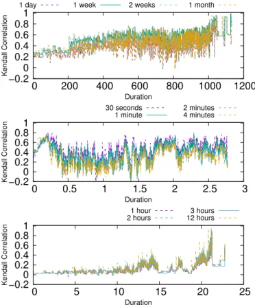
Figure 1 shows the time evolution of the Kendall-tau correlation between the rankings produced by snapshotCl and temporal closeness, for the three datasets.

We observe the same global behaviors for all snapshot durations. In particular, we still observe a global increase of the correlation for the Enron dataset, coming from the fact that, as less nodes are active at the end of the dataset, both methods tend to agree more on which nodes are important; we still observe very important fluctuations for the

Roller-Net dataset, consistent with the fact that this dataset is very dense and importance fluctuates widely from one instant to the next; and we still observe a consistently low correlation for the Twitter dataset, except at the times at which a larger fraction of nodes are active.

We now study the difference in the ranks attributed by snapshotCl and temporal closeness to each node. Figure 2 presents the inverse cumulative distribution of the differ-ence of the ranks for each node at every instant, for the three datasets.

For Rollernet and Twitter, we observe no significant differences for the different snapshot durations. For En-ron, we observe that, the higher the snapshot duration, the lower the fraction of (instant, node) pairs for which temporal closeness attributes a higher rank than snapshotCl. This is consistent with our earlier observations: snapshotCl attributes a rank of 0 during temporary inactive moments to the corresponding nodes, while temporal closeness ranks them higher. Since increasing the snapshot duration reduces the fraction of snapshots during which any given node is inactive, this induces a smaller fraction of positive rank differences.

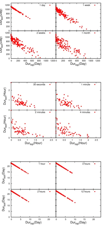
Finally, Figure 3 presents the correlations between

Durtop and Durbot values for snapshotCl, for the three

datasets. Again, for Rollernet and Twitter, we observe no significant difference: for Rollernet, we see that the values become more scattered when the snapshot duration in-creases; for Twitter however, the values are still concentrated in a single line, meaning that snapshotCl always considers a node as important or unimportant, but never places it in the middle region.

For Enron, we observe that the values become signif-icantly more scattered as the snapshot duration increases. This comes from the fact that, as the snapshot duration increases, a larger fraction of nodes become active in each snapshot, and hence not all active nodes are placed in the top region by snapshotCl. However, we still clearly observe the tendency to seldom place nodes in the middle region, characterized by a globally linear shape of the plot, even for large snapshot durations: a one month snapshot leads to approximately 36 snapshots for the whole dataset, which induces a very important loss of temporal information.

Finally, as we observed in the main text of this paper, the snapshot duration has little impact on the correlations

between the Durtop values of snapshotCl and temporal

0 0.1 0.2 0.3 0.4 0.5 0.6 0.7 0.8 0.9 1 −1 −0.5 0 0.5 1

Number (instant,nodes)

(percentage)

Ranks (Normalized by

maximum value)

Number (instant,nodes)

(percentage)

Ranks (Normalized by

maximum value)

Number (instant,nodes)

(percentage)

Ranks (Normalized by

maximum value)

Fig. 2: Inverse cumulative distribution of rank difference between Temporal Closeness and snapshotCl fir different

snapshot sizes. Top: Enron; Middle: Rollernet; Bottom: Twitter. 0 200 400 600 800 1000 1200 Dur bot (Day) 1 day 1 week 0 200 400 600 800 1000 1200 0 200 400 600 800 1000 1200 Dur bot (Day)

Dur_top(Day)

2 weeks

0 200 400 600 800 1000 1200

Dur_top(Day)

1 month 0 1 2 Dur bot (Hour) 30 seconds 1 minute 0 1 2 0 0.5 1 1.5 2 2.5 Dur bot (Hour)

Durtop(Hour)

2 minutes

0 0.5 1 1.5 2 2.5

Durtop(Hour)

4 minutes 0 5 10 15 20 Dur bot (Day) 1 hour 3 hours 0 5 10 15 20 0 5 10 15 20 Dur bot (Day)

Dur_top(Day)

2 hours

0 5 10 15 20

Dur_top(Day)

12 hours

Fig. 3: Durtopv.s. Durbotfor different snapshot sizes. Top: