Fourier transform rheology as a tool to determine the fatigue behavior of polymers

(1)

© Valerian Hirschberg, 2019

Fourier Transform Rheology as a Tool to Determine the

Fatigue Behavior of Polymers

Thèse

Valerian Hirschberg

Doctorat en génie chimique

Philosophiæ doctor (Ph. D.)

(2)

i

Fourier Transform Rheology as a Tool to

Determine the Fatigue Behavior of Polymers

Valerian Hirschberg

Doctorat en génie chimique

Philosophiae doctor (Ph.D.)

Directeur de recherche

Prof. Dr. Denis Rodrigue

Co-directeur de recherche

Prof. Dr. Manfred Wilhelm

(3)

(4)

iii

Résumé

Cette thèse propose un nouveau concept d'analyse, de quantification et de prédiction de la fatigue mécanique d'un polymère amorphe à l'aide d'une méthode basée sur la décomposition de la contrainte via la transformation de Fourier. En particulier, des essais de fatigue ont été réalisés sous déformation contrôlée en torsion et en tension/tension. La déformation, le couple et la force ont été enregistrés en fonction du temps et décomposés en contributions linéaires et non-linéaires, quantifiés par des harmoniques plus élevées. De plus, trois concepts ont été développés pour déterminer quantitativement le comportement mécanique des échantillons en fonction du temps. Premièrement, il a été établi que la génération de fissures macroscopiques était en corrélation avec l’augmentation soudaine de l’intensité de I2/1. Deuxièmement, une méthode directe pour prédire la durée

de vie en fatigue a été développée, basée sur le taux de changement de I3/1 par rapport au

nombre de cycle N (dI3/1/dN) avant l'apparition de la rupture. Cette prédiction s'est avérée

beaucoup plus précise que les prédictions des courbes de Wöhler puisque les corrélations présentent en moyenne des écarts-types beaucoup plus faibles (30 vs 60%). Troisièmement, un critère de fatigue basé uniquement sur la non-linéarité mécanique a été développé, appelé la non-linéarité cumulée Qf. Ce paramètre corrèle l'intégrale de la non-linéarité Q (Q

= I3/1/02) jusqu'à la rupture avec le nombre de cycles à la rupture Nf. L'écart-type de la

corrélation Qf vs Nf s'est avéré inférieur à 30%, indiquant que Qf est un critère de fatigue

plus précis que ceux couramment utilisés tels que la densité d'énergie dissipée cumulée ou la contrainte cumulée (±50%). Enfin, ces trois concepts ont été appliqués avec succès dans différentes conditions (type de déformation, plage de fréquence, amplitude de déformation) et différents polymères tels que le polystyrène (PS), le polyméthylméthacrylate (PMMA), le styrène acrylonitrile (SAN) et le polytertbutylméthylacrylate (PtBMA).

(5)

iv

Abstract

This thesis proposes a new framework to analyse, quantify and predict the mechanical fatigue of amorphous polymer using a method based on the decomposition of the stress response via Fourier transform. In particular, fatigue tests were performed under strain controlled torsion and tension/tension deformation and the time data of the strain, torque and force were recorded and decomposed into linear and nonlinear contributions via higher harmonics. In particular, three concepts have been developed to quantitatively determine the time behavior of the samples. Firstly, the generation of macroscopic cracks was found to correlate with sudden increases in the I2/1 intensity. Secondly, an on-line method to

predict the fatigue lifetime was developed, based on the rate of change of I3/1 with respect

to the cycle number N (dI3/1/dN) before the onset of failure. This prediction was found to be

more precise than Wöhler curves predictions since the correlations have on average much lower standard deviations (30 vs. 60%). Thirdly, a fatigue criterion solely based on mechanical nonlinearity was developed: the cumulative nonlinearity Qf. This parameter

correlates the integral of the nonlinearity Q (Q = I3/1/02) until failure with the number of

cycles to failure Nf. The standard deviation of the Qf vs. Nf correlation was found to be less

than 30%, indicating that Qf is a more precise fatigue criterion than commonly used ones

such as the cumulative dissipated energy density or the cumulative stress (±50%). Finally, these three concepts were successfully applied on different conditions (type of deformation, range of frequency, deformation amplitude) and polymers such as polystyrene (PS),

polymethylmethacrylate (PMMA), styrene acrylonitrile (SAN) and

(6)

v

List of Tables

Table 1: Molecular properties of the synthetized PS. ... 52 Table 2: Molecular characteristics of the PS with a broad and bimodal MWD. ... 52 Table 3: The measured number of cycles to failure (Nf) for tests at 0 = 0.7% and ω1/2π = 1 Hz, the rate of change of G', G'' and I3/1 and the calculated fatigue lifetimes via Eq. (41) - (43), as well as their average value. The closest prediction to the experimental value is underlined. ... 72 Table 4: The coefficient of determination r2_{, the pre-factors AW (Eq. (57)) and AQ (Eq. (62))} as well as their standard deviation for the correlations of Wf and Qf with Nf. ... 99 Table 5: The proportionality factors AWöhler, AI3/1 and AQ (Eq. (53), (68) and (70)) for the investigated polymers and geometries, as well as their standard deviations in absolute value and percent for easier comparison. The lowest standard deviations are marked in bold. ... 122

(12)

xi

List of Figures

Figure 1: Spectacular cases of failure: the Tacoma Narrows bridge due to strong winds (left) and the break-up of a newly-constructed ship after releasing from the shipyard (right) [Elliot, 1940; Parker, 1957]. ... 2 Figure 2: Typical G' and G'' behavior during a strain sweep test in the linear (SOAS) and nonlinear (LAOS) regime of a polylactic acid/nanocrystal composite (PLA2002D, Mn = 12.5 kg/mol) at ω1/2π = 1 Hz and T = 165°C, according to [Hyun, 2002]. ... 10 Figure 3: Fourier spectrum of the stress response of a polylactic acid/nanocrystal composite (PLA2002D, Mn = 12.5 kg/mol) at γ0 = 268%, ω1/2π = 1 Hz and T = 165°C. The signal to noise (S/N) ratio is in the range of 100000:1. ... 11 Figure 4: Typical response for the third harmonic (I3/1) intensity as a function of the applied strain amplitude (γ0), showing the behavior in SAOS and LAOS of a polylactic acid/(treated) nanocrystal composite (PLA2002D, Mn = 12.5 kg/mol) at ω1/2π = 1 Hz and T = 165°C. . 13 Figure 5: Typical behavior of the stress response of a strain controlled fatigue test and its corresponding hysteresis loops/Lissajous curves. ... 15 Figure 6: Schematic representation of a Wöhler curve with the three typical regimes: low and high cycle fatigue, followed by the fatigue limit. ... 16 Figure 7: Storage modulus (E') and Nonlinear Viscoelastic Parameter (NVP) as a function of time for three different loading modes of a glass fiber/Nylon6 (GF/Ny6) sample:

tension/tension (empty circle), tension/compression (full circle) and

compression/compression (empty square) at ω1/2π = 11 Hz and T = 303 K [Liang, 1996]. ... 19 Figure 8: The (normalized) decrease of G' against the (normalized) increase in I3/1 until a macroscopic crack occurred in polystyrene [Hirschberg, 2017]. ... 21 Figure 9: Storage modulus (G’) as well as I2/1 and I3/1 intensity as a function of the number of cycles (N). The I2/1 intensity increases substantially (over a factor of ten) when a macroscopic crack occurs in the sample (between N = 40 and N = 60 cycles) [Hirschberg, 2017]. ... 21 Figure 10: The second (I2) and third harmonic (I3) as a function of the number of cycles for a rubber at different strain amplitude (15-35%). The values are not normalized to the fundamental harmonic (I1). The author labeled I2 as the first and I3 as the second (higher) harmonics. Adapted from [Lacroix, 2004]. ... 22 Figure 11: Reproducibility of fatigue experiments at γ0 = 15% showing the absolute values of the higher harmonics at the beginning of the test and their trends as a function of the

(13)

xii

number of cycles. The author labeled I2 as the first and I3 as the second (higher) harmonics. Adapted from [Lacroix, 2004]. ... 23 Figure 12: Schematic overview of the objectives of the thesis. ... 25 Figure 13: Typical results for solid samples in oscillatory shear tests [Hirschberg, 2015]. a) Lissajous (stress-strain) curve of a solid PS-PI-PS triblock copolymer sample (MW = 153 kg/mol, polydispersity index (PDI) = 1.06) at ω1/2π = 1 Hz and room temperature in the linear regime (γ0 = 0.0027) and b) the FT spectrum of the stress. c) Lissajous (stress-strain) curve of the same PS-PI-PS triblock copolymer in the nonlinear regime (γ0 = 0.05). The corresponding FT spectrum of the stress in d) contains odd higher harmonics; the even harmonics are within the noise level. In the linear regime, only the peak at the fundamental frequency appears, whereas in the nonlinear regime higher harmonics up to the 13th_can be detected. ... 33 Figure 14: Typical FT spectrum of the stress response of the first 15 cycles after adjusting of a fatigue test with constant strain amplitude γ0 = 0.012. The excitation frequency is ω1/2π = 0.5 Hz. The signal to noise ratio (S/N ratio) is about 1x105_{... 35} Figure 15: Storage modulus (G’)and the intensities of the higher harmonics (I2/1 and I3/1) during a fatigue test at ω1/2π = 1 Hz and γ0 = 0.012 (left) or 0.014 (right), and room temperature (RT). The pictures below are taken from a video of the fatigue test and failure of the sample as labelled in the plot a) above. ... 36 Figure 16: The first derivative of the storage modulus G’ as a functionof the number of cycles N (dG’/dN) for the PS data of Figure 15 (γ0 = 0.012, ω1/2π = 1 Hz). The dashed line indicates the occurrence of the first macroscopic crack, corresponding to pictures a) and b) in Figure 15. ... 37 Figure 17: The Lissajous (strain/stress) curves of two nonlinear stress signals. The first Lissajous curve (I3/1 = 0.022) represents the beginning of a fatigue test on PS as reported in Figure 15 (dashed line), while for the second one, I3/1 increased by 45% (I3/1 = 0.0319, full line) which was found as a typical increase during a fatigue test until a macroscopic crack occurs. ... 39 Figure 18: The intensity of I2/1 as a function of the number of cycles N at ω1/2π = 1 Hz and a) γ0 = 0.01 and b) γ0 = 0.012. Three tests were conducted at both strain amplitudes. In a) macroscopic cracks occur after about 2200 cycles (black line), 1900 (red) and 3100 (blue), in b) after 1600 cycles (black line), 1400 (red) and 2800 (blue). At about the same time than the macroscopic cracks occur, the intensity of I2/1 increases drastically. ... 40 Figure 19: Typical behavior of the storage modulus (G’)and the intensities of the higher harmonics (I2/1 and I3/1) during a fatigue test of a notched PS sample at ω1/2π = 2 Hz and γ0 = 0.012. The images taken from the video belong to the label in the plot above to show when changes occur in the sample. ... 42

(14)

xiii

Figure 20: The values of G’ and I3/1 (red line) normalized by their initial values at the beginning of the test as a function of the number of cycles. The box indicates the region where no macroscopic crack can be seen. ... 43 Figure 21: Relative values of the elastic shear modulus as a function of the relative values of the third harmonic when the first macroscopic crack occurs. ... 44 Figure 22: Experimental setup used for the fatigue measurements. ... 46 Figure 23: G’ (a) and G’’ (b) as a function of the strain amplitude (ω1/2π = 1 Hz, RT) for the PS listed in Table 1 (low PDI). ... 53 Figure 24: I3/1 as a function of strain amplitude (ω1/2π = 1 Hz, RT) for the PS samples listed in Table 1 (low PDI). For each strain amplitude, 15 cycles were performed. ... 54 Figure 25: Number of cycles to failure (Nf) as a function of the strain amplitude (γ0) for low PDI polystyrene. ... 55 Figure 26: Value of the parameter A in Eq. (35) as a function of the weight average molecular weight for low PDI PS (see Table 1). The lines represent the correlations given by Eq. (36) and (37). ... 56 Figure 27: Values of the parameter A in Eq. (35) as a function of: a) Mw and b) Mn. The lines represent the correlations given by Eq. (36) and (37). ... 57 Figure 28: Normalized elastic modulus (G’/G’0) a) and relative third harmonics intensity (I3/1/(I3/1)0) b) as a function of the number of cycles for the different low PDI PS investigated (γ0 = 2%, ω1/2π = 1 Hz, RT). ... 58 Figure 29: Normalized elastic modulus (G’/G’0) a) and relative third harmonics intensity (I3/1/(I3/1)0)) b) as a function of the number of cycles for the different broad and bimodal MWD PS (γ0 = 2%, ω1/2π = 1 Hz, RT). ... 59 Figure 30: The linear parameters (G’ and G’’) as well as the nonlinear parameters (I2/1 and I3/1) during a fatigue test of PS200k (γ0 = 2%, ω1/2π = 1 Hz, RT). An increase of I2/1 is found while the crack propagates. ... 61 Figure 31: The number of cycles to the occurrence of a macroscopic crack as a function of: a) Mw and b) Mn. (γ0 = 2%, ω1/2π = 1 Hz, RT). The lines represent the correlations given by Eq. (36) and (39). ... 62 Figure 32: The Wöhler curve of the tests at ω1/2π = 0.5 Hz (green triangle), 1 Hz (black star), 2 Hz (pink circle) and 5 Hz (orange square). ... 69 Figure 33: Typical evolution of the three mechanical parameters (G’, G’’ and I3/1) as a function of the number of cycles (N). The curves can be divided into three regimes: after an initial phase (regime I, up to NII cycles), the three parameters linearly de/increase with the number of cycles (regime II, up to NIII cycles), before failure onset occurs (regime III). In regime II, the slope of the three parameters were calculated (dG’/dN, dG’’/dN and d3/1/dN). The tests were performed at ω1/2π=1 Hz, γ0 = 0.5% and RT. ... 70

(15)

xiv

Figure 34: Fatigue lifetime (Nf) of the PS samples as a function of the absolute values of the rates of change of: a) G’, b) G’’ and c) I3/1 calculated in regime II. The full lines represent the correlations of Eq. (41) - (43), while the dashed lines represent a 30% deviation. ... 74 Figure 35: Typical evolution of the three mechanical parameters (G’, G’’ and I3/1) as a function of the number of cycles (N) for PMMA (a) and SAN (b) samples. The curves can be divided into three regimes: after an initial phase (regime I, up to NII cycles), the three parameters de-/increase linearly with the number of cycles (regime II, up to NIII cycles), before failure onset occurs (regime III). In regime II, the slopes of the three parameters were calculated (dG’/dN, dG’’/dN and d3/1/dN). The tests were performed at ω1/2π = 1 Hz, γ0 = 0.5% and RT. ... 76 Figure 36: Fatigue lifetime (Nf) of PMMA samples as a function of the absolute values of the rates of change of G’, G’’ and I3/1 calculated in regime II. The full lines represent the correlations of Eq. (44)- (46), while the dashed lines represent a 30% deviation. ... 77 Figure 37: Fatigue lifetime (Nf) of SAN samples as a function of the absolute values of the rates of change of G’, G’’ and I3/1 calculated in regime II. The full lines represent the correlations of Eq. (47) - (49), while the dashed lines represent a 30% deviation. ... 78 Figure 38: The linear parameters G' and G'' as well as the nonlinear ones I3/1 and I2/1 as a function of the number of cycles during a fatigue test of PS (ω1/2π = 1 Hz, γ0 = 0.8%). At the transition from regime II to regime III, the I2/1 intensity first decreases before it increases drastically by nearly two orders in magnitude until failure. To better see these changes, a logarithmic axis is employed, in comparison to linear ones for I3/1 above. ... 81 Figure 39: Wöhler curves of PMMA (left) and SAN (right) at ω1/2π = 1 Hz. ... 81 Figure 40: NII/Nf (black square) and NIII/Nf (red circle) as a function of the applied strain amplitude for: a) PS, b) PMMA and c) SAN. ... 82 Figure 41: Normalized number of cycles to the de-/increase of G'00, G’’00 and I3/1,00 by the corresponding prefactor AF of Eq. (41) - (49). ... 82 Figure 42: The parameter Q as a function of cycle number for PS98k (full red line). The dashed surface represents the cumulative nonlinearity Qf. ... 90 Figure 43: The cumulative nonlinearity until failure as a function of the number of cycles to failure for selected polymers: PS98k (black square), PMMA (red circle), SAN (green diamond) and PtBMA (blue triangle). ... 92 Figure 44: Cumulative nonlinearity as a function of the number of cycles to failure for different frequencies (0.5, 1, 2 and 5 Hz) for different PS molecular weights (Mn = 82, 98, 125, 190, 380 and 840 kg/mol). ... 94 Figure 45: Prefactor AQ of the correlations between the cumulative nonlinearity with the number of cycles (Eq.(62)) as a function of the number average molecular weight Mn (a))

(16)

xv

and the prefactor of the Wöhler curves (fatigue resistance, Eq.(53), AWöhler) for PS samples with different molecular weight. ... 95 Figure 46: Cumulative stress density σf and dissipated energy density Wf as a function of the number of cycles to failure for the investigated polymers PS98k, PMMA, SAN and PtBMA a) and b), for PS98k at different frequencies c) and d), and for PS with different molecular weights e) and f).This analysis is analog to Figure 43 and Figure 44 for Qf. ... 96 Figure 47: The different pre-factors (AW and Aσ) for the correlations between the cumulative stress and dissipated energy density with the number of cycle to failure as a function of the number average molecular weight Mn (a) and of the pre-factor of the Wöhler curves (b), fatigue ressistance, AWöhler) for PS samples with different molecular weights. ... 97 Figure 48: Stress controlled cycling of PMMA, PS200k and PS400k as a function of the deformation a) and a magnification of the small deformation zone is given in b). The curves reveal that the three materials deform plastically, as even after the first cycle a zero stress does not correspond to a zero strain. ... 110 Figure 49: Fourier spectra of the force response of dumbbell samples of PMMA on the Electro Force 3300-AT from BOSE (a), ω1/2π = 5 Hz, ε0 = 0.8%, R = 0.1) and on the Acumen 3 from MTS (b), ω1/2π = 5 Hz, ε0 = 0.8%, R = 0.1). For the signal from the BOSE, beside the fundamental harmonic at ω1/2π = 5 Hz, especially odd higher harmonics at ω1/2π = 15, 25, 35 Hz, etc. can be seen. The signal to noise ratio is in the range of 1:104_{to 1:10}5_for both machines. ... 110 Figure 50: The normalized complex modulus ׀E*׀ and the higher harmonics intensities (I2/1 and I3/1) as a function of the applied strain amplitude ε0 as precited by the Neo-Hooke law. The complex modulus ׀E*׀ decreases as a function of the strain amplitude, whereas the I2/1 intensity increases and the I3/1 intensity increases at strain amplitudes above 0.05 for the resolution used. The fatigue tests were performed at strain amplitudes smaller 0.01, indicated by the dashed purple line. ... 111 Figure 51: Typical behavior of the complex modulus ׀E*׀ (black line), the average stress E0 (green line) and the nonlinear parameters I3/1 (red line) and I2/1 (blue line) as a function of the cycle number for a dumbbell sample of PMMA (a), ω1/2π = 5 Hz, ε0 = 0.3%, R = 0.1 and PS200k (b), ω1/2π = 5 Hz, ε0 = 0.3%, R = 0.1. The solid black line through the I3/1 data represents the rate of change of I3/1 (dI3/1/dN), the E0 data of the PMMA tests shown is the fitted exponential decrease to smoothen the data. ... 113 Figure 52: The logarithm of the I3/1 increase as a function of the E0 decrease in regime I ((I3/1)II/(I3/1)0 vs. E0/EII) for PMMA (a) and PS200k (b). For PMMA different loading ratios R = 0.1 (black square), 0.3 (red circle) and 0.5 (blue triangle) were investigated and for PS200k R = 0.1. The tests were performed at ω1/2π = 5 Hz. The black lines represent the best fits

(17)

xvi

with a slope of -2.7 for PMMA and -9.3 for PS200k, showing much higher changes in I3/1 for PS200k than for PMMA for similar changes in E0. ... 114 Figure 53: The number of cycles to failure (Nf) as a function of the rate of change of I3/1 (dI3/1/dN) in regime II, for dumbbell samples of PMMA (a) and PS200k (b) at ω1/2π = 5 Hz. For PMMA different deformation ratios were investigated: R = 0.1 (black square), 0.3 (red circle) and 0.5 (blue triangle) and for PS200k: R = 0.1. The black lines represent the best fit for R = 0.1 with slopes of -1.3. ... 115 Figure 54: The cumulative nonlinearity (Qf) as a function of Nf for dumbbell samples of PMMA (a) and PS200k (b) at ω1/2π = 5 Hz. For PMMA different deformation ratios were investigated: R = 0.1 (black square), 0.3 (red circle) and 0.5 (blue triangle), for PS200k: R = 0.1. The black lines represent the best fit for R = 0.1, with slopes of 1.75. ... 115 Figure 55: The evolution of ׀E*׀, I2/1 and I3/1 as a function of the cycle number for notched PMMA samples (ω1/2π = 5 Hz, ɛ0 = 0.35% and 0.2%) at different deformation ratios: a),b) R = 0.1, c),d) R = 0.3, e) R = 0.5 and f) R = 0.7. ... 117 Figure 56: The evolution of ׀E*׀, I2/1 and I3/1 as a function of the cycle number for a notched PS200k (ε0 = 0.3%) and PS400k (ε0 = 0.35%) sample (ω1/2π = 5 Hz, R = 0.3). ... 118 Figure 57: Micrographs of PMMA, PS200k and PS400k (ω1/2π = 5 Hz, ε0 = 0.2%, 0.3% and 0.35%, R = 0.3) broken surfaces revealing two zones of different crack propagation rates via a rough (the river patterns, fast crack growth with plastic deformation) and a smooth surface area, containing (for PMMA) striations (slow crack growth, brittle failure). ... 119 Figure 58: Correlations between Qf, dI3/1/dN and Nf for notched rectangular PS200k (black square) and PS400k (red circle) samples. The black lines represent the best fit. ... 121

(18)

xvii

Abbreviations

DE Dissipated Energy during one cycle

FT Fourier transform

LAOS Large amplitude oscillatory shear

MAOS Medium amplitude oscillatory shear

PDI Polydispersity index

PI Polyisoprene

PLA Polylactic acid

PMMA Polymethylmethacrylate

PS Polystyrene

PtBMA Polytertbuthylmethacrylate

S-N curve Stress-number of cycles to failure curve S/N ratio Signal to noise ratio

SAN Styrene-acrylonitrile

SAOS Small amplitude oscillatory shear

SI Polystyrene-polyisoprene diblock copolymer

(19)

xviii

Symbols

A Surface

AQ Proportionality constant of the cumulative nonlinearity vs. number of cycles

correlation

AI3/1 Proportionality constant of the dI3/1/dN vs. number of cycles correlation

AWöhler Proportionality constant of the Wöhler curve

B Prefactor of the Wöhler correlation

C Exponent of the Wöhler correlation

δ1 Phase angle of the fundamental harmonic

δ2 Phase angle of the second harmonic

δ3 Phase angle of the third harmonic

δ4 Phase angle of the fourth harmonic

δ5 Phase angle of the fifth harmonic

dI3/1/dN Rate of change of I3/1 in regime II

abs(dG’/dN) Rate of change of G’ in regime II abs(dG’’/dN) Rate of change of G” in regime II

EDiss Dissipated energy during one cycle

E’ Storage modulus (elongation)

E’’ Loss modulus (elongation)

׀E*׀ Complex modulus (elongation)

E0 Relaxation modulus (elongation)

ε Strain (elongation)

ε0 Strain amplitude (elongation)

(20)

xix

 Strain (torsion)

0 Strain amplitude (torsion)

+ Clockwise strain

- Counter-clockwise strain

G’ Storage modulus (shear)

G’’ Loss modulus (shear)

G* Complex modulus

I2/1 Ratio of the second harmonic normalized by the fundamental

I3/1 Ratio of the third harmonic normalized by the fundamental

I4/1 Ratio of the fourth harmonic normalized by the fundamental

I5/1 Ratio of the fifth harmonic normalized by the fundamental

Mn Number average molecular weight

Mw Weight average molecular weight

η Viscosity

NI Cycle number at the transition from regime I to regime II

NII Cycle number at the transition from regime II to regime III

Nf Number of cycles to failure

NVP Nonlinear viscoelastic parameter

ω Angular frequency

ω1 Angular frequency of the deformation

Q Ratio of the intensity of the third harmonic over the square of the strain amplitude

Q0 Parameter of the intrinsic nonlinearity

Qf Cumulative nonlinearity

(21)

xx

RDEC Ratio of Dissipated Energy Change

σ Stress

s(t) Time signal

S(ω) Signal in the frequency domain after FT

t Time

Tg Glass transition temperature

T/T Tension/tension

Wdiss Dissipated Energy Density

Wf Cumulative Dissipated Energy Density

(22)

xxi

(23)

xxii

Acknowledgement

Most importantly, I would like to thank everyone who helped me to complete my Ph.D. thesis successfully. Firstly, I would like to thank my supervisor Prof. Denis Rodrigue for the highly interesting and scientifically challenging subject of my thesis, his guidance and support, the very fruitful and challenging discussions over the past three years, and last but not least the financial support which allowed me to focus on my research. Secondly, I would like to thank my co-supervisor Prof. Manfred Wilhelm for the time I could spend in his laboratories, the fruitful and challenging discussions and the financial support. Thirdly, I would like to thank all my friends and colleagues at ULaval and KIT, with special thanks to Jian Zhang (ULaval), Dr. Dimitri Merger (KIT), Lorenz Faust (KIT) and Dr. Mahdi Abbasi (KIT), as well as Mr. Yann Giroux (ULaval) and Mr. Daniel Zimmermann (KIT) for the excellent technical support. Fourthly, I would like to thank Prof. Florian Lacroix and Prof. Stéphane Méo for the opportunity to stay in their Institute at the Université de Tours in summer 2018, the support over there and the discussions. Furthermore, I would like to thank NSERC, CREPEC, CQMF and CERMA for financial and technical support, as well as providing the equipment.

Finally, I would like to thank my family, my parents, my brother Leander and my girlfriend Shan Lyu for their unconditional love and support.

(24)

xxiii

Foreword

The work presented hare was done under the supervision of Prof. Denis Rodrigue at Université Laval in Quebec City/Canada and the co-supervision of Prof. Manfred Wilhelm at the Karlsruhe Institute of Technology (KIT) in Karlsruhe/Germany. The mechanical testing in torsion was mostly done at ULaval, whereas the synthesis of polymer model systems was done in the laboratories at KIT. The tests in tension/tension where mostly done during a research stay at the Université de Tours in France, funded by a “MITACS Globalink Award” scholarship.

This thesis contains nine chapters, one is a book chapter, three are published articles and two are submitted articles.

Chapter 2

Hirschberg V, Wilhelm M, Rodrigue D. Fatigue behavior of polystyrene (PS) analyzed from the Fourier transform (FT) of stress response: First evidence of I2/1(N) and I3/1(N) as new fingerprints. Polym Testing 2017, 60, 343-350.

Chapter 3

Hirschberg V, Schwab L, Cziep M, Wilhelm M, Rodrigue D. Influence of molecular properties on the mechanical fatigue of polystyrene (PS) analyzed via Wöhler curves and Fourier Transform rheology. Polymer 2018, 138, 1-7.

Chapter 4

Hirschberg V, Wilhelm M, Rodrigue D. Fatigue life prediction via the time-dependent evolution of linear and nonlinear mechanical parameters determined via Fourier transform of the stress. J Appl Polym Sci 2018, 46634.

Chapter 5

Hirschberg V, Wilhelm M, Rodrigue D. Cumulative nonlinearity as a criterion to quantify mechanical fatigue. Subm. to Int J Fatigue, 2018.

Chapter 6

Hirschberg V, Lacroix F, Wilhelm M, Rodrigue D. Fatigue and fracture analysis via Fourier transform of the stress of brittle polymers in tension/tension.Subm. to Mech Mater, 2019.

(25)

xxiv

My contribution as the first author includes the planning, the measurements, the analysis and the interpretation of the data obtained, as well as the writing of the first version of the articles. My supervisors, Prof. Rodrigue and Prof. Wilhelm, as co-authors of these articles, supervised the work, helped with highly fruitful and challenging discussions and revised the written articles.

The results were published in scientific journals, but also presented at several conferences as oral presentation and as poster, as well as institute/group/center seminars at ULaval and KIT. Two invited seminars were also presented, the references are listed below. The poster presented at the “90th_{Annual Meeting of the Society of Rheology” in Houston (USA)} won the 2nd_{prize in the Ph.D. student/Post-doc poster competition.}

Conference Contributions:

1.

V. Hirschberg, M. Wilhelm, D. Rodrigue.

“Fatigue fingerprints via Fourier transform of the stress.”

90th_{Annual Meeting of the Society of Rheology, Houston, USA, 14-18.10.2018, paper SG17.} 2.

“Fatigue analysis via Fourier transform of the stress.”

90th_{Annual Meeting of the Society of Rheology, Houston, USA, 14-18.10.2018, poster} PO102.

3.

“Fatigue Analysis and Prediction via Fourier Transform of the Stress. “

12th_{International Fatigue Congress, Poitiers (France), 27.05.-01.06.2018, paper PS18,} #00375.

4.

“Fingerprints of mechanical fatigue via Fourier transform of the stress response with application on polystyrene (PS)”.

(26)

xxv 5.

M. Wilhelm, S. Nie, L. Schwab, V. Hirschberg, M. Cziep, J. Lacayo-Pineda. “FT-Rheology on Rubber Materials”.

TA-Instruments Conference. Würzburg (Ger), 28.04.2017. 6.

D. Rodrigue, V. Hirschberg, M. Wilhelm.

“The effect of testing conditions on the mechanical properties of polymers during fatigue testing”.

88th_{Annual meeting of the Society of Rheology. Tampa (USA), 12-16.02.2017.} 7.

“Fatigue Behavior of Polylactic Acid (PLA) analyzed from the Fourier Transform (FT) of their Stress Response”. Proceedings of the XVIIth_{International Congress on Rheology (ICR2016).} Kyoto (JP), 8-13.08.2016.

8.

“New Fingerprints of Fatigue: Nonlinear Parameters I2/1 and I3/1(t) of Fourier Transform (FT) of the Stress Response with Application on Polystyrene (PS) and High Impact Polystyrene (HIPS)”.

PolyMerTec Conference. Merseburg (Ger), 15-17.07.2016.

Invited Seminars

1.

Valerian Hirschberg, Manfred Wilhelm, Denis Rodrigue.

“Fatigue Analysis of Polymers via Fourier Transform of the Stress”

Seminar of ‘GRK 2078’, Institute of Engineering Mechanics, Karlsruhe Institute of Technology, invited by Prof. Thomas Böhlke, 31.07.2018.

2.

Valerian Hirschberg, Manfred Wilhelm, Denis Rodrigue.

“Fatigue Analysis and Prediction via Fourier Transform of the Stress”

(27)

xxvi

Furthermore, during my stays in the laboratories of Prof. Wilhelm at the KIT, the effect of PS/PI copolymerisation on the fatigue properties and the evolution of the higher harmonics was systematically investigated. Therefore, model systems of PS-PI-PS (SIS) and PS-PI (SI) with different molecular weight and PI content were synthesized via anionic polymerisation. In total over 25 samples were synthesized, but as the characterisation is not yet finished and published, this work is not further discussed here.

(28)

1

General introduction

The world plastic production has risen rapidly since the 1950s from about 1.5 Mt/a to 335 Mt/a in 2016 and is expected to grow to over 1800 Mt/y in 2050, the so-called success story of plastics. About one third of the world production of plastics is used for packaging, another third in buildings such as pavements, windows and piping. The last third includes industrial components such as cars, toys and furniture [Andrady, 2009]. In several applications, plastics are replacing common materials. Plastics offer various advantages against common materials such as metals, wood and ceramics: low density, resistance again corrosion, wide range of processing possibilities and low costs (~2 US$/kg) for the commodity plastics such as polyethylene (PE), polyvinyl chloride (PVC) or polypropylene (PP). Furthermore, polymers are viscoelastic. As a result, the stress response (force normalized by the loaded area) contains both an elastic and a viscous part, characterized as the storage modulus (E’) and loss (E’’) moduli in tension or G’ and G’’ in shear/torsion. This viscoelastic behavior results in a nonlinear stress response under large load/deformation. Nonlinearity means in this context that the stress response is no longer directly proportional to the applied load/deformation.

Due to the lower mechanical strength of neat polymers compared with metals (in machines) or concrete (in construction), polymers are seldom used as load bearing components. Polymers are typically used for all kind of applications where the properties of polymers are superior to other materials but are still exposed to a mechanical stress. For example, in pavement, floor-covering, windows or piping, often also in combination with physical aging (influence of temperature/weather).

With important advancements in the technology of 3D printing not only small and low-cost objects, but also complex structures up to complete houses, can be printed with high quality and speed. Polymers and polymer-based materials can be used due to their rheological and mechanical properties. The increase of high-quality polymer-based products also underlines the demand for an in-depth understanding of the mechanical long-term properties during application, thus mechanical fatigue.

The failure of a material under a repetitive load or deformation is called mechanical fatigue [Andrew, 1995]. The phenomenon of mechanical fatigue is a long-term process due to a recurring deformation or load and is in general hardly detectable unless visible cracks or the catastrophic event itself (failure) occurs. Fatigue is one of the main limitations with respect to lifetime of the application of every solid part and responsible for about 90% of all mechanical service failures [Campbell, 2008]. One of the underlying processes resulting in

(29)

2

accidents such as the collapse of bridges or dams, train accidents, plane crashes or the failure of machines and devices is mechanical fatigue. Prominent accidents due to fatigue are the collapse of the Tacoma Narrows bridge or the Liberty ships (Figure 1). In fact, most accidents and catastrophic events, which are not directly related to human failure, are related to mechanical fatigue. For our daily life, the safe use without the fear of failure is of fundamental interest and consequently attracted the attention of scientists and engineers from the beginning of the industrial revolution. Additionally, the economical losses due to mechanical fatigue are reported to be around 4% of the Gross Domestic Product (GDP) in the United States [Stephens, 2000], corresponding (for 2016) to a loss of 742 billion US$. The world loss is consequently about of 3.22 trillion USD (2017, using the world gross product), which is roughly double the GNP of Canada in 2017, underlining the whole extent of damage of mechanical fatigue.

Figure 1: Spectacular cases of failure: the Tacoma Narrows bridge due to strong winds (left) and the break-up of a newly-constructed ship after releasing from the shipyard (right) [Elliot, 1940; Parker, 1957].

Since the beginning of the industrial revolution around 1800, the then-new phenomenon of cyclic mechanical fatigue of metal in construction and machines, such as bridges and railways, has been observed and investigated. Firstly, publications on the systematic analysis of fatigue can be found from the 1830th_{on by English, French and German} engineers. The most well-known name related to fatigue at that time is August Wöhler who first published the concept of the analysis of the number of (sinusoidal) cycles (N) to failure of metal dumbbell samples as a function of the applied stress amplitude (S), nowadays known as Wöhler or S-N curve (“Über Versuche zur Ermittlung der Festigkeit von Achsen”, 1867, in (more ancient) German, “On fatigue experiments of axel”) [Wöhler, 1867]. Wöhler curves are still the state-of-the-art approach to characterize and quantify the fatigue resistance of a material, connecting the fundamental parameters in mechanical fatigue

(30)

3

testing: the number of cycles to failure (N) and the stress (S) or deformation amplitude. The main challenge of Wöhler curves and mechanical fatigue testing in general is the probabilistic nature of fatigue, thus the poor reproducibility of the number of cycles to failure for the same material under the exact same testing conditions. The standard deviations of Wöhler curves are typically far above 100% for metals and typically above 50% for polymers. The range of lifetime for metallic samples under the same measurement conditions is reported as up to several decades and in an older extreme case, with up to four orders of magnitude. Due to the highly probabilistic nature of mechanical fatigue, intensive research in this field is necessary to improve the understanding of fatigue and to protect human and environment from the catastrophic event of failure.

An in-depth understanding of fatigue needs to investigate the different stages of fatigue and fracture. In general, three different regimes can be observed: crack initiation, crack propagation and fast crack growth/catastrophic failure. Before crack initiation, no changes due to damage are visible. So, several experimental, empirical and analytical approaches were developed to better detect, quantify and predict those evolutions and events during mechanical fatigue. Methods based on external devices such as video or thermal cameras, or on the material parameters themselves, for example via an analysis of the dissipated energy during one cycle or in total up to failure, were proposed. The fatigue analysis in deformation/strain controlled tests, providing more information about the current state of fatigue, without using additional devices, as e.g. a camera, are based on the analysis of the stress response of the material.

From rheology, different techniques and frameworks exist to investigate and quantify nonlinear contributions in the stress, the strain or strain rate in the time domain. In the strain/strain rate domain, hysteresis loops or so-called Lissajous curves, can be used to quantify changes from the linear response via Chebyshev coefficients for example. In the time domain, the stress can be decomposed into linear and nonlinear contributions via Fourier transform with high sensitivity; i.e. the so-called FT-rheology. The excitation mode of choice is nowadays sinusoidal and can be performed on the experimental devices with a high signal to noise (S/N) ratio, typically in the range of 105_{:1 and nonlinear contributions} in the rage of 10-3_{to 10}-4_{can be measured and reproducible at small strain amplitudes.} Rheology investigates the linear and nonlinear mechanical material properties as a function of the deformation or deformation rate, but mechanical fatigue of solids is typically not investigated. However, in mechanical fatigue testing, only few papers can be found dealing with the analysis of the stress and none applying the technique of FT -rheology. An example from fatigue testing is the so-called nonlinear viscoelastic parameter (NVP), calculating the intensity of the sum of higher stress harmonics over the fundamental, analog to the total

(31)

4

harmonic distortion for sound systems. This parameter was investigated for fatigue tests in tension and compression and found to increase at failure. With the knowledge and understanding from FT-rheology, the drawbacks of the NVP as well as its limited predictive power are easily understandable. Firstly, it does not analyze odd and even higher harmonics separately, so no difference is made between the higher harmonics representing the geometric symmetry (odd higher harmonics) and the asymmetric contributions (even higher harmonics) of the stress response. For an undamaged sample, noise is summed up via the even or the even and odd higher harmonics, depending on the material, the deformation direction and the applied stress/strain amplitude.

This thesis investigates a multidisciplinary topic at the interface between polymer science, rheology and mechanical engineering. The work deals with the investigation, quantification and prediction of mechanical fatigue and failure via the linear and nonlinear contributions of the materials stress response. Mechanical fatigue and fracture itself are nonlinear processes, so the expectation is high to find typical patterns and fingerprints in the stress.

(32)

5

Chapter 1 1.1 Literature overview

Dynamic Rheology and Mechanics of Polymers in their Solid

State

Hirschberg V, Wilhelm M, Rodrigue D. Book chapter submitted to: Llewellyn, P. Rheology of Polymer Blends and Nanocomposites: Theory, Modelling and Applications. Elsevier.

Résumé

Ce chapitre présente une revue de littérature sur les propriétés rhéologiques et mécaniques dynamiques des polymères à l'état solide. En présence de grandes déformations, la contrainte des polymères n’est plus linéaire et différentes techniques ont été proposées pour analyser le comportement non-linéaire de ces matériaux. Les techniques et théories actuelles sont présentées, mais la rhéologie à transformation de Fourier (FT) est mise en détail.

De plus, ce chapitre traite de la fatigue mécanique des polymères. Premièrement, les concepts de base sont présentés en utilisant la représentation bien connue des courbes de Wöhler du nombre de cycles à la rupture en fonction de l'amplitude de la contrainte (contrainte imposée) ou de la déformation (déformation imposée). Deuxièmement, une discussion est faite sur les différentes approches pour suivre les changements des propriétés des matériaux au cours des essais, par exemple: l'énergie dissipée, le paramètre viscoélastique non-linéaire et l'analyse des harmoniques supérieures de la réponse aux contraintes via FT. Enfin, les tendances actuelles des recherches sont présentées.

(33)

6

Abstract

This chapter presents an overview of the dynamic rheological and mechanical properties of polymers in their solid state. Under large deformation, the material response of polymers is no longer linear viscoelastic and different techniques have been proposed to analyze the nonlinear behavior of these materials. The current techniques and theories are presented, but Fourier transform (FT) rheology is more detailed.

Furthermore, this chapter deals with the mechanical fatigue of polymers. The basic concepts are presented first using the well-known Wöhler curves representation of the number of cycles to failure as a function of the applied stress (stress controlled) or strain (strain controlled) amplitude. Secondly, a discussion is made on the different approaches to follow the material properties changes during testing/application such as: the dissipated energy function, the nonlinear viscoelastic parameter and the analysis of higher harmonics of the stress response via FT. Finally, the current investigation trends are presented. Keywords: Dynamic rheology, Nonlinearity, Fourier transform rheology, mechanical fatigue.

(34)

7

1.1.1 Introduction

The world plastic production rapidly increased since the 1950s from 1.5 to more than 300 Mt/y today (2018). About one third of the world plastics production is used for packaging, another third in buildings (pavements, windows and piping), while the last third includes industrial components (automotive, toys and furniture) [Andrady, 2009]. In several applications, plastic parts replace common materials (metals, wood and ceramics) since they provide various advantages such as low density, corrosion resistance, a wide range of processing possibilities to allow basically all shapes of the final part in combination with low costs, especially for the so-called commodity plastics like polyethylene and polypropylene.

But polymers are viscoelastic materials and show, in the melt and solid state, a nonlinear response when the deformation exceeds a certain threshold. Viscoelasticity implies that the stress response contains both an elastic and a viscous part characterized by the storage E’ and loss E’’ moduli in tension, or G’ and G’’ in shear/torsion. Nonlinearity means that the stress response is no longer proportional to the load/deformation. Under simple shear, the viscosity might de-/increase as a function of the applied shear rate after a constant plateau value at small deformations/rates [Bird, 1987; Carreau, 1997]. Under oscillatory shear, the stress response becomes nonlinear, so the parameters G, E,  and tan(δ) are not constant anymore, but depend on the applied conditions. During oscillatory shear higher harmonics (through FT) can be detected, see below [Giacomin, 1993; Wilhelm, 2002].

The rheological properties of melts are of high importance for polymer processing. So, it is important to know the viscosity at a given temperature and shear rate, as well as how it is influenced by their changes in processes like extrusion, injection molding, etc.

One of the main limitations with respect to the application of every solid part is its lifetime. In particular, the failure of a solid material under a repetitive load is called mechanical fatigue [Andrew, 1995], which is responsible for about 90% of all the mechanical service failures [Campbell, 2008]. For our daily life, safe use without the fear of failure is of fundamental interest.

It is a challenge to predict the long-term performance of a material under a load. The first publications on the systematic analysis of fatigue can be found from the 1830s by English, French and German engineers, investigating the then-new phenomenon of cyclic fatigue of metal in construction and machines like railways. The most well-known name related to fatigue at that time is August Wöhler (“Versuche über die Festigkeit der Eisenbahnwagenachsen” (“Study on the Stability of Railroad Vehicle Axes”) [Wöhler, 1867]), who analyzed the number of (sinusoidal) cycles (N) to failure of a metal dumbbell sample as a function of the applied stress amplitude (S), nowadays known as Wöhler or S-N curve. However, Wöhler curves is an old characterization tool for mechanical fatigue under

(35)

8

dynamic loading but is still state-of-the-art since it represents the simplest way to characterize and quantify the fatigue resistance of a material. The main drawback of Wöhler curves are their typically large standard deviations [Bathias, 2013], and the resulting limited meaning for an individual sample. The deformation mode of choice is nowadays sinusoidal and can be performed with a low signal to noise (S/N) ratio.

The mechanical fatigue testing of polymers must also take a polymer specific property into account: their viscoelasticity and their nonlinearity at large strain amplitudes [Sauer, 1980]. Recent methods of fatigue analysis in deformation/strain controlled tests, providing more information about the current state of fatigue, without using additional devices (camera), are based on the stress response analysis of the material. The stress response can be analyzed in strain/strain rate or time domains. In the strain domain (hysteresis loops or so-called Lissajous curves), although (large) changes can be seen by the naked eye, they can hardly be quantified. In the time domain, different parameters and analysis methods exist based on a FT of the stress. As an example, the nonlinear viscoelastic parameter (NVP) was proposed which represents the sum of the stress higher harmonics over the fundamental, analog to the total harmonic distortion for sound systems. Another approach is to analyze the higher harmonics separately which has the advantage, especially in torsion/shear, of separating between the material dependent parameters (higher odd harmonics) and parameters related to asymmetry in the stress response (higher even harmonics). These concepts are described next.

1.1.2 Viscoelasticity of solid polymers

1.1.2.1 Viscoelasticity of polymers

Rheology investigates the flow behavior of materials under deformation. The basic parameters are therefore the normalized deformation, the strain () and the resistance force (F) of the material, typically normalized by the loaded surface (A) to get a system independent quantity, which is the stress (σ):

𝜎 =𝐹 𝐴

(1) Static and dynamic deformations can be applied to a material, but the focus here is on dynamic (sinusoidal) deformations.

1.1.2.2 Linear viscoelasticity

The typical models to describe elasticity and viscosity are the ideal elastic solid and the ideal viscous fluid, represented by a spring and dashpot (mechanical analogy). The ideal elastic solid can be described by Hooke’s law with the modulus G as the proportional constant between strain and stress. Newton’s law describes the stress for an ideal viscous fluid, with the viscosity η as the proportional factor between shear rate and stress.

(36)

9

𝜎 = 𝐺𝛾 (2)

𝜎 = 𝜂𝛾̇ (3)

Models to describe the rheological and mechanical behavior of viscoelastic materials combine typically spring and dashpot (Hooke’s and Newton’s law) respectively, in different numbers and ways. The simplest viscoelastic solid model is the Kelvin-Voigt model, combining spring and dashpot in parallel. On the other hand, the Maxwell model combines spring and dashpot in series for a viscoelastic liquid. More advanced models are also available (Burgers, Jeffreys, etc.).

Under small amplitude oscillatory shear (SAOS), the stress response is linear with the strain amplitude; i.e. if the strain is sinusoidal, the stress is sinusoidal as well but with a lag. A complex notation can be used, so the strain is written as (according to Euler’s rule):

𝛾 = 𝑖𝛾0𝑒𝑖𝜔1𝑡 (4)

𝜎 = 𝑖𝐼1𝑒𝑖(𝜔1𝑡+𝛿1) (5)

Consequently, the stress response under oscillatory shear can be completely mathematically described by a complex function with the magnitude I1 and phase angle δ1.

The magnitude I1 divided by the strain amplitude is the complex modulus (G*), and together

with the phase angle, form a set to describe in a complex plane the real (G’) and imaginary part (G’’). This regime is called the linear or SAOS regime. In the linear regime, the storage and loss moduli are independent of the applied strain amplitude and provide rheological parameters to completely characterize a material in a meaningful way.

1.1.2.3 Nonlinear viscoelasticity

In the nonlinear regime, under the conditions of large amplitude oscillatory shear (LAOS), the above statements do not hold anymore. Consequently, G’ and G’’ depend on the applied strain amplitude. Figure 2 presents an example for G’ and G’’ as a function of the strain amplitude. For small strain amplitudes, G’ and G’’ are constant and independent of the strain amplitude, but they can increase/decrease for larger strain amplitudes, so:

𝐺 = 𝐺(𝛾0) ≠constant (6)

For fluids, four main types of G’ and G’’ behavior as a function of strain amplitude were described [Hyun, 2002]. When G’ and G’’ decrease with increasing strain, strain softening (Type I) occurs, while the reverse is called strain hardening (Type II). If G’ decreases but G’’ increases before decreasing, leading to a weak strain overshoot (“Payne effect” for filled rubbers) this is associated to Type III. Finally, when both parameters increase before they decrease with a strong strain overshoot, Type IV is obtained. However, mixed behaviors out of these four main types have been reported.

(37)

10

Figure 2: Typical G' and G'' behavior during a strain sweep test in the linear (SOAS) and nonlinear (LAOS) regime of a polylactic acid/nanocrystal composite (PLA2002D, Mn = 12.5 kg/mol) at ω1/2π =

1 Hz and T = 165°C, according to [Hyun, 2002].

A stress versus strain curve (so-called Lissajous curve) can be plotted for each cycle. The shape of a Lissajous curve is a straight line for an ideal elastic body and a circle for an ideal viscous one [Larson, 2006]. Consequently, the shape of the Lissajous curve can be correlated to the material viscoelasticity. It shows if a viscous or elastic behavior dominates and if the stress response is linear or not. However, Lissajous curves can hardly detect small nonlinear contributions and are unable to quantify them.

1.1.2.4 Large amplitude oscillatory shear (LAOS)

1.1.2.4.1 Fourier Transform

The FT is a reversible mathematical function decomposing a signal into a sum of sine and cosine functions or (using Euler’s approach) a sum of exponentials [Brigham, 1974]. It calculates the periodic contributions of a time signal, displaying their amplitudes and phases (or in a complex plane as the real and imaginary parts) as a function of frequency. The FT of any real- or complex-time signal s(t), or frequency dependent spectrum S(ω) (inverse FT), are typically defined as:

𝑆(𝜔) = ∫ 𝑠(𝑡) 𝑒

−𝑖𝜔𝑡

𝑑𝑡

∾ −∾ (7) 𝑠(𝑡) = 1 2𝜋∫ 𝑆(𝜔)𝑒 𝑖𝜔𝑡_𝑑𝜔 ∞ −∞ (8)

(38)

11

Moreover, the FT is an orthogonal (linear) transform. Consequently, the sum of two functions in the time domain correspond to their sum in the frequency domain [Bracewell, 1986].

𝑎𝑠(𝑡) + 𝑏𝑔(𝑡) ↔ 𝑎𝑆(𝜔) + 𝑏𝐺(𝜔) (9)

Since the FT transposes a real (time) signal into a complex (frequency) signal, a FT spectrum contains real and imaginary parts. In the complex plane, each signal can be considered as a vector from the origin with a magnitude Iω and a phase φ(ω).

1.1.2.5 Fourier transform rheology

The stress response becomes nonlinear under LAOS conditions [Giacomin, 1993]. Nonlinearity means in this context that the stress and strain/strain rate are not directly proportional to each other.

𝜎 ≠ 𝛾, 𝛾̇ (10)

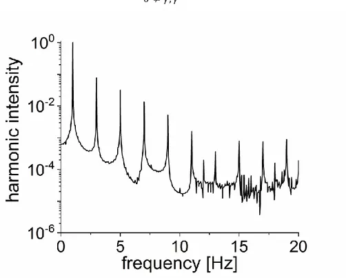
Figure 3: Fourier spectrum of the stress response of a polylactic acid/nanocrystal composite (PLA2002D, Mn = 12.5 kg/mol) at 0 = 268%, ω1/2π = 1 Hz and T = 165°C. The signal to noise (S/N) ratio is in the

range of 100000:1.

From an experimental point of view, this means that the modulus and viscosity are affected by the testing conditions (strain/strain rate, see Figure 2). The linear parameters G’ and G’’ are sufficient to describe the stress response completely in the linear case (Eq. (2-3)). However, this is not enough in the nonlinear regime, so they partially lose their (physical) meaning. Therefore, it is necessary to use a more advanced approach to completely describe

(39)

12

the stress response. Currently, the nonlinear stress response was analyzed quantitatively in the strain/strain rate [Cho, 2005; Ewoldt, 2008] or the time domain [Wilhelm, 2002; Hyun, 2011]. In the strain/strain rate domain, the corresponding Lissajous curves are decomposed into elastic and viscous moduli, by using Chebyshev polynomials for example. In the time domain, the stress signal is decomposed into a Taylor series of odd higher harmonics of the deformation frequency, using FT. This decomposition is better done in the time domain since it is easier to analyze for a time dependent process like fatigue. However, Fourier series can be converted into Chebyshev coefficients.

1.1.2.5.1 Odd higher harmonics

The FT of the nonlinear stress response only shows odd higher harmonics, as shown in a typical FT spectrum presented in Figure 3. This can be explained using the simplest nonlinear 1D scalar model for an elastic solid body, a nonlinear spring [Doetsch, 2003]. In such a model, the spring constant (which corresponds to the modulus) depends on the strain:

𝜎 = 𝐺(𝛾)𝛾 (11)

Additionally, it is assumed that the modulus of the clockwise half cycle G(+_{) is equal to the}

counterclockwise cycle G(-_{), which is a reasonable assumption for isotropic materials. As a}

result, the (complex) modulus depends only on the absolute values of the strain:

𝐺(𝛾+_{) = −𝐺(𝛾}−_{) = 𝐺(|𝛾|)} ₍₁₂₎

𝜎 = 𝐺(|𝛾|)𝛾 (13)

Consequently, if the absolute value of the modulus is expanded in a Taylor series of the strain, only even powers are obtained:

𝐺(|𝛾|) = 𝐺1+ 𝑎1𝛾2+ 𝑏1𝛾4+. .. (14)

Inserting Eq. (4) and Eq. (14) in Eq. (13) gives:

𝜎 = 𝐺(|𝛾|)𝛾 = (𝐺1+ 𝑎1𝛾2+ 𝑏1𝛾4+. . . )𝛾0𝑒𝑖𝜔1𝑡 (15)

𝜎 = 𝐺1𝛾0𝑒𝑖𝜔1𝑡+ 𝑎1𝛾03𝑒3𝑖𝜔1𝑡+ 𝑏1𝛾05𝑒5𝑖𝜔1𝑡+. .. (16)

which can be rewritten as:

𝜎 = 𝐼1𝑒𝑖𝜔1𝑡+ 𝐼3𝑒3𝑖𝜔1𝑡+ 𝐼5𝑒5𝑖𝜔1𝑡+. .. (17)

To better quantify and compare a nonlinear behavior, mostly the third harmonic (I3ω1) is

considered and normalized to the fundamental harmonic (I1ω1) typically written as (I3/1).

From Eq. (16) and (17) it can be seen that the nth_{harmonic depends on the n power of the} strain amplitude and consequently the In/1 intensity depends on (0)n-1. The I3/1 intensity in

a strain sweep test, including linear and nonlinear regime, typically follow the behavior described in Figure 4 (log-log plot). Firstly, the I3/1 intensity decreases with a slope of -1,

before it increases with a slope of 2 and levels off to a constant value at very large strain amplitudes. The decrease of I3/1 with a slope of -1 (mostly in the SAOS regime) is caused by

(40)

13

the sensitivity limit of the torque transducer (Eq. (18)) [Reinheimer, 2012b]. Below the minimum instrument torque resolution, In cannot be detected and can be assumed to be

equal to noise N: 𝐼𝑛/1∼ 𝑁 𝐼1 ∼ 𝑁 𝛾0 ∼ 𝛾0−1 (18)

Figure 4: Typical response for the third harmonic (I3/1)intensity as a function of the applied strain

amplitude (0), showing the behavior in SAOS and LAOS of a polylactic acid/(treated) nanocrystal

composite (PLA2002D, Mn = 12.5 kg/mol) at ω1/2π = 1 Hz and T = 165°C.

The increasing part of the curve with a slope of 2 is also theoretically expected (Eq. (17)). However, theoretical calculations predict that I3/1 quadratically depends on the strain

amplitude even in SAOS, but its values become negligibly small (<10-4_{- 10}-5_{) [Merger, 2016].} Therefore, it is important to mention from an experimental point of view that for a given (nonlinear) viscoelastic material, the strain amplitude of the I3/1(0) minimum does not

represent the transition between SAOS and LAOS. It is an instrument related property as it depends on the signal to noise ratio (resolution) of the torque transducer, the oversampling and the sampling rate.

1.1.2.5.1.1 The intrinsic nonlinearity Q0

The nonlinear parameter I3/1 (and higher odd harmonics) quantifies the level of material

nonlinearity at a given strain amplitude. For a general material nonlinearity quantification, a measurement condition independent quantity must be used. After the minimum, the I3/1

(41)

14

intensity scales quadratically with 0 before leveling off, following a power-law relation

[Hyun, 2009; Cziep, 2016]:

𝑄 =𝐼3/1 𝛾02

(19) For each material (and temperature/frequency) Q is constant over a range of strain amplitudes and a parameter can be defined characterizing the material which is independent of the applied strain amplitude:

𝑄0= lim 𝛾0→0

𝑄 =𝐼3/1 𝛾02

(20) 1.1.2.5.2 Even higher harmonics

As described in section 1.1.2.5.1 for isotropic materials (G(+_{) = G(}-_{)), only odd higher}

harmonics should be obtained in the stress FT spectrum under LAOS conditions. However, higher even harmonics, typically with a lower intensity than the odd ones (I2/1 < I3/1, I4/1 <

I5/1, etc.), can be observed. For isotropic materials, these even higher harmonics are mostly

related to measurement artefacts on the macroscopic level, besides the error range of the experiment (lack of sensitivity), for example wall slip [Hatzikiriakos, 1991] or inertia [Atalık, 2004]. However, Sagis et al. [Sagis, 2001] theoretically predicted and experimentally showed the occurrence of even harmonics in the stress response caused by changes on a microscopic level. For demonstration purpose, they used a viscoelastic material with anisotropic rigid particles. Their main statement is that for broken shear symmetry to occur (G(+_{) ≠ G(}-_{)), odd and even harmonics are needed to completely describe the stress}

response. Moreover, Sagis et al. [Sagis, 2001] were able to theoretically and experimentally show that higher even harmonics first increase with increasing deformation, go to a maximum, and then decrease at very large strain amplitudes.

1.1.3 Mechanical fatigue

This section describes the most important approaches related to the methodology and analysis of dynamic fatigue testing. The experiments can be performed under controlled (constant) strain or stress. The main focus here is on a strain controlled approach, since it is the most used one towards continuous signal analysis. In strain controlled fatigue testing, the strain amplitude is constant, typically following a sine function. The stress response as a function of the number of cycles, can be presented by hysteresis loops/Lissajous curves as described in Figure 5. Furthermore, the strain amplitude, as well as the experimental setup/conditions (sampling rate), must be carefully chosen to completely analyze the stress signal higher harmonics during a fatigue test.

(42)

15

Figure 5: Typical behavior of the stress response of a strain controlled fatigue test and its corresponding hysteresis loops/Lissajous curves.

1.1.3.1 Different loading modes

Fatigue tests can be performed under different loading conditions like shear or torsion, tension/tension, tension/compression or three-point bending/dual cantilever. An important characteristic for the test results comparability and the higher harmonics contribution prediction is the stress ratio (R), which is defined as ratio between the minimum and maximum stress:

𝑅 = minimum stress maximum stress

(21) Under oscillatory shear and three-point bending/dual cantilever geometries, the stress ratio (R) is usually equal to -1, since it is not necessary to use a preload. This simplifies the higher harmonics analysis and interpretation since the same higher harmonics are expected as in the rheology of polymer melts under LAOS conditions. Consequently, only odd higher harmonics are expected, representing the material viscoelastic nonlinearity. In cases when the even harmonics intensity increases above the noise level during a test, this indicates that the stress signal is not symmetric anymore and could be related to the appearance of macroscopic cracks [Hirschberg, 2017].