Assembling Regions for Efficacious Aggregate Query
Processing in Wireless Sensor Networks
by
Apostolos Fertis
Diploma, Electrical and Computer Engineering (2003)
National Technical University of Athens
Submitted to the Department of Electrical Engineering and Computer Science
in partial fulfillment of the requirements of
Masters of Science in Computer Science and Engineering
at the
MASSACHUSETTS INSTITUTE OF
June 2005
TECHNOLOGY
©
Massachusetts Institute of Technology. All rights reserved.
Author...
... ...
Department of Electrical Engineering and Computer Science
_June 22, 2005
Certified by ... .)d
Karen Sollins Principal Research Scientist
· hs Supervisor
Accepted by ... - , 4 '- ' ' ' ' ', 2 ' ' . ... . ...
Arthur C. Smith Chairman, Department Committee on Graduate Students
ARCHIVES
MASSACHUSETTS INSTITUTE
IF
TFrC NiW l rvVL- AR M I
Contents
Abstract
1 Introduction
1.1 Query answering in sensor networks ... 1.2 Encouraging the cooperation among sensors ... 1.3 Protocols for improving aggregation ...
2 Background
2.1 Regions.
2.2 TAG ...
2.3 Probabilistic Query Model ...
2.4 Attempting to construct the Minimum Steiner Tree . 2.4.1 The metric Steiner tree problem ... 2.5 Building a new protocol ...
3 Classifying functions
3.1 Functions that can be divided into segments ... 3.1.1 Partitionable or decomposed functions ... 3.1.2 Monolithic functions ...
3.1.3 Fully partitionable functions ...
3.1.4 Recursive functions . . . . 3.2 Aggregate functions.
3.3 The importance of decomposing functions ... ....
3 9 11 11 12 13 15 15 18 19 21 22 23 27 27 28 28 29 30 31 31
...
...
...
...
...
...
...
...
...
...
...
...
...
...
... I ...
...
CONTENTS 4 Resource Management in Sensor Networks
4.1 The case of aggregate queries ... 4.1.1 Considering TAG performance . 4.1.2 Optimizing the aggregation tree. 4.2 Minimizing energy .
4.2.1 Analyzing the tranmission control mechanism . . . 4.3 Minimizing response time ...
4.4 Calculating the link quality metrics ... 4.5 Managing response energy and time ...
5 The protocol SYMPHONY
5.1 Computing aggregates in sensor networks ... 5.2 Definition of a region in SYMPHONY ... 5.3 Routing the information to compute aggregates . . . 5.4 Dividing the participating sensors into tiers ... 5.5 The shortest path overlay network ... 5.6 Identifying regions.
5.7 Identifying paths.
5.8 SYMPHONY's operation ... 5.9 Finding tier-is.
5.9.1 The JOINREQUEST messages ...
5.9.2 5.9.3 5.9.4 5.9.5 5.9.6 5.9.7 5.9.8 5.9.9 5.9.10 5.9.11
Information about paths maintained in sensors Keeping information about the discovery tree Using JOINJREQUEST messages to find tier-is Receiving a JOINREQUEST message ... The structure of JOINANSWER packets . . . The problem of sending a JOINREQUEST in b Paths cannot form cycles in SYMPHONY . . . Finding another path ...
Receiving JOINANSWER messages ... Finding shortest paths to the discovered tier-is
33
...
34
...
... 34
...
35
...
36
...
37
. . . 3 9...
42
...
44
45...
46
...
48
...
48
...
49
... . . . .... 50...
52
... 53...
55
...
56
...
57
...
59
...
63
...
64
...
65
... 66...
69
...
70
...
71
...
72
...
73
. o ~oth . . · . direction . .... . .. .. . .. .. 4CONTENTS
5.10 Synchronization of the finding tier-is procedures ...
5.10.1 Establishing the shortest paths ...
5.10.2 ()rganizing the formation of the discovery tree . . .
5.10.3 Structure of the FINDTIER1 packets ...
5.10.4 Structure of the FOUNDTIER1 packets . . . . 5.11 Path reinforcement ...
5.11.1 The overlay network is propagated to the root . . . 5.11.2 lDistributing reinforcement commands ...
5.11.3 Reinforcing paths . ... .
5.12 Results of SYMPHONY's operation ...
6 Evaluation of SYMPHONY
6.1 Communication cost for constructing the aggregation tree 6.2 The JOINREQUEST packets ...
6.2.1 Total number of JOINREQUEST messages sent . . 6.3 The JOINANSWER packets ...
6.4 The FINDTIER1 messages ... 6.5 The cost of FOUNDTIER1 packets ... 6.6 Calculating the cost of the reinforce packets ... 6.7 Total communication cost ...
6.8 Taking the decision of whether to form the tree ... 6.9 Techniques to minimize the cost of the aggregation tree's co 6.10 Balancing SYMPHONY's cost ...
7 Conclusions
7.1 SYMPHONY's principles.
7.2 Reducing the construction cost - A trade-7.3 SYMPHONY's contribution ... . . . . . . . . . . . . . . . . . . . . . . . . . . . . . . . . . . . . . . . . . . . . . . . . . . . . . . . . .n.t.u.t.o. . . . .. . . . . 76 76 77 77 79 82 82 82 84 86 89 89 90 91 91 92 93 94 95 96 96 98 99
...
100
...
101
...
102
A Pseudocode for SYMPHONY 103
Bibliography
5
List of Figures
2.1 Minimum Spanning Tree .
2.2 Minimum Steiner Tree ...
2.3 Depth first Euler tour traversal of the Minimum Spanning Tree ... 2.4 Depth first Hamiltonian path traversal of the Minimum Spanning Tree .
... . 21
... . 22
... . 24
... . 24
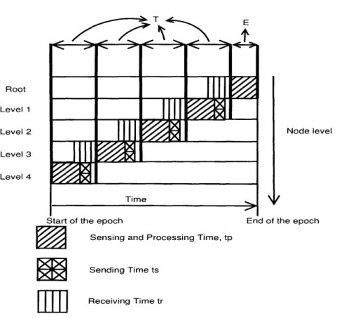
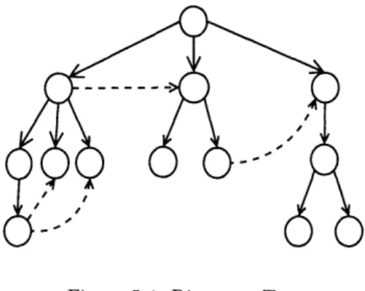
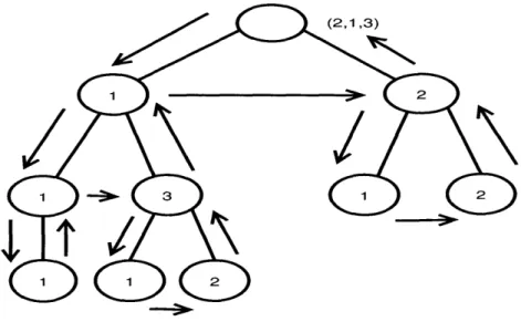
4.1 Computing aggregate for some part of the network ... 4.2 Time schedule for computing aggregates using a routing tree in TAG . 35 41 5.1 No cycles are formed in shortest path approximation graph 5.2 Identification sequences for paths that start from the origin 5.3 Identification sequences for a path that branches into a set of 5.4 Discovery Tree. 5.5 5.6 5.7 5.8 5.9 5.10 5.11 5.12 5.13 Path Tree Example ... Path costs entered in PathCost field ... A subtree of the overlay network ... Procedure of finding tier-is ... The results from finding the tier-is are propagated back . . A JOINREQUEST sent in both directions of a link .... A path cannot revisit some node ... Reconstruction of the network graph ... Reconstruction of the graph using the path tree ... 5.14 Propagation of FINDTIER1 and FOUNDTIER1 messages
...
52
...
53
f new paths ... . 54 ... 6155...
61
...
62
...
... 64
. 68...
69
...
70
...
71
...
73
. . . 74...
78
7LIST OF FIGURES
5.15 Reinforcing paths in an overlay graph ... 86
Abstract
The field of sensor networks is rapidly developing enabling us to deploy them to an unpredictable environment and draw diverse and interesting information from it. Their capabilities are improving. They can sense complicated phenomena, they take measurements for several attributes, they make numerous computations and they communicate large amounts of information.
Most sensors are battery operated and in most cases they are not easily rechargeable, as the envi-ronment in which they are located is not easily accessible. Thus, they have limited energy, which should be used to draw out as much useful information as possible. Moreover, quite often we need to receive data from a sensor network at a high rate. In order to be able to manage energy and time efficiently in sensor networks, we have to develop protocols that synchronize the cooperation among sensors and send
information to the targets as quickly as possible and with low energy consumption.
In many cases, the whole set of values that are measured is not required by the query which is submitted to the network. The query asks for an aggregate over the measurements. The propagation
of all measured values to a central computation point is resource consuming. Tiny AGgregation (TAG) provides an algorithm to compute aggregates by merging and forwarding partial results. The merging is done in the internal nodes of the routing tree that is formed.
Sometimes, the aggregation is applied over a subset of the measurements. Furthermore, the wireless links that connect the sensor nodes are not characterized by the same congestion. This fact makes the energy spent for transmission across a link varying. In addition, the use of links with high congestion in the routing tree delays the propagation of partial records to the root and thus, increases the response time. The protocol SYMPHONY provides an improvement on the TAG algorithm. It forms a Steiner tree that spans the sensors that participate in the aggregate and has cost which does not exceed the double of the optimal Steiner tree cost for the connectivity graph. The Expected Transmission Count
10 LIST OF FIGURES
(ETX) and the latency metrics are used for the links.
The communication and energy cost of forming the SYMPHONY routing tree is proved to be poly-nomial in the number of nodes. The construction cost can be reduced if the requirements for the cost in the resulting routing tree are relaxed. In any case, the use of SYMPHONY can save much energy, if the aggregate is computed in a frequent rate.
Chapter 1
Introduction
Sensor networks form an emerging technology attracting the networks community, which enables the users to acquire a huge amount of information from a rather unknown and unpredictable environment. They consist of a set of small in size and simple in construction complexity devices, which are capable of sensing various environmental attributes, implement wireless communication with radios and carry out remarkable computations. Those devices give the users the opportunity to draw detailed information about the environment in which they are placed.
1.1 Query answering in sensor networks
Sensor networks answer queries by finding the nodes which collect the relevant information and by combining their observations. This requires that data has to be propagated to the node, which will produce the answer. A sensor network is a pervasive computing environment, which has to manage its resources. Every query that is answered consumes both communication and energy resources. The communication resources refer to the bandwidth that is used for the data communication and the energy resources refer to the sum of the energy that is used to transmit the packets with this information, as well as the energy for the computation, the storage and the retrieval. The ultimate goal is to answer as many queries as possible using the fewest possible amount of resources.
The time required to get the answer to a query depends highly on the delay in the propagation of the information that it asks for. Queries which force the movement of a large amount of information may
CHAPTER 1. INTRODUCTION
wait for a long time before they start doing the computations. A significant part of the delay is due to congestion, which increases the time that is wasted in collisions. When a large number of packets needs to be transmitted, the expected total delay due to retransmissions is high. The situation deteriorates when many queries run concurrently. They increase the information load that needs to be transmitted through the network, which makes the collisions in the attempts to transmit packets more frequent, the delay big and the throughput low. This situation increases the total time to produce the response to a
query.
We assume that sensors are battery operated. The amount of consumed energy resources for a query affects the lifetime of the network, as it is difficult to recharge the batteries of the sensors. If queries quickly exhaust the energy that sensors can use, the network will stop operating early, having answered
few queries.
Every node wishes to collect information from a certain set of sensors in order to answer a query. A way to find the response to it is to propagate all the measurements needed to the node that was queried. This way leads to excessive usage of both communication and energy resources. In many cases, the total computation may be divided into parts, which can be combined to generate the final answer. Each part requires the information collected by a special set of sensors. Since every sensor has a notable computation power, certain calculations may be done in some of the nodes that collect the desired information. Such an operation requires the design of a plan that controls the cooperation of the sensors and the merging of the intermediate results.
1.2 Encouraging the cooperation among sensors
Resource management can become more efficient, if we enable the cooperation among the sensors. Such a cooperation should be based on an organized plan to ensure that the correctness of the produced results is preserved.
The Regions Project [1] provides us with an interesting and useful paradigm. In that project, the region is defined to be a set of contained members, which share some common invariants. Every query requires the measurements for some attributes. In our project here, the members of a region will be the sensors which capture those measurements. The invariant that the members of the region share is the common query, which requires their participation.
In [4], Deshpande et al. propose a Markovian probabilistic model for the attributes measured by the
1.3. PROTOCOLS FOR IMPROVING AGGREGATION
sensors. Such a n-lodel enables us to estimate the answers to some kinds of queries with certain confidence, without knowing the exact values for all the needed attributes. Such a model may be combined with the regions concept in sensor networks to reduce the answering time, as well as the cost in resources.
Ill [3], Madden et al. propose a protocol that computes aggregates in an energy efficient way. It constructs a routing tree that spans the whole network. The information is transmitted from the leaves to their parents. Every node merges the results that it received from its children with its own results and transmits a record which represents all those values to its parent. The root of the tree produces the record which represents the values from all the nodes and uses it to compute the aggregate value. The energy savings depend on the size of the transmitted record.
1.3 Protocols for improving aggregation
In this thesis we investigate the use of appropriately defined regions to support and improve query responses in such a sensor net, especially given that at least some very interesting aggregate queries can be factored, subdivided or otherwise broken into functions over smaller sets of sensors than the original query. The classification of the functions and the division into regions provides the basis for improved efficiency in the reliability and performance of sensor networks. A protocol that enables sensor networks to construct regions, maintain them and use them to produce answers to aggregate queries will be developed. The benefits of using regions in the time required to answer those queries and in resource management will be analyzed.
More specifically, we will investigate the properties of the routing or aggregate trees of TAG. We will examine how these properties affect the energy and communication cost spent to compute the aggregate values. In addition, we will investigate the effect of the aggregate tree's properties in the time required to answer the aggregate query. We will search for ways to construct aggegate trees that can compute aggregates without spending too much energy and in a small amount of time.
Furthermore, we will analyze the energy cost of constructing improved aggregation trees. This cost is going to determine the benefit from using more sophisticated algorithms in constructing those trees. This cost is going to depend on the topology of the network, but we will try to compute bounds for it that take into consideration even the more difficult cases.
The thesis is organized into the following chapters. In chapter 2, research work upon the thesis was built is presented. More specifically, the Regions project, Tiny AGgregation (TAG), a probabilistic
14 CHAPTER 1. INTRODUCTION
model for answering queries in sensor networks and an approximation algorithm for computing Steiner trees are presented. In chapter 3, we divide functions into categories according to their capability of being divided into multiple computation segments. In chapter 4, we analyze the metrics that determine the resources spent in computing aggregates. In chapter 5, we define SYMPHONY, a protocol which constructs aggregation trees for efficient computations. In chapter 6, we compute the communication cost spent in constructing the SYMPHONY aggregation tree. Finally, in chapter 7, we conclude the thesis and propose ideas for extending SYMPHONY.
Chapter 2
Background
In this thesis, we propose the idea that the existence of appropriate regions in sensor networks will improve the aggregate query processing procedure over subsets of the members of the sensor net. The queries will be answered quicker and using smaller amounts of communication and energy resources via the regions organization. The protocol that will be designed is based in existing work carried out in the field of organizing network nodes into regions, in the field of computing aggregate functions in sensor networks and in the field of computing Steiner trees over graphs.
2.1 Regions
The Regions Project introduces the idea of network regions and investigates the applications that can be implemented through them. The definition of the abstract term region, the construction of such entities and the validation of their concept are the aims of the project.
In [1], Sollins defines a region to be "a set of contained members, which share some common invariants, and a boundary, which allows us to capture the notion of actions taken when entering and leaving the region". In the sensor nets case, the invariants are the queries or functions which require the participation of the region's members. The notion of the boundary is also useful. Let us assume the generation of a query somewhere in the global network. The node where the query was originated has to send this query to a sensor, which will trigger the anwering process. The sensor node sends a packet out in the sensor network, in which it states that it requires the answer to that query. A special region for that query
CHAPTER 2. BACKGROUND
has been constructed. When the packet gets to a member of the region, it can learn where the answer that it seeks will be stored after the computation is over. Thus, once the packet crosses a boundary of this region, the procedure of finding the storage point of the answer should run. If the region has not computed the returned value of its function yet or the result that has been computed is old, the procedure of calculating the result should be triggered.
The regions definition could state that regions should have only one invariant, but sometimes, we
would like to define regions which have more than one invariant. Sensors which participate in a set of
functions and have access to the returned value of those functions are able to compute more complicated functions. These functions should be decomposed to the original set of functions. Those sensors form another region, which has more than one invariant. If we would like to define a region which requires that its members have certain values for two or more invariants, then its membership function can be the intersection of the membership functions of the regions which are defined by each of those invariants. In this case, we would have to define a merged boundary for the intersection. That is why regions are
defined to have one or more invariants.
In other cases, we do not require all invariants to be true for every member. Some nodes might
participate in the calculation of the value of one function and others might participate in the calculation of the value of another. A function subdivided in those two functions would require the union of the two
regions in order to be calculated. In this case, the union of regions is also useful.
Sollins also raises the problem of distinguishing regions in [1]. One approach is that the invariants are predefined and, in this way, the regions that are going to be formed are determined from scratch. Another approach is that a node is made a member by explicitly setting the invariants. In this case, there might be elements that meet the criteria but are not in the region.
In [1], Sollins follows the approach that it is necessary to identify the regions distinctly, which is also
followed in the sensor network regions. One way of succeeding in this is to use the sets of invariants in
order to make such a distinction. This implies that there should be a common agreement on invariant representation and that no two regions have the same set of invariants assigned to them. In this way, two statements of invariants that are not intended to be the same are distinctly represented. Moreover, a set of invariant assignments defines only one region. Such requirements ask for global coordination.
Sollins follows an alternative approach, in which each region is assigned a globally unique identifier. Any
global naming scheme will work. The sensor network regions will be assigned identification numbers. The procedure of joining a region consists of setting characteristics and introduction. The new
2.1. REGIONS
member should have the invariants corresponding to the region set to the values specified by this region. If the invariants were not true in the new member before joining the region, they have to become true. If it is assigned contradictory invariants, it will be expelled from the region. In the sensor nets case, this is straightforward. The new member is going to add the function that the region computes into the set of functions in which it participates. The joining procedure is followed by the introduction, which may be triggered either by humans or by other members of the region. The introduction ensures that the sensor which joins will be considered a member of the region, when membership functions are computed.
The ideal organization of a region implies that by being a member of the region, the sensor knows which
measurements to take, which computations to make and where to send them. Of course, this is a hard problem to solve. Furthermore, the new member may continue to take part in that region, even if the member that introduced it into the region does not belong to it any longer. The end user may decide that it wants a slight variation of the function that it asked for previously. This variation may not require all the measurements that the initial function needed. It is more efficient to change the initially constructed region than to construct a new region from scratch. So, some sensors are no longer required to be members of the region. In this case, it is simpler to modify the existing membership of a region to meet changing objectives than to create a new region. In constrast, the members that they introduced may still be in the modified region.
Regions should have the capability of re-organizing themselves internally in order to improve their behavior. Such an improvement will be triggered and may be based on size, patterns of usage, demands for performance or other costs. The re-organization can change the degree of accuracy achieved in the functions that regions implement. The size of regions' representation is crucial. If the region has a large number of members, more efficient representations are required. The sensor net regions may change their members and so, their size can fluctuate. They should be able to change their representation when their size gets over or gets under a certain critical threshold. Moreover, the sensors of a region cooperate in calculating a function following some specific organization plan. Sometimes, the conditions or the objectives change and so, a new organization plan should start being implemented.
In conclusion, the regions project plays an important role in sensor networks because it gives us a way to enable the cooperation among the sensors. It helps us dinstinguish among regions and sets the requirements, which the functions implementing the join of new members and the re-organization of the region should satisfy.
CHAPTER 2. BACKGROUND
2.2
TAG
In [3], Madden et al. propose Tiny AGgregation (TAG), an algorithm to compute aggregates over a set of attributes. The aggregates are computed using a routing tree. Every sensor that is an internal node in the routing tree aggregates the intermediate results which receives from the sensors that are its children in the routing tree. The final result is produced in the root of the tree. The aggregate function is computed using three other functions: a merging function f, an initializer i and an evaluator
e. Function f has the structure < z >= f(< x >, < y >), where < x > and < y > are multi-valued
partial state records that represent the intermediate state required to compute the aggregate over one or more values. < z > is the partial-state record which represents the intermediate state for the union of the values that < x > and < y > represent.
Madden et al. classify aggregate functions according to four dimensions. The first one is called
duplicate sensitivity. Duplicate insensitive aggregates are unaffected by duplicate readings from a
single device, whereas duplicate sensitive aggregates are going to be altered if a duplicate reading is reported. The second dimension characterizes aggregates as exemplaries or summaries. Exemplary aggregates return one or more of their values that represent the whole set. Summary aggregates compute some property of their values. The third dimension divides aggregates into monotonic and
non-monotonic ones. An aggregate is non-monotonic if for every pair of state records sl and s2, the state
record s, which results through the merging of sl and s2, satisfies e(s) > MAX(e(si), e(s2)) or e(s) <
MIN(e(si), e(s2)). The fourth dimension examines the size that is required to represent partial state
records. In distributive aggregates, the partial state is the aggregate value for the set of values that it
represents. In algebraic aggregates, the partial states are not aggregates, but they have constant size. In holistic aggregates, the size of the partial states is proportional to the number of values that they represent. In unique aggregates, the size of the partial states is proportional to the number of distinct values that belong to their partition. In context-sensitive aggregates, the size of the partial state is proportional to some property of the values in their partition.
TAG consists of two phases: a distribution phase and a collection phase. In the distribution phase, the routing tree is constructed recursively. Initially, the root of the tree, which is the sensor that is asked a query, broadcasts a message requesting the aggregation of r, the set of attributes that will participate in the aggregation. This message is propagated in the network. Each one of those messages contains the identification number of the sender, the level of the sender in the formed tree, the set of the values
2.3. PROBABILISTIC QUERY MODEL
that need to be aggregated and a time interval, which determines the time when this node requires the reception of the partial state records from its children. When a sensor receives such a message, it chooses the sender of the message to be its parent and forwards the request to aggregate r message to the rest of the network, setting the time interval to be such that its children are asked to deliver their measurements slightly before it needs to send its measurements to its parent. The collection phase is divided into epochs. In each epoch, an aggregate value is computed. Each sensor knows the time when it is supposed to capture measurements, receive the partial state records from its children, combine them to produce the partial state record corresponding to its subtree and send it to its parent from the time interval field included in the aggregate request message that it received from its parent during the distribution phase.
The production of the intermediate results, which are the partial state records corresponding to the subtrees, reduce the total amount of information that needs to be transmitted. The amount of information that should be communicated and that is saved through TAG depends on the aggregate function that is computed and on the topology of the network. If the partial state records have constant size, the total communication cost that is spent to compute an aggregate value is proportional to the number of edges of the routing tree.
2.3 Probabilistic Query Model
In [4], Deshpande et al. use a Markovian dynamic probabilistic model in order to estimate the values of the measured attributes. The model aims to encapsulate the correlation among various attributes, which makes their estimation possible with low error. More specifically, Deshpande et al. assume that the set of attributes which is under observation follows a certain joint probability distribution. In their case, Multivariate Gaussian distribution is studied but the same ideas can be applied to other distributions as well. The choice of the Multivariate Gaussian distribution is based on its generality.
The answer to a query can be computed for a given probability distribution at any time. The probability distribution determines the confidence in the answer. Some values for the attributes are known. In this particular model, this means that their probability distribution is a delta function. As the number of the attibute values which are known increases, the confidence in the answer of the query increases too. The flexibility of the model lies in the fact that even without the knowledge of the exact values for many arguments, the estimation of the final answer can be sufficient. If the goal is a desired
CHAPTER 2. BACKGROUND
confidence, an observation plan with the set of attributes that should be known with certainty should be executed. Many observation plans may achieve the desired confidence. Thus, the discovery of the optimal or the nearly optimal one would be helpful.
The probability distribution update is an important issue. The model takes into consideration spa-cial as well as temporal correlation. Deshpande et al. assume that the attributes follow Markovian transitions. Let X1, X2, ... , X be the attributes that are involved in the probabilistic model. It is
assumed that sensors capture measurements on a regular basis. Let t be the discrete time index for the measurements. If a certain function of those attributes is queried at time t, the probability distribution
p(X1, XI, ... , X I o1 ...t) will be used to estimate it. The set of random variables ol t consists of all
the observations which are made up to time t. They are values for the attributes, which are known with certainty. The values for the other attributes were not measured or have not been propagated to the point where the function is calculated.
The parameters of the probability distribution are updated at each step by applying the Markovian transition model and then, incorporating the new measurements that were collected. More specifically, the probability distribution p(Xt, X2, ... , Xt I 1 ...t) is calculated recursively in each time step. For
t = 0 we have p(X1, X, ... , X°), which is the initial distribution that is assumed for the attributes. In
order to calculate p(Xt, X2, ... , n I olt) using p(X , X-l, ... , Xt- - l [ o01t-1), p(X, X2, ....
Xt I ol' t-l) is calculated first, using Bayes' theorem.
p(tl,
xt2
,
... ,..
x =
t-1 p- t t-1 1t- t-1
p(xt , x2, xn- 1 t-) ... dx- .. dxt-l (2.1)
The probability p(x, xt2, ... , xtn I x 1, x , ... , xn-1) is a property of the Markovian transition
model used. The probability p(xt -l, x-1, ... , xt-1 o.t) is known from the previous calculation step. To compute p( , 2, ... , n o01...t), marginalization over the attributes in ot is applied.
Such a model is very interesting because it enables the sensor network to calculate some functions
without even knowing the exact values for some of their parameters. The estimation can be rather close
to the exact value if the transition model is accurate. Since the aim of the regions in sensor networks is to calculate functions quickly and with little consumption of communication and energy resources, they can use this model to achieve even more interesting results. The use of the probabilistic model reduces
2.4. ATTEMPTING TO CONSTRUCT THE MINIAMUM STEINER TREE
the number of measurements that need to be taken and the amount of data transmitted representing the intermediate results. A region that uses this probabilistic model needs additional organizational features, since the tasks for every member are different from the case when this model is not used.
2.4 Attempting to construct the Minimum Steiner Tree
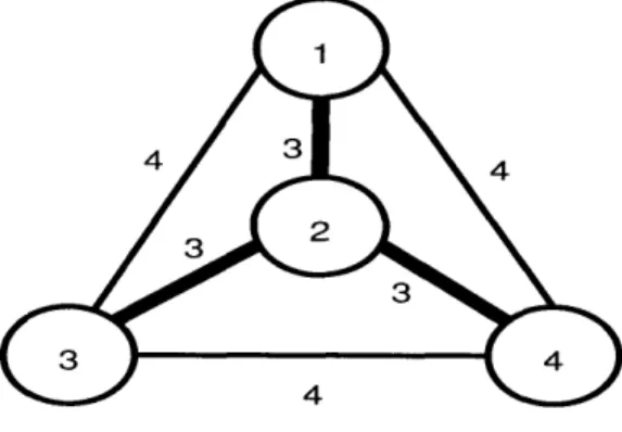
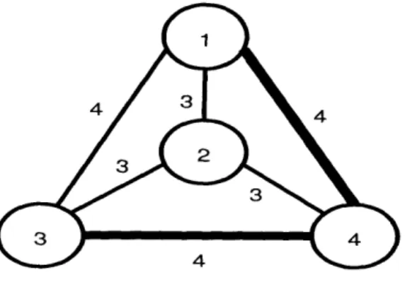
As it was discussed in chapter 1, the aim of the sensor which receives the query is to form a tree that spans the nodes that participate in the aggregate and has the lowest possible cost in some metric that affects its operation. The cost of a tree is defined to be the sum of the costs of the edges that it is comprised of. This is known as the Minimum Steiner Tree problem in graph theory. Generally, a Steiner tree is a tree that spans a set of required nodes. A spanning tree is also a Steiner tree but the minimum Steiner tree is not always the same as the minimum spanning tree. For example, consider the minimum spanning tree of the graph in figure 2.1. The minimum Steiner tree that spans nodes 1, 3 and 4 is shown in figure 2.2 and it is not a subset of the minimum spanning tree.
Figure 2.1: Minimum Spanning Tree
The computation of the Minimum Steiner Tree requires the consumption of a large amount of com-munication or energy resources, as proven in [7]. The aim is to construct a tree with low cost that is not expensive to create. It is clear that there is going to be a trade-off between the cost of the Steiner tree and the resources spent for its formation. The goal is to construct a protocol that will consume a reasonable amount of resources and at the same time form a tree which computes aggregates without large energy consumption. Of course, the frequency of using the aggregation tree should be considered.
CHAPTER 2. BACKGROUND
4
4
4
Figure 2.2: Minimum Steiner Tree
If it is used very frequently or for many times, it is worth spending more resources in order to construct it.
The Minimum Steiner Tree problem is an NP-hard problem even in its centralized version [7, 15]. The nodes that need to be spanned are called required nodes and any additional ones required to form the tree are called steiner nodes. Let n be the number of required nodes and s be the number of steiner nodes. There exists an algorithm which computes the Minimum Steiner Tree in O(n22s) time,
namely polynomial in n [13]. The Dreyfus-Wagner algorithm computes the Minimum Steiner Tree in
O((n + s)3n + (n + s)22n) time, which is polynomial in n + s [13].
Since we would like to spend a small amount of computation and communication resources to con-struct the region, we are going to consider approximation algorithms that compute a suboptimal Steiner Tree. There is an approximation algorithm for the centralized version of the Steiner tree problem that
achieves a factor of 2 approximation [7].
2.4.1 The metric Steiner tree problem
There is a specific version of the problem, which is called the metric Steiner Tree problem. The metric Steiner Tree problem is the Steiner problem for a graph G(V, E), which is complete and satisfies the triangle inequality, namely for every triplet of nodes (a, b, c), cost(a, c) < cost(a, b) + cost(b, c). It can be proved that any approximation factor achieved for the metric Steiner problem can be carried over to the general Steiner Tree problem [7].
Let G(V, E) be the graph for which we would like to solve the general Steiner Tree problem. Let G'
2.5. BUILDING A NEW PROTOCOL
be the complete graph on the set of vertices V, such that the cost of every edge (a, b) is the cost of the shortest path from a to b in G. Let T' be a Steiner tree in G'. Then, we can construct a Steiner tree
T in G that has cost at most equal to the cost of T'. For every edge in T', we find the corresponding
shortest path in G and add its edges in T. The resulting graph may contain cycles. We remove those cycles to get T. Thus, the cost of T is at most equal to the cost of T'.
Let G be a complete graph that satisfies the triangle inequality. Let R be a set of required vertices. There is an approximation algorithm which solves the Steiner tree problem with a factor of 2. This algorithm computes the minimum spanning tree for the subgraph of G that contains only R and the edges of G that connect 2 vertices in R. Let Tapp be this tree. Let Topt be the optimal Steiner tree
over R in G. Topt does not contain any Steiner vertices because if it contained a path (Pl,P2,... ,Pk),
where P1 and Pk are required vertices and all P2,P3,... ,Pk-1 are Steiner vertices, then this path could be replaced with the edge (Pl,Pk), which would have cost less than or equal to the cost of the whole path, due to the triangle inequality. Let OPT be the cost of Topt.
We consider ea cycle in graph G, which starts from the root of the tree Topt, visits all the nodes of it
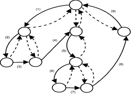
in a depth-first order and returns to the root. Each edge of the tree is traversed twice and thus, the total cost of the cycle is twice the cost of the tree, which is OPT. An Euler tour is a path which uses each edge exactly once. If the traversed edges were double, then this would be an Euler tour, because each
edge would be traversed only once (figure 2.3). A Hamiltonian cycle is a cycle which visits each node
of the graph exactly once. We can obtain a Hamiltonian cycle that starts from the root and returns to the root by following the Euler tour and every time the Euler tour revisits some node following the edge which leads directly to the next in the order node (figure 2.4). The direct edge has cost less than or equal to the cost of the edges in the Euler tour. That is why the Hamiltonian cycle has cost less than
or equal to 2 OPT. If we remove an edge from the Hamiltonian cycle, we get a spanning tree that has
cost less than or equal to 2 OPT. So, the optimal spanning tree Tapp has cost at most equal to 2 OPT too.
2.5 Building a new protocol
The ideas, the principles and the algorithms used in the Regions project, Tiny AGgregation (TAG), the probabilistic query model and the Steiner Tree theory can be used to define a protocol that constructs aggregate trees such that aggregate values are calculated spending less energy and time. We should
CHAPTER 2. BACKGROUND (1) (16) (2) (13) (9) (12)
Figure 2.3: Depth first Euler tour traversal of the Minimum Spanning Tree
Figure 2.4: Depth first Hamiltonian path traversal of the Minimum Spanning Tree
2.5. BUILDING A NEW PROTOCOL 25
identify metrics or the wireless links that affect the consumed energy while computing aggregates, as well as the time spent to propagate the partial state records to the root. Once the metrics are defined,
Chapter 3
Classifying functions
It is useful to classify functions according to their capability of being divided into multiple segments. In this case, the segments of the function can be calculated in different sites in a sensor network. If the values that each segment returns have small representation sizes, they can be transmitted to a central computation point and avoid sending all the parameters of the initial function.
3.1
Functions that can be divided into segments
Each segment of a function division is also described by a function. The segmentation of a function consists of the set of functions that should be calculated for the computation of the returned value of the segmented function, the arguments over which they are going to be applied and the function that will return the final result.
Let us consider a function f that takes n arguments al, a2, ... , an. Each one of the arguments is a
piece of data. We assume that function s returns the size of the representation of a piece of data. The expression s(ai), I < i < n denotes the size of the representation of the argument ai.
In a distributed computation environment, the size of the intermediate results, which are the re-turned values of the segmentation functions, determines the total amount of information that should be communicated in order to produce the returned value of the segmented function. A division of functions into classes according to segmentation capability should take into consideration this property. The use of a segmentation. in order to compute a function should reduce the total amount of information that
CHAPTER 3. CLASSIFYING FUNCTIONS
needs to be transmitted compared to the case when no segmentation is applied.
3.1.1
Partitionable or decomposed functions
We can provide a definition for partitionable or decomposed functions, taking these facts into consider-ation. A function f with arguments al, a2, ... , an is called partitionable or decomposed if there exists
a partition of the set a = {al, a2,..., an} into disjoint sets gl, g2, .., gm and there exist functions fc,
fl .. , fi, such that for every possible vector of values assigned to (al, a2, ..., an),
f(al, a
2,...,an) = fc(fl(gl),f
2(g
2),..., fm(gm))
andVi
{1,2,...,m}
s(fi(gi)) < E s(aj).jCI(gi)
I(gi), i (1, 2,..., m}, is the set of the indexes of the arguments aj that are members of gi.
Average is a partitionable function. Let AVERAGE(a, a2,...,an) denote the average of numbers
a, a2, ..., an. Then,
AVERAGE(a,
a
2,
...
,an) - iLet us consider the partition g = {al,a2,...,a ]}, g2 = {a[nl+l,a[l+ 2 .. an}. If fp(al, a2,
an) (En ai, n)
and f((al,,
al,2), (a2,,
a2,2)): a',+a2,1then f(al,a
2, ... ,an) f(fp(a
a2, ... , ar[1), fp(a[rl+ 1, a[i1+2 .. ., an)). The representation of each number takes a certain number
of bits. f takes as arguments n numbers, whereas f takes as arguments 2 couples of numbers. For
n > 4, the sum of the sizes of the returned values for the intermediate results is smaller than the sum of
the sizes of the arguments of AVERAGE. Those observations imply that AVERAGE is a partitionable function.
In the same way, we can prove that functions max and min are partitionable. Observe that max(a1, a2, ... , an) = max(max(al, a2, ... , am), max(am+i, am+2, ... , an)) for every m such that 1 < m < n-.
The same segmentation can be applied to the min function.
3.1.2 Monolithic functions
If a function is not partitionable or decomposed, it is called monolithic. In order to provide the definition for monilithic functions, we have to define a matching function set for a partition of a set of data a =
3.1. FUNCTIONS THAT CAN BE DIVIDED INTO SEGMENTS
{al, a2,.. , an} into disjoint sets gl, g2, ... , g. A set of functions f =
{fc,
fl, f2, . ., fn} is a matching function set for a partition of a set of data a = {al,a2, ... ,an} into disjoint sets gl, g2, .. , gi, if forevery i {1,2,...,n}, gi belongs to the domain space of fi, and (fl(gl),f 2(g2), ., fm(gm)) belongs
to the domain space of ft. In other words, each fi, < i < n can be applied to gi and fc can be applied
to the vector with the returned values of all functions fi, 1 < i < n.
The definition of monolithic functions is generated by negating the definition of partitionable func-tions. A function f with arguments al, a2, ..., a, is called monolithic if for all possible partitions
of the set a = al,a 2,...,an} into disjoint sets gl, 92, , gm and for all matching function sets
(fc, f, f2,.. , f,,), there exists an assignment t = (t t, t,..., tn) to the vector (al, a ..
2 ., an), such that
f(t
1
,t
2
. .
,
.
,t)
fc(fl(gl(t)),f
2
(g
2
(t)),.. fm(gm(t))
or
3i C {1,2,...,m} such that s(fi(gi)) > s(aj).
jEl(gl)
gi(t), 1 < i < m, denotes the subset of the assignment t that corresponds to group gi of the partition.
An example of a monolithic function is the one which returns the JOIN of two tables. If we divide the entries of the two tables into groups, we can compute the JOIN of all those parts and then, combine the results. If two parts contain x and y entries respectively, then, their JOIN will contain x · y entries. So, the total size of the partial results is going to be larger than the size of the two initial tables. That is why the JOIN function is monolithic.
3.1.3
Fully partitionable functions
Some partitionable functions have the extra property that their computation can be divided into groups for every possible partition of their arguments. Such a property provides additional flexibility when trying to assign computation tasks in a distributed environment. The partitionable functions that hold this property are called fully partitionable. A function f with arguments al, a2, ... , an is called fully partitionable if for all partitions of the set a = {al, a2,..., an} into disjoint sets gl, g2, ... , g, there exist functions f. fl ... , fin, such that for every possible vector of values assigned to (al, a2., an),
f(al, a2,..., an) = f(fl(gl), f2(g2) , fm(gm))
and
CHAPTER 3. CLASSIFYING FUNCTIONS
Vi {1,2,..., m} s(fi(gi)) < E s(aj).
jEI(gi)
Let us consider the function AVERAGE. This is proved to be fully partitionable. Consider a partition
gl, g2, ..., gm of its arguments into disjoint sets. Then,
AVERAGE(ai, a2,... ,an)
3
[giAVERAGE(gi) i-1The size of each Ig-iAVERAGE(gi) is equal to the size of a number. So, the size of all the returning
values of the intermediate functions is equal to m times the size of a number. The initial parameters have total size equal n times the size of a number and m < n. Thus, AVERAGE is a fully partitionable function. In the same way, max and min are proved to be fully partitionable.
3.1.4
Recursive functions
There are some functions that can take any number of arguments. They treat each argument in the same way. This means that for every possible ordering of the arguments, the returned value remains the same. It is interesting to check if such functions are partitionable. In the case that they are partitionable, it is important to see if the functions that consist the segments of their computation are the same as the segmented function. Functions that hold this property are called recursive.
A function f with arguments al, a2, ... , an is called recursive if for all possible partitions of the set a = {al, a2,..., an} into disjoint sets gl, g2, ... , gm and for every possible vector of values assigned
to (al,a2,...,an),
f(al, a2,
..
, an)
= f((g), f(g
2),
f(gm))
This definition states that we may divide the set of arguments into disjoint sets in any way, apply the function to each one of them and then, apply the function to the returned values of those partial results in order to get the final result. This is very important in a distributed computation environment because it provides flexibility in the computation plan.
Let us consider the function max. This is proved to be recursive. Consider a partition gl, g2,.., gm of its arguments into disjoint sets. Then,
max(al, a2,..., an) = max(max(gl), max(g2),..., max(gm))
The size of max(gi), 1 < i < m, is the representation size of a number. So, the total size of the returned values of the intermediate functions is m times the representation size of a number. The
3.2. AGGREGATE FUNCTIONS
arguments of the initial functions have total size equal to n times the representation size of a number. Since, m < n, we have that max is a recursive function. In the same way, function sum is proved to be recursive.
3.2 Aggregate functions
Aggregate functions are special functions that provide us with extensive flexibility when trying to divide them. Each aggregate function has the following properties:
1. It can be applied to any number n of arguments, n > 1.
2. It treats all arguments in the same way. This means that AGGREGATE (x) = AGGREGATE
(p(x)), for every permutation and every vector of values x.
Examples of aggregate functions are AVERAGE, COUNT, MAX, MIN, SUM, VARIANCE and HISTOGRAM. In [3], the method of computing aggregate functions by partial state records is proposed. The size of the partial state records affects the category of the aggregate functions. The partial state records are the results of the intermediate functions. In distributive aggregates, the partial state record is identical to the aggregate over the partition it represents. Thus, distributive aggregates are recursive functions. In algebraic aggregates, the partial state records have constant size. Consequently, they are
fully partitionable functions.
3.3 The importance of decomposing functions
As it was discussed, it is very important to decompose the computation of a function into segments. The production of intermediate results requires the communication of smaller amounts of information and if their size is also small, the final result will be computed without spending too much communication resources.
The partitionable, monolithic, fully partitionable or recursive functions form classes of functions declaring interesting properties about the segmentation of their computation. Aggregate functions present useful properties regarding their segmentation. The fact that algebraic aggregates are fully partitionable functions and distributive aggregates are recursive functions makes the attempt to con-struct protocols that compute aggregates in sensor networks using those properties challenging.
Chapter 4
Resource Management in Sensor
Networks
Progress that has been made in the field of computing devices has led to the construction of wireless, battery powered, smart sensors. The sensors are able to measure attributes of their environment, observe phenomena that take place near their location, combine data and produce filtered information. An example of such small sensor devices are the motes which were developed at UC Berkeley [24].
The motes are small devices that have dimensions 2 cm x 4 cm x 1 cm and they contain a pro-cessor, a memory, a small battery pack, and a set of sensing devices. They run a special operating system designed or them, the TinyOS. TinyOS provides an environment that allows modularity and a resource-constrained, event-driven concurrency model, which is valuable because of the large number of information flows that each sensor processes [24].
The limited resources of sensors make use of resource management techniques vital in the operation of sensor networks. The computation power and the energy that every sensor has should be used in an optimized way that increases the lifetime of sensors and, through this, the amount of useful information that we get from the network.
Regarding data, we consider two cases. In the first case, the application which submits the query prefers to have all pieces of data but is willing to operate even it does not have them. In the second case, the sensors do not want to have all pieces of data. In any case, we try to combine the application's
CHAPTER 4. RESOURCE MANAGEMENT IN SENSOR NETWORKS
needs with the energy and communication resources.
4.1 The case of aggregate queries
Aggregate queries are very common in sensor networks. Very often, we deploy a set of sensors in an environment and we would like to receive one value that represents all the values that the sensors measured. In this case, we are not interested in having every single piece of raw information but the result of a function applied to them. It is clear that the result has much smaller size than the initial information. That is why we would like to have the network produce the result and then, forward it to the user of this information.
4.1.1
Considering TAG performance
Tiny AGgregation (TAG) [3] is a paradigm for achieving resource management in sensor networks that compute aggregate queries. It constructs a tree that spans all the nodes in the network and produces the aggregate value without having all the nodes send the measured value to the computation point.
TAG computes a spanning tree randomly. The total number of transmissions is not taken into consideration and all the links are considered to have the same quality. The question of whether there are some spanning trees that achieve better performance in terms of the consumed energy arises.
In some cases, we do not need to compute the aggregate over all the sensors in the network but over some subset of them. TAG provides us with a way to do this. We have to insert predicates in the WHERE or the HAVING part of the SQL query. Those predicates will make sure that the values which will be propagated up towards the root of the tree will be the ones that satisfy the predicates mentioned in the query.
As we observe, the same tree that spans all the network is used even if we would like to gather information from some small subset of the nodes. The communication overhead because of using the whole network tree increases when the subset of nodes is located in a part of the network. Most of the transmissions that will be made are going to be useless. If we had a smaller tree, we could compute the aggregate making a much smaller number of transmissions and much quicker.
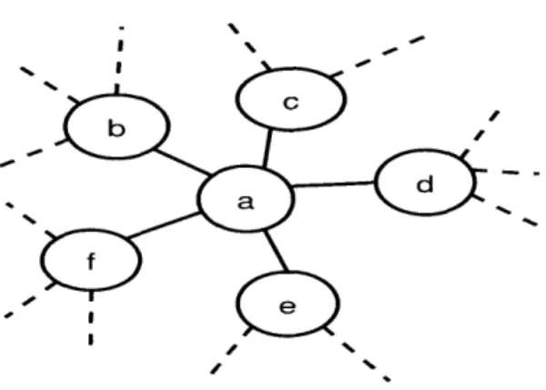
Consider the case of the network in figure 4.1. Most of the transmissions that will happen are useless. We could have a tree that consists of the root node and its 1-hop neighbors that would do the
4.1. THE CASE, OF AGGREGATE QUERIES
computations spending much less resources. %
Figure 4.1: Computing aggregate for some part of the network
Also, some links have better quality than others. In a congested link, the number of trials to submit successfully will be large. So, the total energy that will be lost for tranmission across this link will be high. For this reason we should choose high quality links when making the aggregation tree.
4.1.2 Optimizing the aggregation tree
The first observation that we make while trying to optimize the aggregation tree is that in many cases the aggregation that should be carried out does not refer to the whole network but only to some subset of its nodes. This is very important when we have a network consisting of a large number of nodes and we want it to address scalability.
Given that there does not exist routing information for any node in the network and that we want to guarantee that all participating nodes will be found, we expect that we should search the network in all directions until we find the nodes that participate in the aggregate. This is what TAG does. But even if we search all the network to find the nodes that we want to participate in the query, we do not have to maintain the tree that spans the whole network. We can just maintain the portion of it that spans the query nodes. In this way, the total energy and time spent to compute an aggregate will go down. This will produce increased savings as the tree is used repeatedly.
Moreover, if we find all the query nodes in the searching process, we can stop it and avoid flooding all the network. To achieve this, we should have a mechanism that identifies when this is done and informs all searching processes to stop. This is quite difficult when there are a lot of searching processes.
35
I I
CHAPTER 4. RESOURCE MANAGEMENT IN SENSOR NETWORKS
Another matter that arises while trying to construct the tree is the quality of the links that comprise it. We assume a metric that measures the link quality and has the property that the quality of a path is the sum of the qualities of its links. In this case, the construction of the tree gets even more complicated. Even if we find a node, we are not sure which is the optimal way to connect it to the aggregation tree. Even in the simplest case, when the metric of every link is equal to 1 and we aim to minimize the number of hops, it is difficult to find the optimal routes.
The choice of the link quality metric depends on the operation parameter that we want to optimize. We assume the method for computing aggregates that is proposed by TAG. Each node receives the partial state aggregation records from its children and merges them to produce the partial state record that represents all the records that it received from its children. If it also participates in the aggregate, it merges those records with its own record too.
Energy constraints are very important in sensor networks. That is why we would like to use a metric such that the total cost of the tree is proportional to the total energy spent to compute an aggregate value. It is also important to compute aggregate values in a small amount of time. In this case, we have to use a metric that is proportional to the total amount of time needed to produce an aggregate value at the root of the tree. Sometimes, we might want to take into consideration both parameters. In those case, we will use a linear combination of the 2 metrics with weights determining the importance of each parameter in our scheme.
4.2 Minimizing energy
As sensors are battery operated, they have limited energy. That is why we would like to compute the aggregate values using the minimum possible energy. The energy consumed by a sensor device is used for sensing, computing and communicating information. To minimize the total energy consumption we should take into consideration the amount of energy spent for each aim.
The energy spent in sensing depends on the kind of phenomena or attributes that we would like to sense, as well as the sensing sampling frequency. If the aim to minimize the total energy spent to compute a single aggregation value is considered, the sensing energy spent is proportional to the number of sensors participating in the aggregate. Of course, in the case that a probability distribution for the request pattern is considered, the sampling frequency is affected, which needs to be examined for the computation of the total energy consumed. The energy spent for sensing is, generally, small compared
4.2. MINIMIZING ENERGY
to the one spent for communication.
The computation energy is the energy spent to carry out the mergings. This depends on the kind of aggregate that is computed, which determines the size of the partial state records. It is also influenced by the hardware and the computing architecture. In [25], Levis et al. propose the use of application specific virtual machines to reprogram sensor networks, in order to achieve energy efficiency. As in the case of sensing energy, this amount of energy is also small compared to the one used for communication. The communication energy refers to the cost of communicating the partial state records, as well as the energy spent while waiting to receive them. The transmission energy is also affected by the size of the records and thus, by the kind of aggregate that is computed. If we assume that the energy spent for every transmission is the same, the total transmission energy cost is proportional to the number of edges in the spanning tree.
The assumption that the transmission energy cost across all links will be the same is not always accurate, though. The transmissions are accomplished using some MAC protocol. Every shared media protocol is going to have some overhead that consumes energy. If the overhead is large, the transmission energy spent to communicate a partial state record through a link is going to be high. This overhead is affected by the congestion in the area in which the transmission will occur. If many sensors try to transmit informaltion, then a large number of collisions will occur and the total energy spent for successful transmission will be high. The metric that will be chosen for the links should be proportional to the average amount of energy spent to transmit successfully a partial state record.
In TAG, the energy spent while waiting to receive information is small compared to the one used for transmitting information. This is true because each epoch is divided into time intervals and each sensor needs to receive information for only one time interval per epoch. The length of this time interval is proportional to _, where TE is the duration of the epoch and d is the depth of the aggregation tree. Thus, the fraction of time that a sensor needs to be awake in order to receive the partial state records is small and the energy spent for it is small compared to the energy spent for transmissions.
4.2.1 Analyzing the tranmission control mechanism
The media used to propagate information in a wireless network is the air. This is a shared media, which makes the use of a media access control protocol necessary. When a sensor sends some signal, all the other sensors that are within its range can hear it. Therefore, they cannot receive another signal at the