MIT Joint Program on the
Science and Policy of Global Change
The Cost of Kyoto Protocol Targets:
The Case of Japan
Sergey Paltsev, John M. Reilly, Henry D. Jacoby and Kok Hoh Tay
Report No. 112
The MIT Joint Program on the Science and Policy of Global Change is an organization for research, independent policy analysis, and public education in global environmental change. It seeks to provide leadership in understanding scientific, economic, and ecological aspects of this difficult issue, and combining them into policy assessments that serve the needs of ongoing national and international discussions. To this end, the Program brings together an interdisciplinary group from two established research centers at MIT: the Center for Global Change Science (CGCS) and the Center for Energy and Environmental Policy Research (CEEPR). These two centers bridge many key areas of the needed intellectual work, and additional essential areas are covered by other MIT departments, by collaboration with the Ecosystems Center of the Marine Biology Laboratory (MBL) at Woods Hole, and by short- and long-term visitors to the Program. The Program involves sponsorship and active participation by industry, government, and non-profit organizations.
To inform processes of policy development and implementation, climate change research needs to focus on improving the prediction of those variables that are most relevant to economic, social, and environmental effects. In turn, the greenhouse gas and atmospheric aerosol assumptions underlying climate analysis need to be related to the economic, technological, and political forces that drive emissions, and to the results of international agreements and mitigation. Further, assessments of possible societal and ecosystem impacts, and analysis of mitigation strategies, need to be based on realistic evaluation of the uncertainties of climate science.
This report is one of a series intended to communicate research results and improve public understanding of climate issues, thereby contributing to informed debate about the climate issue, the uncertainties, and the economic and social implications of policy alternatives. Titles in the Report Series to date are listed on the inside back cover.
Henry D. Jacoby and Ronald G. Prinn,
Program Co-Directors
For more information, please contact the Joint Program Office
Postal Address: Joint Program on the Science and Policy of Global Change
77 Massachusetts Avenue MIT E40-428
Cambridge MA 02139-4307 (USA)
Location: One Amherst Street, Cambridge
Building E40, Room 428
Massachusetts Institute of Technology
Access: Phone: (617) 253-7492
Fax: (617) 253-9845
E-mail: g l o ba l ch a n g e @ m i t .e d u
Web site: h t t p:/ / M I T .E D U / g l o ba l ch a n g e /
The Cost of Kyoto Protocol Targets: The Case of Japan
Sergey Paltsev, John M. Reilly, Henry D. Jacoby and Kok Hou Tay Abstract
This paper applies the MIT Emissions Prediction and Policy Analysis (EPPA) model to analysis of the cost of the Kyoto Protocol targets, with a special focus on Japan. The analysis demonstrates the implications of the use of different measures of cost, and explains the apparent paradox that the relative carbon price among Kyoto parties may not be an accurate measure of their relative welfare costs. Attention is given to the role of relative emissions intensity and various distortions, in the form of fuel and other taxes, in determining the burden of a climate policy. Also, effects of climate policy on welfare through an influence on the terms of trade are explored. We consider the cases of the EU, Japan, and Canada, each meeting their Kyoto targets, and the US meeting the Bush Administration’s intensity target. For a country with a low emissions intensity as in Japan, the absolute reduction in tons is small relative to the macroeconomy, and this reduces its welfare loss as a share of total national welfare. Low emissions intensity (high energy efficiency) also means the economy has few options to reduce emissions still further, resulting in a higher carbon price. Energy efficiency thus pushes in both directions, lowering the number tons that need to be reduced but raising the direct cost per ton. But other factors also are important in explaining costs differences. Existing fuel taxes are very high in Japan and Europe, increasing the economic cost of a greenhouse gas emissions reduction policy. For these regions, the extra cost due to these distortions is several times the direct cost of the emissions mitigation policy itself. In contrast, fuels taxes are low in the US and relatively low in Canada. The US, EU, and Japan gain somewhat from reductions in world prices of oil and other fuels because they are net importers. Canada, in contrast, is a significant net energy exporter, and its policy costs rise considerably because of lost energy export revenue. This effect on Canada is due mostly to implementation of the policy in the other regions rather than to domestic implementation. Canada is also the most emissions intensive of these regions, a factor that contributes to its cost of control.
Contents
1. Introduction ... 1
2. The EPPA Model ... 4
3. Implementation Options for Japan ... 6
3.1 Cases Studied ... 6
3.2 Simulation Results ... 8
4. Cost Concepts and Why Countries Differ... 10
4.1 An Equal-Reduction Comparison... 10
4.2 The Influences on National Cost ... 12
5. Decomposition of Costs: Numerical Analysis ... 20
5.1 Analysis Method ... 20 5.2 Necessary Approximations... 21 5.3 Numerical Results ... 23 6. Conclusions ... 24 7. References ... 26 1. INTRODUCTION
There have been many studies of the cost to Annex B countries of meeting Kyoto Protocol commitments. Unfortunately for these analyses, the Protocol has proved to be a moving target in terms of its interpretation and likely implementation. In addition, the economic performance and future expectations for some parties also are changing, and with these changes come revisions in
reference emissions, which have a strong influence on the projected cost of meeting Protocol requirements. Looking back across these studies, the progression of work can be divided into three broad phases. The first studies were conducted soon after the Protocol was signed in 1997, and they focused on carbon emissions from fossil fuels. Often they assumed idealized system of harmonized carbon taxes, or cap-and-trade among all the Annex B parties, contrasting such systems with implementation without international permit trade but with an idealized trading system operating within each country (see, for example, Weyant and Hill, 1999). These studies showed a high cost of the Protocol with autarkic compliance, but huge benefits of international trading because it made Russian hot air accessible to other Annex B parties.
A second phase of studies followed the final negotiations in Marrakesh in 2001 (Bohringer, 2001; Babiker et al., 2002; Manne and Richels, 2001). By that time, the US had withdrawn from the Protocol, and the potential contribution of Article 3.4 carbon sinks had been defined for each Party. Progress in economic modeling also made it possible to consider the economic cost and contribution of non-CO2 greenhouse gases. These changes—US withdrawal, added sinks, and the
consideration of non-CO2 GHGs—led to downward revisions in the cost of meeting the Protocol,
particularly if idealized trading among the remaining Annex B parties was assumed (Babiker et al., 2002). In fact, many analyses concluded that credits from Russian hot air, and to lesser extent from Eastern European Associates of the EU, could be sufficient to meet Kyoto targets without additional effort.
We are now in a third phase of this work, where studies seek to estimate the cost under a more realistic representation of how the target reductions might actually be achieved. These studies seek to understand the cost of a mixed set of policies that almost certainly will differ among Kyoto parties and across economic sectors, and that will thus be more costly than the idealized systems studied earlier. Some elements of such “imperfect” implementation have been
considered in past studies. Examples include the potential for the exercise of monopoly or monopsony power in the permit market (e.g., Ellerman and Sue Wing, 2000; Bernard et al., 2003), the impact of pre-existing tax distortions on labor and capital (e.g., Shackleton et al., 1993; Goulder, 1995; Fullerton and Metcalf, 2001) or on energy (Babiker et al., 2000c), and policies focused on particular technologies or sectors (e.g., Babiker et al., 2000a; Babiker et al., 2003a). In this analysis we extend and interpret this work.
To realistically study these latter aspects of cost requires attention to the exact set of policies and measures likely to be implemented, and representation of ways they will interact with existing tax policies. Because circumstances can differ among countries and across sectors, a result that holds in one country may not hold in another. For example, much analysis of the double-dividend (from the use of carbon revenue to reduce distorting capital and labor taxes) has been conducted in the United States, and these studies have found evidence of at least a weak double-dividend. But recent work has shown a much smaller double-dividend effect in other Annex B countries (Babiker et al., 2003b). This result occurs because reducing labor taxes
within a particular fiscal structure may further distort relative prices by widening the divergence between labor rates and energy prices (tax inclusive). Where this happens, the distorting effect may offset other potential gains of revenue recycling.
Furthermore, the presence of varying distortions and fragmented policy implementation across countries raises questions about the degree to which a party can take advantage of the various international flexibility mechanisms, and, if they do, whether such trading is in fact welfare enhancing. Without comparable trading systems that can be linked, and absent the willingness of parties to permit unrestricted cross-border trading, international flexibility may exist only on paper. Recent studies emphasize that extreme care is needed in the design of policies to make them economically efficient, and they highlight the difficulty of realistically achieving the low costs found under idealized cap-and-trade systems. Thus, the Protocol could end up being relatively costly for some parties but, without the US involved, it will not achieve nearly the environmental benefit imagined when it was signed in Kyoto. While international emissions trading has been shown to be beneficial for all parties when trading includes the hot air from Russia and Eastern European Associate nations, this result has not held up in more limited trading scenarios. In these cases trading may not be beneficial to all parties, even if they enter into the system voluntarily—a result that can be traced to the interaction of the carbon policy with existing energy taxes (Babiker et al., 2004).
The conclusion that the Protocol may entail relatively high cost with limited environment benefit thus stems from consideration of three factors: (1) domestically it appears almost certain that no Kyoto party will implement an economy-wide tax or cap-and-trade system covering all of its emissions of all greenhouse gases, and the Protocol allows only limited the use of
economically attractive forest and agricultural sinks; (2) the international flexibility mechanisms will almost certainly not work in the ideal manner represented in many economic models; and (3) policies implemented by parties may interact with existing taxes and economic distortions in a way that raises the cost of those measures.
As the set of issues addressed by these economic modeling studies has become richer and more complex, the definition of economic cost itself, and how it is estimated in economic
models, has presented a puzzle, particularly to those outside the economic modeling community. Depending on the study, cost results may be reported in various ways, e.g., in terms of the carbon or carbon-equivalent price of GHGs, as the integrated area under an abatement curve, or
applying broader measures of economy-wide welfare such as the reduction in consumption or GDP. Adding to the confusion thus created is the fact that the costs of a policy as estimated by different concepts, even using a single model, often appear inconsistent. For example, early studies examining Kyoto costs without international emissions trading showed Japan to have the highest carbon price, followed by the US and other OECD regions, and the EU. But, among this group the cost in percentage loss of welfare was lower in Japan than in the EU. The apparent
inconsistency of these results, where the ranking of cost by one measure is reversed when another is used, emphasizes the importance of distinguishing among these cost concepts.
In this paper we explore these concepts and the differences among them. By focusing on Japan we are able to consider in some detail the implication of alternative domestic
implementation strategies. Of course, understanding the costs to Japan, with or without the international flexibility mechanisms provided in the Protocol, necessarily requires specification of the policies followed by other parties. The results reported here are in the domain of the third phase of studies outlined above, where more complex and more realistic policies (not necessarily designed for economic efficiency) are the focus of analysis. To be sure, Kyoto’s entry into force is still very much in doubt, with the domestic policy details of most parties still not specified, so possible costs to Japan or any other Party remain speculative. Nevertheless, this work can pave the way toward a likely fourth phase of studies, where it will be necessary to investigate the costs and effectiveness of policies actually implemented—whether intended to achieve the Kyoto targets or other goals.
We begin the analysis with an overview of the EPPA model used to perform the simulations. In Section 3 we lay out a set of policies designed to study possible implementation of the Kyoto Protocol in Japan and elsewhere and compare these costs across countries and regions using two of the more common measures of cost. Section 4 addresses the question of why different costs concepts produce paradoxical results about the cost of Kyoto in Japan compared to other countries, and explores the various factors that contribute to the welfare cost in any country. In Section 6 we provide a numerical decomposition of the consumption loss, showing how the various components sum to the overall welfare cost in each of the four regions studied. Finally, Section 7 offers some conclusions.
2. THE EPPA MODEL
The EPPA model is a recursive-dynamic multi-regional general equilibrium model of the world economy, which is built on the GTAP dataset (Hertel, 1997) and additional data for greenhouse gas (CO2, CH4, N2O, HFCs, PFCs and SF6) and urban gas emissions (Mayer et al.,
2000). The version of EPPA used here (EPPA 4) has been updated in a number of ways from the model described in Babiker et al. (2001). Most of the updates are presented in Paltsev et al. (2003). The various versions of the EPPA model have been used in a wide variety of policy applications (e.g., Jacoby et al., 1997; Jacoby and Sue Wing, 1999; Reilly et al., 1999; Paltsev et al., 2003). Compared with the previous EPPA version, EPPA 4 includes (1) greater regional and sectoral disaggregation; (2) the addition of new advanced technology options; (3) updating of the base data to the GTAP 5 data set (Dimaranan and McDougall, 2002) including newly updated input-output tables for Japan, the US, and the EU countries and rebasing of the data to 1997; and (4) a general revision of projected economic growth and inventories of non-CO2 greenhouse
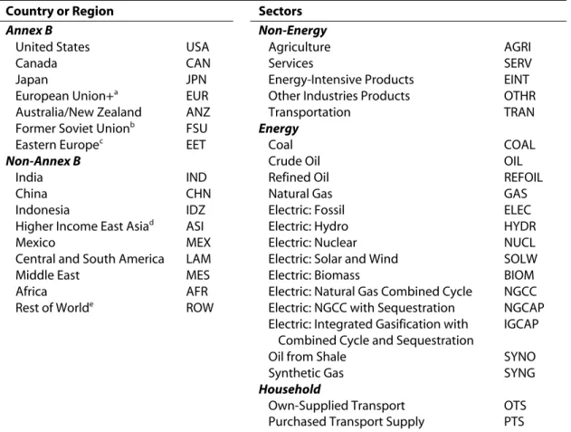
EPPA 4 aggregates the GTAP dataset into 16 regions and 10 sectors shown in Table 1. The base year for the EPPA 4 model is 1997. From 2000 onward, it is solved recursively at 5-year intervals. To better focus on climate policy, the model is disaggregated beyond than provided in the GTAP data set for energy supply technologies and for transportation, and a number of supply technologies are included that were not in use in 1997 but could take market share in the future under some energy price or climate policy conditions. All production sectors and final
consumption are modeled using nested Constant Elasticity of Substitution (CES) production functions (or Cobb-Douglas and Leontief forms, which are special cases of the CES). The model is written in the GAMS software system and solved using the MPSGE modeling language.
The regional disaggregation of EPPA 4 includes a breakout of Canada from Australia/New Zealand, and a breakout of Mexico to better focus on North America. Developing country regional groupings were altered to create groups that were geographically contiguous. Table 1. Dimensions of the EPPA Model
Country or Region Sectors
Annex B Non-Energy
United States USA Agriculture AGRI
Canada CAN Services SERV
Japan JPN Energy-Intensive Products EINT
European Union+a EUR Other Industries Products OTHR
Australia/New Zealand ANZ Transportation TRAN
Former Soviet Unionb FSU Energy
Eastern Europec EET Coal COAL
Non-Annex B Crude Oil OIL
India IND Refined Oil REFOIL
China CHN Natural Gas GAS
Indonesia IDZ Electric: Fossil ELEC
Higher Income East Asiad ASI Electric: Hydro HYDR
Mexico MEX Electric: Nuclear NUCL
Central and South America LAM Electric: Solar and Wind SOLW
Middle East MES Electric: Biomass BIOM
Africa AFR Electric: Natural Gas Combined Cycle NGCC Rest of Worlde ROW Electric: NGCC with Sequestration NGCAP
Electric: Integrated Gasification with Combined Cycle and Sequestration
IGCAP
Oil from Shale SYNO
Synthetic Gas SYNG
Household
Own-Supplied Transport OTS Purchased Transport Supply PTS
a
The European Union (EU-15) plus countries of the European Free Trade Area (Norway, Switzerland, Iceland).
b
Russia and Ukraine, Latvia, Lithuania and Estonia (which are included in Annex B) and Azerbaijan, Armenia, Belarus, Georgia, Kyrgyzstan, Kazakhstan, Moldova, Tajikistan, Turkmenistan, and Uzbekistan (which are not). The total carbon-equivalent emissions of these excluded regions were about 20% of those of the FSU in 1995. At COP-7 Kazakhstan, which makes up 5-10% of the FSU total, joined Annex I and indicated its intention to assume an Annex B target.
c
Hungary, Poland, Bulgaria, Czech Republic, Romania, Slovakia, Slovenia.
d
South Korea, Malaysia, Phillipines, Singapore, Taiwan, Thailand.
e
New sectoral disaggregation includes a breakout of services (SERV) and transportation (TRAN) sectors. These were previously aggregated with other industries (OTHR). This further
disaggregation allows a more careful study of the potential growth of these sectors over time, and the implications for an economy’s energy intensity. In addition, the sub-model of final
consumption was restructured to include a household transportation sector. This household activity provides transportation services for the household, either by purchasing them from TRAN or by producing them with purchases of vehicles from OTHR, fuel from ROIL, and insurance, repairs, financing, parking, and other inputs from SERV. While the necessary data disaggregation for TRAN is included in GTAP 5 (Dimaranan and McDougall, 2002), the creation of a household transportation sector required augmentation of the GTAP data as described in Paltsev et al. (2004).
3. IMPLEMENTATION OPTIONS FOR JAPAN 3.1 Cases Studied
In order to study the potential cost of the Kyoto Protocol to Japan, a number of assumptions are required. The Protocol has not yet entered into force, and exactly how Japan would meet its commitment has not been fully determined. Also, it is not yet known which of the Kyoto Protocol’s international flexibility mechanisms will in fact be available. For example, European policy regarding international trading of emissions permits is not known, and even then the EU trading system does not cover all sectors, but omits transportation and households and focuses only on large point sources of CO2. Also, like Europe, Japan may policies that differentiate
among sectors, limiting its domestic trading system to point sources. Government-to-government transfers of permits outside a market trading system may be considered, but the outcome of those negotiations cannot be known at this time.
Other economic and energy changes also affect the estimation of economic costs of Japan’s greenhouse gas target. Japan’s economy has not recovered as strongly as was projected a few years ago, substantially reducing its likely future emissions levels. On the other hand, early plans to achieve the emissions commitment put heavy reliance on increasing the contribution of
nuclear power (e.g., Babiker et al., 2000a). Even when originally proposed, these plans seemed difficult to achieve, because they would have required licensing and building many new reactors within a decade, when the planning and construction of some recent capacity additions stretched to 20 years. To have any chance of bringing this capacity on line by the Kyoto commitment period, Japan would have to immediately begin a massive reactor construction program and seek ways to speed up licensing and construction. Even more troublesome, a large share of the
existing nuclear capacity has recently been shut down temporarily for an extended period. Thus, not only is additional nuclear capacity unlikely to provide a very large contribution to meeting the Kyoto commitment, but any reoccurring plant closures will lead to even more emissions from electric production.
Recognizing these uncertainties about the precise economic conditions during the first Kyoto commitment period, and about access to flexibility mechanisms, we construct a set of scenarios in order to explore the range of possible outcomes. They are summarized in Table 2. These scenarios include a case without emissions trading across regions (NoTrad), and one with international trading among all Kyoto parties with full access to Russian hot air (FullTrd). Scenarios with idealized emissions trading systems operating in each Annex B party serve as a basis for comparison with other implementation options. In all the cases studied in this part of our analysis, we assume that the US does not return to its original Kyoto target, but only meets the GHG intensity target set out by the Bush Administration.1
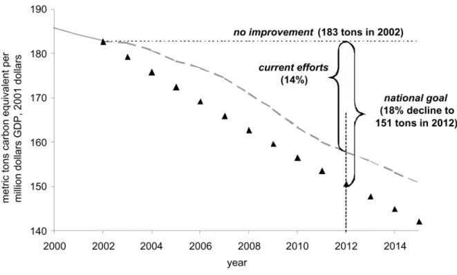
The implied change in emissions is shown in Figure 1 (White House, 2002). While the US Administration anticipates meetings its target with voluntary programs, we find that meeting it will require a positive carbon-equivalent price. We achieve the intensity target with an economy-wide cap-and-trade system covering all greenhouse gases. We also assume that Protocol members fully use the agreed sinks allocated under the final agreement at Marrakesh (see Babiker et al., 2002), and that both Protocol
members and the US include in their cap-and-trade systems all of the non-CO2 greenhouse gases
identified in the Protocol.
We then consider a number of implementation variants. Focusing first on Japan, we consider a high economic growth or “Recovery” scenario (NoTradR) that is consistent with expectations for growth when Kyoto was signed but now looks unlikely considering recent experience. Given 1997-2003 economic performance, to achieve a 2010 GDP level like that projected only a few years ago would require a large and immediate economic turn-around, and continued rapid growth over the remaining six years. Next we consider the implications of omitting the transportation sector from the Japanese emissions cap (ExTran), and of the effect of a 30% reduction of nuclear Table 2. Scenarios
NoTrad No Emissions Trading among parties. Reference average annual growth in GDP for Japan of 1.7%, the US 3.2%, and the EU of 2.7% over the period 1997 to 2010. We assume an economy-wide cap-and-trade without CDM credits. The US is constrained to meet the Bush Administration intensity target (18% emissions intensity improvement from 2000-2010).
NoTradR NoTrad but with rapid economic recovery in Japan, with GDP growing at a rate of 2.6% per year for 1997 to 2010.
ExTran NoTrad but with Japan’s transportation (TRAN) sector exempted from the cap.
N-30 NoTrad but with Japan’s nuclear capacity reduced by 30% to reflect temporary shutdowns.
ExtEU Extended EU bubble that includes EU expansion countriesa
. Japan and other regions continue to
meet Kyoto targets with domestic, economy-wide cap-and-trade systems but do not trade with each other or ExtEU.
EUJ Extended EU bubble includes Japan
FullTrd Full trade among Annex B parties to the Protocol, without US participation.
a
Modeled here as including the EET EPPA regional group, dominated by countries that will become part of the expanded EU.
1 A different set of assumptions is made in Sections 4 and 5, where we decompose the factors contributing to
Figure 1. Bush Administration Intensity Target for the US (White House, 2002)
capacity (N-30), as might be realized if some level of shut-down were to recur during the Kyoto commitment period.
The next set of scenarios considers trading schemes focused on the EU. To approximate planned EU expansion, we create an extended EU bubble including the EET (ExtEU) region in EPPA. This trading system immediately allows the EU to access hot air in the EET. We then consider the implications for Japan if it can trade within this system (ExtEUJ).
3.2 Simulation Results
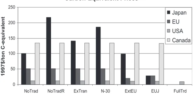
We have implemented the Kyoto targets for all Annex B parties including CAN, ANZ, EET, and FSU but focus our presentation of results on the four regions, the US, EU, Japan, and Canada. Figure 2 shows the carbon-equivalent prices in each region for each scenario. Notably, Japan’s carbon-equivalent price is much higher than the US, or the EU. Canada’s carbon price is the highest of the group. Canadian emissions grew strongly from the mid 1990s up to the present, and our reference forecast for Canada continues this growth. The US intensity target leads to a far smaller reduction than would its Kyoto target, but it still requires a $12 carbon price in the US in 2010 given our EPPA reference growth in emissions. The US price varies only by $1 to $2 across the scenarios, because we assume that the US does not engage in emissions trade with other regions. Similarly Canada’s carbon price varies little because we do not consider a case where Canada participates in emissions trading. (The policy variants do affect the US and Canada through trade in other goods, yielding only small effect on the carbon price.) The EU price in the NoTrad case is just above $50 per ton of carbon-equivalent while Japan’s price is
Carbon-Equivalent Prices
0 50 100 150 200 250NoTrad NoTradR ExTran N-30 ExtEU EUJ FullTrd
1997$/ton C-equivalent
Japan EU USA Canada
Figure 2. Carbon-equivalent Prices in Japan, EU, USA, and Canada
$100. Canada’s price is $135 per ton. Note, however, that in the ExtEU case, which is intended to simulate the likely result of EU enlargement to include several Eastern European Associates, the EU’s carbon-equivalent price falls to $21 per ton. Thus, in carbon-price terms the EU Kyoto-target, with EU enlargement, requires only slightly more effort than the Bush intensity target in the US. However, Japan’s effort, as measured by the carbon-equivalent price, is five to ten times that in the EU or the US, and Canada’s is still higher.
The scenario variants for Japan show that a partial cap-and-trade system that (1) excludes transportation (ExTran), or (2) must be carried out with less than full nuclear capacity in operation (N-30), or (3) is implemented under conditions of more rapid economic growth (NoTradR) could cause Japan’s carbon-equivalent price to increase by one and one-half to over two times. In some of the cases the carbon price exceeds that of Canada. Of course, similar uncertainties and implementation considerations are also present for the EU, the US, and Canada.
Access to international emissions trade, even if limited to the extended EU bubble, brings Japan’s carbon-equivalent price down to about $30. We estimate that full emissions trading, including full access to Russian hot-air, would reduce the price in the Annex B parties to essentially zero. The very low price under full trading among the parties, absent the US, is a finding of previous work (e.g., Babiker et al., 2002).
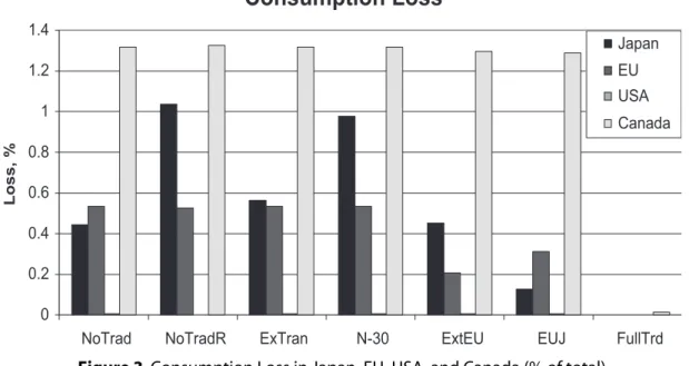
We turn now to the results in terms of economic welfare, measured in terms of consumption and stated in percentage terms, shown in Figure 3. This measure shows a much different picture of economic burden. The NoTrad case results in a somewhat greater burden on the EU than on Japan, with Canada’s cost by far the highest. The percentage consumption loss for Japan rises under the conditions described by the ExTRAN, N-30, and NoTradR cases, but still does not reach that of Canada. Of course the EU costs, even as a percentage, fall under ExtEU, and are thus much below Japan’s costs in all scenarios based on NoTrad.
Consumption Loss
0 0.2 0.4 0.6 0.8 1 1.2 1.4NoTrad NoTradR ExTran N-30 ExtEU EUJ FullTrd
Loss, %
Japan EU USA Canada
Figure 3. Consumption Loss in Japan, EU, USA, and Canada (% of total)
Beyond the very different carbon price and percentage loss effects, there are two additional paradoxical sets of results in Figure 3. The first is that the US has virtually no consumption loss in any of these cases—a result attributable to changes in goods markets (explored below). The second is that the costs of climate policy rise for EU when all of Europe trades with Japan
(ExtEUJ), compared to the EU costs when there is just trading within Europe (ExtEU). This result contradicts the common expectation that trading benefits both buyer and sellers of permits. Here, because the ExtEU bubble has a lower carbon price than Japan, expanding the bubble to include Japan will mean that ExtEU will be a net seller and Japan a net buyer of permits. Babiker et al. (2004) found a similar result: in a study of the implications for the EU parties of trading among themselves, the selling countries lost from entering a trading regime. In order to understand these paradoxical results we turn now to a discussion of what lies behind these different cost concepts. 4. COST CONCEPTS AND WHY COUNTRIES DIFFER
4.1 An Equal-Reduction Comparison
Japan is different from the EU, the US, and Canada in that its emissions intensity (emissions per dollar of GDP) is much lower, resulting from its higher efficiency in energy use and lower reliance on coal. Analysts have surmised that this difference is likely to affect Japan’s costs of meeting a carbon reduction target, relative to other countries, but they reach contradictory views of whose cost is larger. Some have argued that Japanese compliance would be most expensive because Japan is already the most energy efficient economy, and thus has few remaining options to further increase efficiency. Others have concluded that the Japanese economic loss due to Kyoto would be relatively small because, having the most efficient (and therefore relatively small) energy sector, an increase in the cost of that sector will have only a small effect on the overall national economy. In fact, these apparently opposite conclusions can both be true,
depending on the measure of cost. In addition, there are detailed aspects of economic structure that further help explain the apparent paradox.
To investigate the various factors that can lead to differences in cost among countries we first create a new set of scenarios that allows a focus on the energy efficiency question and other factors affecting the energy markets, isolating them from differences in emissions growth and from the effects of non-CO2 GHGs and sinks. Thus each region (including the US) is assumed to reduce its
emissions by an equal 25% from reference (approximately the same reduction required by Japan and the EU under Kyoto without emission trading). We also focus only on carbon, excluding the non-CO2 GHG gases and any consideration of sinks. These assumptions—no sinks and no access
to other GHGs—change the cost of the policy compared to the previous scenarios. The reduction is much larger than the Bush intensity target for the US, substantially raising the cost. It is a less stringent policy for Canada, so Canada’s cost is reduced compared with the Section 3 scenarios.
Table 3 shows how energy efficiency can be responsible for high costs (in terms of carbon price) or low costs (in terms of consumption loss). In terms of carbon price (Column 1), from highest to lowest the order is Japan followed by the US, then the EU, and finally Canada. Note that for a comparable percentage reduction in emissions from reference, Canada has a lower price than the others, whereas in the Kyoto results of Figure 2 Canada’s carbon price was much higher. This comparison shows that the carbon price in Canada under Kyoto is high because of the high reference growth in emissions, rather than from a lack of technological options.
In terms of percentage consumption loss (Column 2), on the other hand, the US cost is by far the lowest, less than 25% of that in the EU. Japan’s percentage consumption loss falls about midway between these two extremes. And Canada’s loss is very similar to Japan’s. Using market exchange rates (1997 US$), the economies of the US and EU are of comparable size, with the US somewhat larger, and thus the absolute consumption loss for the EU is roughly four times larger than the US (Column 3). Japan’s economy in 2010 is approximately 60% of the EU and the US. Even with the smaller economy, the absolute consumption loss is larger than in the US.2 Canada’s economy is smaller still, less than 1
/5 that of Japan’s.
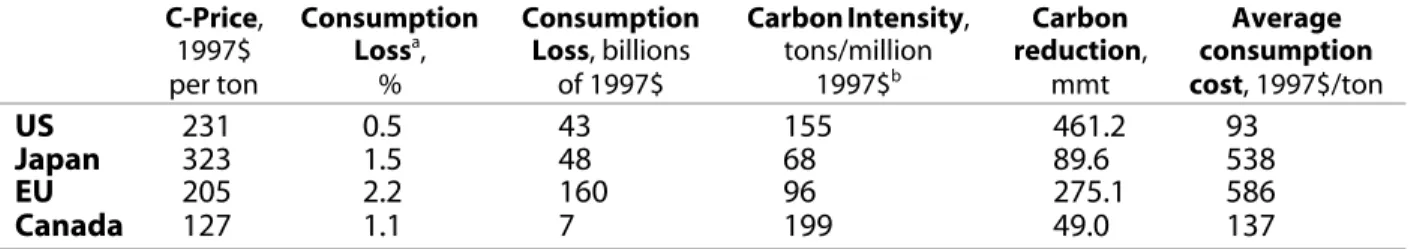
Table 3. Different Measures of Costs: 25% reduction from Reference of Carbon Only
C-Price, 1997$ per ton Consumption Lossa, % Consumption Loss, billions of 1997$ CarbonIntensity, tons/million 1997$b Carbon reduction, mmt Average consumption cost, 1997$/ton US 231 0.5 43 155 461.2 93 Japan 323 1.5 48 68 89.6 538 EU 205 2.2 160 96 275.1 586 Canada 127 1.1 7 199 49.0 137 a
Macroeconomic consumption loss as a percentage of total consumption.
b
GDP intensity: Carbon emissions/GDP.
2 It is important to note that these cross-country comparisons of the absolute cost (or size of the economy) depend
heavily on the exchange rate. Given that the GTAP base year data are for 1997, and we must balance trade flows with capital accounts, we use 1997 market exchange rates. The US dollar has fallen against the Yen and Euro since 1997, so these absolute comparisons would change, yielding a smaller relative reduction cost in absolute dollars for the US.
In fact, energy efficiency—or more specifically the difference in carbon emissions intensity (Column 4) resulting from a combination of lower energy intensity and less reliance on coal in Japan compared with the US or the EU—can explain this difference in consumption loss. Japan’s carbon intensity is less than one-half that of the US, and about 70% of Europe. On the one hand, Japan’s already emissions-efficient economy is the main reason its carbon price is much higher. For example, whereas the US, the EU, and Canada can fuel switch from coal to natural gas, reducing CO2 emissions for the same energy output, that option is limited in Japan. On the other
hand, the absolute reduction required in million metric-tons (mmt) of carbon is 70% larger in the US than in Europe even though the economies are comparable in size. In contrast, Japan’s reduction is only 20% of that required in the US and only 32% as large as that in Europe. Thus, while the carbon price is higher in Japan, any measure of total cost (cost per ton times the number of tons) will be proportionally less because of the smaller number of tons reduced. Canada is the most GHG-intensive of the four regions shown, and this fact is reflected in a required reduction in mmt’s that is more than 1
/2 that of Japan even though the economy is less than 1
/5 as big.
Furthermore, there is a deeper paradox, shown in Column 6. The average consumption loss per ton is the total consumption loss (Column 3) divided by the number of tons reduced
(Column 5). By this measure, the cost turns out to be very similar in Japan and the EU, but this value is about six times the cost in the US. Canada’s social cost is roughly twice that in the US but not nearly as high as that in the EU and Japan.
4.2 The Influences on National Cost
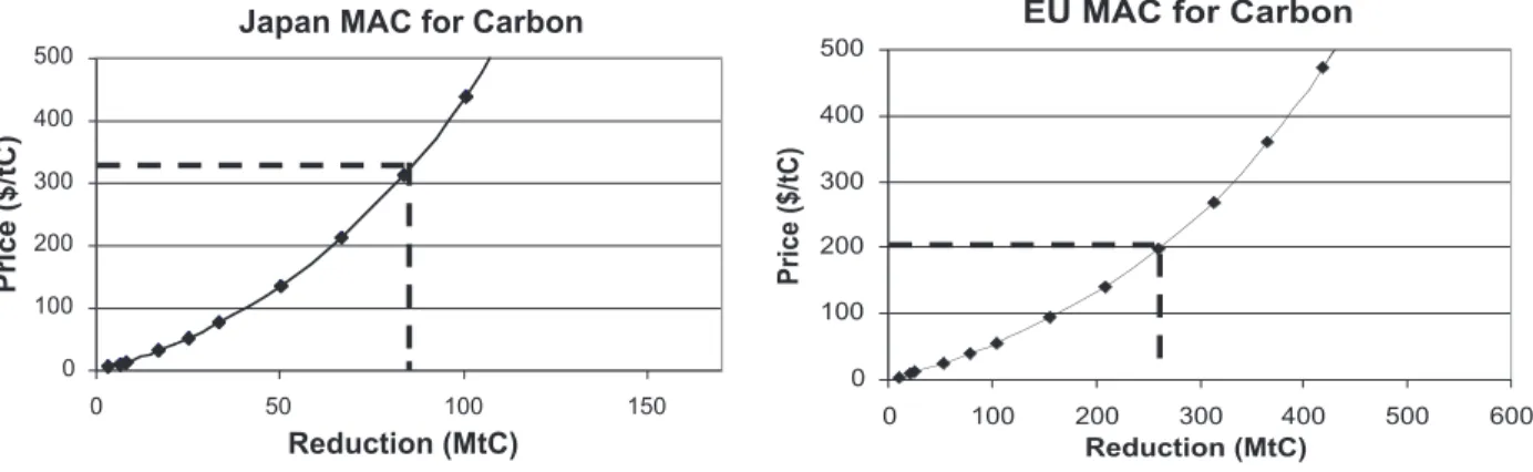
To explore these differences we need to consider in more detail how these different measures of cost are defined. First, the carbon price is a marginal cost, and an average cost will differ from the marginal. We can see this divergence with reference to a Marginal Abatement Curve, shown in Figure 4, for Japan and the EU. (These curves are derived using the EPPA model, again focusing only on carbon.) We derive the MAC by running the model with successively tighter emissions constraints and plotting the emissions reduction on the horizontal axis and the carbon price on the vertical axis.3
A dashed horizontal line is drawn at the price in Table 3 associated with a 25% cut from reference for each country. We then draw a vertical line from the point where it intersects that MAC to the horizontal axis, to confirm that this approach can accurately estimate the abatement quantity for each. Thus, such curves are a useful way to summarize the relationship between the carbon-equivalent price and emissions reduction (Ellerman and Decaux, 1998).
3
One complicating factor that immediately emerges is how to construct a MAC when multiple countries are involved in the policy. On can simultaneously tighten the policy gradually on all parties, one can assume that all other Parties are meeting a policy constraint and alter only the policy in the country for which one is constructing the MAC, or one can assume no policy in any Party except for the Party for which one is constructing the MAC. Because a policy can have spillover economic effects, the existence of a policy or not, and its severity, outside the country of interest will affect the emissions of that country and these different approaches to estimating the MAC will give somewhat different results. Here we have constructed the MAC for Japan assuming other Parties, including Europe, are meeting their Kyoto commitments and that the US meets the Bush intensity target goal. The same procedure is used for the other regions.
Japan MAC for Carbon 0 100 200 300 400 500 0 50 100 150 Reduction (MtC) Price ($/tC)
EU MAC for Carbon
0 100 200 300 400 500 0 100 200 300 400 500 600 Reduction (MtC) Price ($/tC)
Figure 4. Marginal Abatement Curves for Carbon, Japan and the EU
In a partial equilibrium analysis (i.e., focusing only on the energy sector and ignoring other effects) it is possible under some conditions to consider the area under the MAC curve, up to the required reduction, to be the total cost of the policy. The area is the sum of the marginal cost of each ton, the first tons costing very little (approaching zero) and the cost of the last tons
approaching the carbon price. We can take this total cost so estimated, and divide by the number of tons, to get an average cost per ton. Because the very highest cost reduction is the last ton of removal required to meet the target, the average cost derived in this way will necessarily be lower than the carbon price. If the MAC is bowed as in Figure 4, as it typically is when estimated from models of this type, then the average cost will be somewhat less than one-half of the
marginal cost. Absent an estimate of the full MAC, a rough approximation of the total cost of a policy can be constructed by assuming the MAC is not bowed in this way but is simply a straight line. The area is then the formula for a triangle:
Total Cost = 1
/2× P × Q, (1)
where P is the price of carbon, and Q is the quantity. Dividing by Q on both sides of Eq. 1 shows that, in this case, the average cost is exactly 1
/2 P. For the US, Table 3 shows that indeed the
average consumption cost per ton is somewhat less than one-half of the carbon price. The consumption cost is thus roughly consistent with an integrated area under the abatement curve.
But, this result does not hold true either for Japan or for the EU. In fact the average
consumption cost per ton is larger than the carbon price, and thus clearly cannot be an average of the marginal cost of each ton as represented in the MAC. Similarly, Canada’s average
consumption cost per ton is also above the carbon price. Integrating under the MACs for Japan and Europe, up to a 25% reduction, and dividing by the tons reduced, we find the average cost so derived is $150 for Japan, and $100 for Europe. As expected, the average costs calculated from the MAC are slightly less than one-half the carbon price. Thus, there are other considerations, not captured in the MAC, that increase the consumption cost of climate policy in these regions.
Before continuing our explanation of this difference, it now can be seen why, under these conditions, a region that sells permits can be made worse off, as happens to the EU in the
ExtEUJ case. In this example, a private firm at the margin in the EU sees the direct additional cost of reducing emissions to be $205, whereas a Japanese firm at the margin sees the cost as $323. The EU firm is willing to undertake reductions that cost $205 or more (let us assume $205) and sell them to the Japanese firm, and the Japanese firm would at the margin be willing to pay as much as $323 for these credits to avoid making the reductions themselves. We would expect an equilibrium market price to fall somewhere in between $205 and $323, and let us suppose it is $250. The EU firm thus profits $45 per permit by selling at $250 a reduction that cost it only $205. The Japanese firm benefits $73 per permit purchased by paying only $250 for reductions that would have cost it $323. But the average social cost of that ton in the EU is $586, and so the EU has a net loss from the trade, on average, of $586 – $250 = $336. On the other hand, Japan gains not only the avoided direct cost, but the avoided social cost of $538 – $250 = $288. In this example, the result of trading, summing across the two regions, is to reduce total consumption, because the gain of $288 in Japan is less than the loss of $336 in the EU.
The trading result for the ExtEUJ case depends on the divergence of the direct cost, as measured by the marginal abatement cost, from the social cost as measured by the consumption loss. Two factors are mainly responsible for this phenomenon. One is the interaction of the GHG policy with existing taxes (or subsidies) and the other is change in the terms of trade.4 A major difference for the US compared with the EU and Japan is that US fuel taxes are quite low, and thus we would immediately suspect that the fuel tax distortion effect is a major contributor to the high average consumption loss in Europe and Japan.5
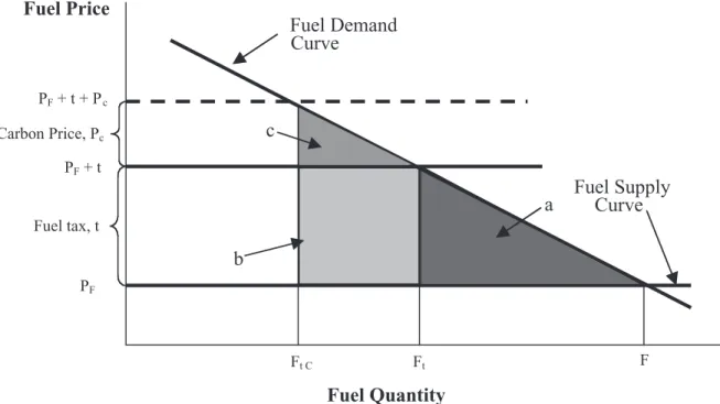
Figure 5 graphically depicts how existing energy taxes can increase the cost of a carbon policy. Here we represent the demand for a carbon-containing fuel, and its supply. The economic cost of a tax is the lost value of consumption of the good, less the cost of producing it. It is the area under the demand curve from the market equilibrium without the tax, up to the market equilibrium point with the tax. The cost of the fuel tax is thus the shaded area, labeled a. Adding a carbon price results in additional loss of the area labeled c, the direct economic loss associated with the carbon constraint, plus the area labeled b, the increase in the loss due to the original fuel tax.6
4
A country’s terms of trade is the ratio of the weighted average of its export prices divided by the weighted average of the prices of its imports. An increase in the ratio (more imports from the same physical quantity of exports) will increase welfare, and vice versa.
5 There can also be a further interaction with capital and labor taxes, but this does not occur in EPPA because of the
particular formulation of the model. Labor supply is fixed in each period, and thus taxes, or changes in the wage rate do not affect the quantity supplied. Thus, there is no deadweight loss with labor taxes directly represented in EPPA, and so with changes in the wage rate there is no additional deadweight loss from this source. Similarly, the formulation of EPPA as a recursive-dynamic model means that capital in a period is a fixed supply, determined by the previous periods capital, less depreciation, plus investment, with investment equal to the previous period’s level of savings.
6
To some degree the fuel tax may represent other externalities (e.g., air pollution, congestion) that are being managed using this instrument. We do not compensate for this aspect of the tax, and indeed European and Japanese tax levels are far above available estimates of estimated externality costs per liter of fuel.
Fuel Price Fuel Quantity Fuel Demand Curve Fuel Supply Curve PF Fuel tax, t PF + t + Pc PF + t Carbon Price, Pc Ft Ft C F a c b
Figure 5. Effects of Existing Fuel Taxes on the Cost of a Carbon Policy. The economic cost of
the fuel tax (t) added to the fuel price (PF) is given by area a. Adding a carbon constraint, with
a price of carbon (PC), raises the total fuel price, inclusive of the tax and carbon price, to
PF + t + Pc. With out the fuel tax, the economic cost of the carbon policy would be just the area
labeled c. But, the pre-existing tax means that the cost represented by the area b, in excess of the actual cost of the fuel, is also an added economic cost of the policy. A Marginal Abatement Curve (MAC) for carbon will include only area c.
If we consider that there is an area, here labeled c, under the demand for each fuel for each sector (and final consumption), the sum all of these areas for an economy will approximately equal the area under the Marginal Abatement Curve for carbon.7
Here we have drawn the demand curves as strictly linear, but as usually represented it will be convex with respect to the origin.8 This nonlinear relationship of demand to price gives rise to the curvature of the MAC. The important implication, however, is that if there are pre-existing energy taxes the area under the marginal abatement curve will underestimate the cost of a climate policy, and by a significant amount because the excluded cost is a rectangle whereas direct cost is approximately a triangle.
Another complication that arises with a carbon constraint is that it can interact with non-energy taxes further downstream in the economy to add to the cost of a carbon policy. Absent
7 To imagine this, consider a single fuel and a single market for that fuel. We could measure the fuel, instead of in
gallons or exajoules, in terms of the tons of carbon contained in the fuel. We could also compute the fuel price, instead of in dollars per gallon or exajoule, as the cost of the fuel per ton of carbon in it. The demand curve so transformed, and plotted as price rose from the initial market price without the carbon constraint would be exactly the MAC plotted as a ‘demand for carbon’, rather then the inverse, the willingness to do without carbon (i.e., abate).
8A fuel demand curve is not represented directly in a CGE model like EPPA, but is indirectly represented by the
representation of the production technology, usually as a Constant Elasticity of Substitution (CES) production function. To obtain the MAC from just the individual fuel demand functions, we required an uncompensated demand function that incorporates the changes in demand for downstream goods whose prices change.
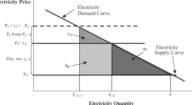
such downstream taxes, the own-price demand for a fuel (the demand curve one obtains by observing changes in demand when price changes)9 will represent the full economic loss in downstream markets. Consider, for example, the market for electricity produced using fossil fuels as shown in Figure 6. This graph is similar to the graph in Fig. 5. Here, however, the electricity price rises only indirectly because of the underlying carbon price on fossil fuels, and the specific rise will depend on the level of dependence on carbon-fueled electricity production and the ability to substitute away from these generation sources. Both the ability to substitute away in production, and the reduction in overall electricity demand shown here, will be part of the change in the fuel demand by electricity producers. So the economic loss directly due to price-induced reduction in electricity use, the area labeled cE, is already captured in the fuel
demand by electric utilities, and thus that loss is part of an area like c in Fig. 5. The area bE,
however, is not directly associated with the electricity price increase due to the carbon constraint, and thus is not captured in the fuel demand schedule, or as part of the area under a MAC.10 So,
Electricity Price Electricity Quantity Electricity Demand Curve Electricity Supply Curve PE Elec. tax, tE PE + tE+ ∆PE PE+ tE ∆ PE From PC Et E Et E C E aE cE bE
Figure 6. Effects of Existing Downstream, E.g. Electricity Taxes on the Cost of a Carbon Policy.
Downstream taxes can also add to the cost of a climate policy. An existing electricity tax, tE,
has economic cost represented by the area aE. Area cE is the economic cost resulting from
the change in the electricity price caused by the carbon policy. This economic cost is captured in area c in the previous figure and marginal abatement curve estimates. But the extra cost represented by the area bE. is not captured in the fuel demand curve or a MAC.
9 Distinguished from the unit demand function, which by assumption is calculated with a fixed demand for the good
produced using the fuel.
10 In this way, distortions throughout the economy can affect the economic cost of a policy as measured by
macroeconomic consumption loss. The interaction of distortions and GHG policy is not necessarily to always increase the cost. For example, a subsidy on the production of a fuel is a distortion, leading to greater use of the fuel than is economically efficient. A positive price of carbon that offset that subsidy could move the tax inclusive price closer to its efficient level, reducing the distortionary effect of the subsidy.
existence of these downstream taxes on products that use fuels in their production will add to the cost of an economic policy beyond that captured in the MAC.
Finally, changes in the terms of trade are another factor not captured in a MAC estimate of costs. We would highlight two reasons why these might change for particular countries as a result of climate policy. One is that many other countries in the world also are assumed to be undertaking greenhouse gas restriction. Whether or not a country takes such action, its terms of trade will be affected by the policies adopted by other parties. A second reason is that the
implementation of the policy in the domestic economy might, by itself, affect world prices. Often this latter possibility can be dismissed because the domestic economy is too small, relative to the world economy, to affect on world prices. We graphically show these effects below, including the case where the country is big relative to world markets.
Previous work by Babiker et al. (2000c) showed economic effects on developing countries, which imposed no greenhouse restriction, resulting from the climate policies of the Annex B parties. The effect occurred mainly through changes in the terms of trade. The effect of climate policy on the world oil price is the clearest example of this mechanism. A carbon policy in Annex B will reduce oil use in these countries, lowering world oil demand. There is then a consequent reduction in the world oil price. Oil importers (whether undertaking climate policy themselves or not) will gain from the lower oil price. Oil exporting countries will lose from this change because the price of a key export falls. For an oil importing country like Japan, which is also undertaking greenhouse gas reductions, this gain in the terms of trade will likely only partially offset the direct policy cost.
For other traded goods the direction of this effect is less clear. For example, parties taking on emissions targets will likely substitute away from energy intensive goods toward goods that are less energy intensive. This change alone would be expected to create a drop in the export price for these goods. But, among energy-intensive goods produced by different regions, Japan’s may be the least energy intensive. So, while the world demand for all types of energy intensive goods falls, the demand (and export price) for Japan’s energy intensive exports may rise. The net effect for a particular export or import good in a country thus will depend on its emissions
intensiveness relative to other goods, and the relative emissions intensiveness of that country’s version of the good relative to competing products made elsewhere. Because these different factors may operate in different directions, and depend on how Japan’s goods compare to goods in all other countries, it is possible to estimate this effect only in a model (like EPPA) that includes all of these relationships.
The possibility of either an increase or decrease in the demand for export goods is illustrated in Figure 7, where we show world demand as a horizontal line, as would be the case for a country too small to affect the world price itself. Even if demand were downward sloping, the gain or loss for the country is still a combination of a rectangular area (∆Px × X) and a triangular
area (1/2× ∆Px × ∆X). Where for an increase, X is X0 as shown in Figure 7 and ∆X = X +
– X0 and
+aX –aX Foreign Demand, Increase, Decrease X– Export Price +∆ PX – ∆ PX X+ X 0 Export Supply Export Quantity
Figure 7. Terms of Trade Effects on an Export Market From a Foreign Carbon Policy. We show
either an increase or a decrease in the demand for the export, either of which could occur because of the climate policy taken in foreign countries, and resulting in either a price increase of +∆PX or a price decrease of –∆ PX. An increase in demand results in a benefit to the
country represented by the area +aX, while a decrease in demand results in an extra cost
represented by the area –aX. Some export markets may gain while others may lose.
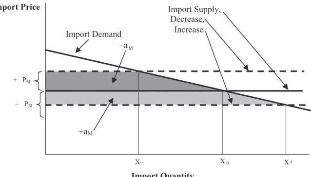
Similarly, the possibility exists that the price of imported goods might either rise or fall due to either a decrease or an increase in the supply of imports. This possibility is illustrated in
Figure 8, and the case of an increase in import supply to Japan (and a fall in price) is what has been found for the oil market. The world supply of oil does not shift, but the fact that other Annex B parties demand less, and thus more is available for Japan at a given price, is seen as a shift in the Japan’s oil import supply. Here, of course, a fall in the price is a gain to the economy because each unit of remaining import is less expensive, whereas a rise in the price of imports represents a loss to the domestic economy because now it must pay more for each unit. With much of the developed world (a major portion of the world economy) taking on a climate policy, some of these terms of trade effects are inevitable.
Terms of trade effects may also result from the climate policy taken in an individual country if it is big relative to the world economy or world markets for particular goods. Again, a country may experience a gain if the export price rises, a loss if its import price rises, or a gain if its import price falls, and these gains or losses are not captured in the MAC or fuel market estimates. In this case, the world price change is caused by a shift in the domestic demand or export supply. The shift in export demand could be up or down. The shift in export supply is almost certainly down, because all goods use some amount of fossil energy in production (directly or indirectly), and so their cost of production will rise.
+aM –aM Import Supply, Decrease, Increase Import Demand X– Import Price Import Quantity +∆ PM –∆ PM X+ X 0
Figure 8. Terms of Trade Effects on an Import Market From a Foreign Carbon Policy. Here we
show either an increase or a decrease in the import supply because of the climate policy taken in foreign countries. An increase in import supply reduces the import price by –∆ PM
and results in a benefit to the country represented by the area +aM, while a decrease in
supply raises the import price by +∆PM and results in an extra cost represented by the area
–aM. Some import prices may rise while others may fall. The import demand may also shift
because of the domestic policy.
For a small country, however, changes in the exports or imports induced by a policy change will have a negligible effect on the world price of these goods. Such a policy will affect the cost of producing export goods in that country, and therefore reduce the amount of exports, but that increased cost will be captured in fuel demand as represented in Fig. 4 or in a MAC. In the EPPA model, however, and in most CGE models like it, traded goods are treated as Armington goods. The Armington formulation imposes the notion that agriculture goods produced in Japan are somewhat different from the same goods produced elsewhere. That is, they are less than perfect substitutes, as represented in the model by an elasticity parameter. The Armington elasticities assumed in EPPA, and in CGE modeling of this type, are, however, typically quite high, on the order of 3.0, reflecting the fact that there is a large ability to substitute among like-goods from different countries. Thus, while the demand curve is not horizontal as in Fig. 7, there is little slope, and any rise in price will be small. Figure 9 illustrates that one would generally expect some slight welfare gain, partially offsetting the increased cost of producing these goods that is already captured in the MAC estimate. The export supply curve is also likely to have a shallow slope.
Export Price Export Quantity Export supply: before, after policy ∆ PX ∆ CX From P { C X X C aX bX X C P 0 Export Demand
Figure 9. Terms of Trade Effects From A Domestic Carbon Charge. With Armington goods, the
export demand for a country’s good is downward sloping, but with a high Armington elasticity the slope is small. A domestic carbon policy will increase the cost of goods using fuel to produce them (∆CX), with the increase depending on their energy intensity and ability to substitute away
from fuel use. This extra cost is already captured in the Marginal Abatement Curve. Not counted in the MAC is a partially offsetting benefit due to the rise in the price of the export good, the area labeled aX (∆PX × X C) less the area labeled bX, (1/2× ∆PX × (XC – X C P 0)]. That is, the extra price
earned for each unit still exported, less those for which the monopoly rents are less than the price increase.
5. DECOMPOSITION OF COSTS: NUMERICAL ANALYSIS 5.1 Analysis Method
We use the relationships identified in the previous section to estimate magnitude of each of these sources of cost in the four regions studied here. The marginal abatement curve (MAC) provides one basis for one measure of the welfare cost of a carbon policy, which we will call the “direct cost.” It can be estimated in either of two ways: as the area under the MAC estimated for the region as a whole, or as the sum across sectors of areas under MACs for each fuel. (The area of interest is illustrated by the letter c in Figure 5.) We compute the direct cost by both of these methods to confirm that the two estimates are approximately equal.
The sector-by-sector and fuel-by-fuel analysis also allows us to estimate the extra cost
attributable to pre-existing energy tax distortions. This is done by applying the tax level, available in the GTAP data set we use in our model, and the change in the quantity demanded for the fuel, which is available in the EPPA results. While the biggest distortionary effects are likely to occur in the fuel markets themselves (area b in Fig. 5), we extend the analysis into downstream markets as well, by evaluating the change in the quantity demanded in these markets in response to change in their supply (because of increased fuel costs) and the level of pre-existing tax distortions (area bE in Fig. 6).
We also evaluate the changes in the prices of exports and imports caused by climate policy by simulating EPPA with the policies implemented in all participating parties except Japan. To determine whether Japan itself has a significant effect on import and export prices, we compare these prices when all parties but Japan implement the policy with the case where all parties including Japan implement the policy. We expect the Japan-alone effect to be negligible, and, if so, we can directly estimate the terms-of-trade effect for each import and each export based on the graphical approach laid out in Figures 7 and 8, using actual estimated quantities and the change in price as simulated by EPPA. We then add up the various components for comparison with the regional level EPPA estimate. This total should approximately equal the total
consumption loss estimated directly in EPPA, and comparing the results achieved by different paths provides a check on the accuracy of the required approximations.
5.2 Necessary Approximations
The market-by-market method described above is based on a partial equilibrium approach. The EPPA model is a general equilibrium model, and so at best we can expect only to
approximate the consumption loss reported by the model by means of this decomposition analysis. In addition, the specific formulation of the CGE model will affect the decomposition results. Important features include which distortions are included in the underlying data set, how labor and capital markets are treated, and how the foreign accounts (trade and capital flows) are represented. Two of these issues merit special attention: the development of demand functions and the way the foreign sector is closed.
Demand Functions. One complicating factor that arises is that we do not have a direct estimate of the fuel demand function; we observe only the pre-and post-policy prices and quantities. These changes in quantity from pre- to post-policy conditions combine movements along a demand curve (the information we need) and shifts in the demand for a fuel resulting from price-induced substitution of one fuel for another (i.e., a shift in the Fuel Demand Curve in Figure 5). It is possible to analytically solve the production functions for the input demand equations. Given a production structure set in CES functional form, the unit input demand function (i.e., holding output constant) can be easily solved. The price elasticity of input demand (i.e., the slope of the demand for a fuel) is directly related to the substitution elasticity and the fuel input share. In the method described in the previous section, however, we are interested in full elasticity of demand that incorporates changes in sector output, not just the unit input demand elasticity. To solve analytically for this elasticity would require that we differentiate the entire nest structure of the model—a large task given the complex production structure in EPPA. Instead we have estimated the elasticity numerically by changing each fuel price in each sector independently and evaluating the change in quantity. We then use the formula for arc elasticity and the post-policy quantity, to estimate the change in quantity along the demand curve induced by the policy. That is, an estimate of the own-price elasticity of demand, ε*, is obtained:
ε* ^ – = ∆ ∆ Q Q P P 0 0 (2) Where ∆P–
is an arbitrary discrete change in price introduced into EPPA, ∆Q^
is the simulated quantity change, and Q0 and P0 are the initial quantity and price. Numerically, we use a large ∆P
–
to cover the range of price change we generally expect to result from the carbon policy. While the CES substitution elasticity is constant over any price, the own price elasticity of an input varies with its share even in the unit demand function, and downstream substitution possibilities offer more possibilities for a non-constant own-price elasticity. Thus, it is preferable to
approximate the elasticity over the actual price range we expect, rather than use an arbitrarily small price change to get a more precise estimate of the elasticity in the exact neighborhood of the initial price and quantity value.
We then simulate the carbon policy, and obtain ∆PC
, the price change (carbon price included) due to the policy. We can then estimate ∆QC as:
∆Q ∆P P Q C C = × × ε* 0 0 (3) This estimated ∆QC
will be that change in quantity due to the own-price response, which is the quantity relevant to the area under the demand curve that we need for our direct cost calculation.
This approach to the estimation involves the implicit assumption that the supply of fuels is perfectly elastic (i.e., horizontal as illustrated in Figure 5). Given that labor and capital are fixed in supply this is approximately the case, but there are supply-responsive factors in EPPA for the energy resources underlying the supplies of coal, oil, and gas. By not accounting for these supply-side effects we expect the loss as calculated by these components to be an underestimate of the loss as calculated on a national basis by the model (which does include these effects). This
numerical method is necessarily an approximation, and so we expect the sum of the decomposition components to at best only approximate the consumption loss estimated by EPPA.
Closure of the Foreign Sector. EPPA does not include a model of the monetary system or of foreign exchange rates (Babiker et al., 2001). In the model the current trade account is balanced in every period, on a global basis but not necessarily region-by-region. In addition, in the 1997 base year GTAP data set there are inter-country capital movements. These latter flows are zeroed out in the model, but only gradually over several decades. As a result, in 2010 there are
international monetary flows in the model that, while properly accounted for in the overall welfare analysis, will not be fully reflected the measures of direct cost, distortion and terms-of-trade effects as calculated by the methods described above. We have extracted these flows, country by country, from the EPPA results, applying needed corrections for the welfare effects of policy induced price changes, in order to adjust these flows for their domestic purchasing power.
5.3 Numerical Results
Table 4 contains the results of the decomposition for the 25% reduction scenario in Table 3. Shown there are the decomposition components: the direct cost, the cost attributable to
distortions in the fuel and downstream markets, and the terms-of-trade effect divided into two components: the sum of effects for all imports and exports except crude oil, and a separate effect of the change in the world price of oil imports or exports. Finally, there the correction for capital flows. The calculated correction for capital flows ranges from 0% to 2% of the overall welfare cost. The magnitude of these effects depends on the specific closure of the foreign sector in EPPA. Further investigation of these effects beyond the distortion and direct costs, and how they depend on model formulation, would be useful. We then compare the sum of these components with the estimate of consumption loss we obtain directly as an output of the EPPA model. We also compare the direct cost from this decomposition with our estimate of the area under the national MAC produced by the model.
First, we offer some general observations on the completeness of the decomposition. As expected, the sum of our decomposition elements is somewhat less than the model’s national consumption loss estimate—leaving, depending on the region, between 12% and 21% of the cost unexplained. In part this difference may arise because we have assumed a flat supply curve when in fact it is upward sloping in resource markets, and there may be other interactions we have not fully accounted for. While the part of the consumption loss unexplained by our decomposition is not negligible, the estimated components do explain a substantial amount of the loss. Also note that the direct cost and MAC cost estimate are very close, except for the US. Combined with the that we underestimate the consumption loss in all cases, the results further suggest that most of Table 4. Decomposition of 25% Reduction in Carbon Scenario
Japan EU US Canada Decomposition Component Direct Cost –11.23 –23.38 –42.51 –2.72 Distortion Cost –28.16 –108.74 0.27 –3.05 Terms-of-Trade Oil Market 0.40 1.09 2.76 –0.06 Other Goods 0.31 2.40 0.71 0.29
Correction for Capital Flows 0.66 0.35 0.91 0.02
SUM –38.02 –128.28 –37.86 –5.52
Comparison to EPPA Result
Consumption Loss –48.23 –160.08 –43.04 –6.71 Unexplained by Decomposition –10.21 –31.80 –5.18 –1.19
% Unexplained 21 20 12 18
Comparison to MAC
MAC Area 10.96 22.94 42.50 2.66
Difference from Direct Cost 0.27 0.44 0.01 0.06
the difference is due to a failure to account for all sources of loss, with the omission of supply side effects being the primary candidate. These results give confidence that we can compare the decomposition components across regions and scenarios even though we are do not account for all of the EPPA-estimated costs.
The results show that a big difference among parties is the distortion cost. For Japan and Europe it is several times the direct cost, while for the US is trivial. In Canada, the distortion cost is about the same size as the direct cost. Even though Canada has relatively low fuel taxes, the added distortion due to them can add up because it is non-marginal (a rectangular rather than a triangular area). Canada also looses from the oil market effects and, unlike the other regions, it sees almost no terms-of-trade benefits in remaining markets. The oil importing regions (Japan, the EU, and US) all gain in the oil market and by varying amounts due to terms-of-trade effects in other markets.
In many respects, the pictures for the EU and Japan are not very different, if account is taken of the different sizes of their economies. The relative magnitudes of direct cost, distortion, terms of trade, and trade effect for Japan are similar to the EU. One difference is that Japan, even with a smaller economy, gains almost as much as the EU in the oil market, which is not surprising given that Japan is completely dependent on imported oil. Canada differs from the others because it is an energy producer and exporter. And, because of the assumption of a flat supply curve we have not accounted for the domestic producer losses; this omission would be another reason why Canada’s costs would be higher, and may explain why overall we underestimate Canada’s costs by the largest percentage. The main reason for low consumption loss in the US is its relatively low fuel taxes. The US also gains substantially in the oil market because of the large amount of imports, and generally gains from trade changes.
6. CONCLUSIONS
Kyoto’s entry into force is still very much in doubt, with the domestic policy details of most parties still not specified, so possible costs to Japan or any other Party remain speculative. But as implementation of the Kyoto Protocol or policies like the Bush Administration’s intensity target for the US move forward, economic analysis of emission mitigation policies must begin to deal with more realistic implementation, representing national economies with the varying levels of existing taxes and economic distortions. As the set of issues addressed by these economic modeling studies has become richer and more complex, the definition of economic cost itself, and how it is estimated in economic models, has presented a puzzle, particularly to those outside the economic modeling community. Results can seem paradoxical: focusing on
carbon-equivalent price, Japan or Canada looks to be the high cost region, and Europe low-cost. But, in terms of welfare loss Japan appears low cost, Europe higher cost, and Canada higher cost still.
This paper demonstrates the implications of the use of different measures of cost, and explains why the relative carbon price among Kyoto parties may not be an accurate measure of the