Contact and free-gesture tracking for large interactive surfaces

(1)

Contact and Free-Gesture Tracking for Large

Interactive Surfaces

by

Che King Leo

Submitted to the Department of Electrical Engineering and Computer

Science

in partial fulfillment of the requirements for the degree of

Masters of Engineering in Computer Science and Engineering

at the

MASSACHUSETTS INSTITUTE OF TECHNOLOGY

June 2002

©

Che King Leo, MMII. All rights reserved.

The author hereby grants to MIT permission to reproduce and

distribute publicly paper and electronic copies of this thesis document

in whole or in part.

Author ...

Department of Electrical Engineering and Computer Science

May 24, 2002

Certified by...

...

.

...

Joseph A. Paradiso, Ph.D

Principal Research Scientist, MIT Media Lab

Thesis Supervisor

Accepted by...

Arthur C. Smith

Chairman, Department Committee on Graduate Theses

-SARKEP MASSACHUSMTS MTITU

OF TECHNOLOGY

JUL 3 1 2302

(2)

(3)

Contact and Free-Gesture Tracking for Large Interactive

Surfaces

by

Che King Leo

Submitted to the Department of Electrical Engineering and Computer Science on May 24, 2002, in partial fulfillment of the

requirements for the degree of

Masters of Engineering in Computer Science and Engineering

Abstract

In this thesis, I redesigned a Responsive Window that tracked the locations of phys-ical impacts on a pane of glass. To do this, I redesigned algorithms and boards, and utilized a DSP to do the signal processing. Tracking accuracy was significantly improved over the previous system. A study on radar rangefinding systems was also done to select the best radar system for integration with the Responsive Window. The applications for the system were realized, and debuted with great success. Thesis Supervisor: Joseph A. Paradiso, Ph.D

(4)

Acknowledgments

To Joe Paradiso for all his insight, intuition, and confidence in me. I thank him for giving me the chance to work for him. It has been a great, rewarding experience. To Stacy Morris for all her help and insights, as well her willingness to help review the previous incarnation of this thesis.

To Mats Nordlund for his insight and help with the Radar. To Steve Francis for his insight and help with the DSP.

To Axel Yamamoto for his timely resourcefulness with Panasonic transducers. To Mark Feldmeier, Josh Lifton, Hong Ma, and Nick Yu and all my colleagues and friends in the Responsive Environments Group for putting up with me and helping me when I needed help.

To all my friends for their patience, support and encouragement.

Finally, to my family for their encouragement, love and support. Without them, I would never have gotten this far.

(5)

List of Figures

1-1 Current hardware configuration for Responsive Window system. . . 19

2-1 Original PVDF with pickup . . . . 22

3-1 Flow diagram for determining knock position . . . . 28

3-2 "Bash" microphone glued to the window surface . . . . 30

3-3 Comparison of size between redesigned (left) and previous pre-amplifier board (right). . . . . 32

3-4 Preamplifier board with copper shielding . . . . 33

3-5 Internal view of housed electronics . . . . 34

3-6 External view of housed electronics . . . . 35

3-7 Flowchart for DSP software . . . . 36

3-8 Sampled waveforms for different tap types . . . . 37

3-9 DFT of sampled waveforms for different tap types . . . . 38

3-10 Ring down for a metal (top) and knuckle (bottom) tap . . . . 40

3-11 Absolute value GSM cellular phone noise picked up by the Panasonic EFVRT receiver and preamplifier (normalized) . . . . 42

3-12 Translation from point on window to pixel on projection . . . . 55

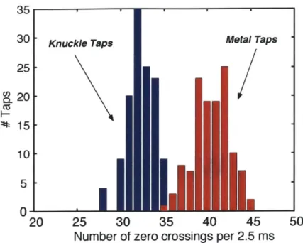
4-1 Histogram of knuckle and metal tap frequency . . . . 58

4-2 Piezo and dynamic responses to knuckle knock and bash . . . . 59

4-3 Granularity (for sample quantization) of Hyperbola Intersection algo-rithm for u=2000 m/s . . . . 60

(10)

4-4 Zoom of granularity of Hyperbola Intersection algorithm for u=600 m/s 61

4-5 Estimated positions for metal taps at five positions for 1 cm glass . . 62

4-6 Estimated positions for knuckle taps at five positions for 1 cm glass . 62 4-7 Estimated positions for metal taps at five positions for

4

inch glass . 63 4-8 Estimated positions for knuckle taps at five positions for 1 inch glass ₄ 64 4-9 Estimated positions for metal taps at five positions for (sensors 35 cm from corner)

4"

glass . . . . 65

4-10 Estimated positions for knuckle taps at five positions for (sensors 35 cm from corner)

4"

glass . . . . 66

4-11 Rays of energy leaving a point source in an inhomogeneous medium 68 4-12 Relative signal height vs. distance . . . . 70

5-1 Different window sensor placements: placement 1 - blue; placement 2 - red; placement 3 - black . . . . 78

5-2 Comparison of frequency components for different sensor placement. placement (1) (top) versus placement (2) (bottom) . . . . 81

6-1 Using the Saab Tank Radar Pro as a radar rangefinder . . . . 86

6-2 The commercial use for the Saab Radar Tank Pro . . . . 87

6-3 Micro-Impulse radar . . . . 88

6-4 Doppler radar developed at the MIT Media Lab . . . . 89

6-5 Doppler radar measurements . . . . 90

7-1 Interactive Drawing Exhibit at the Ars Electronica Museum . . . . . 94

7-2 Close-up of Interactive Drawing Exhibit . . . . 95

7-3 "A Telephone Story" Exhibit opening screen . . . . 97

7-4 "A Telephone Story" Exhibit in action . . . . 98

7-5 Storefront Display at American Greetings . . . . 99

7-6 Storefront display at American Greetings . . . . 100

7-7 Setup for the Interactive Window at SIGGRAPH, 2002 . . . . 101 10

(11)

7-8 Sample graphics for Interactive Window . . . . 102

B-1 Schematic for pre-amplifier board . . . . 110

B-2 Layout for pre-amplifier board . . . . 111

B-3 Schematic for analog signal conditioning board . . . . 112

B-4 Layout for analog signal conditioning board . . . . 113

B-5 Schematic for power supply auxiliary board . . . . 114

(12)

(13)

List of Tables

4.1 Table of knock statistics for inch window with sensors closer to Center 65

4.2 Table of knock statistics for - inch window with sensors further from₄

(14)

(15)

Chapter 1 Introduction

1.1 Problem Description

The quest to create interactive rooms has inspired much interest by the research community [1]. Indeed, many groups across the US work towards the greater goal of one day being able to live in a "smart" house fully facilitated by the use of computers and the latest technologies. As an example, there are advantages in making sensors which can be easily retrofitted to surfaces already available in homes easily retrofitted with sensors to make them interactive. Many windows have already been retrofitted with anti-theft systems. After all, the more information a computer has about its environment, the better it can aid the user. In this thesis we discuss methods for creating an interactive system from already in-place surfaces. This system would be able to generally monitor the user's position and activity within a given area, and feature a large, accurate, tracking surface for detailed interaction.

1.2 Prior Work

In 1998, Ishii and Paradiso collaborated to create a project called Ping Pong Plus

(16)

were correlated to where the ball had bounced on the table, allowing the players to attain a higher level of engagement. The tracking mechanism used in PP+ consisted of distributed microphones, and used a simple time of flight analysis to determine the position of the bounce. In this way, the ping-pong table was made into an interactive surface. Naturally, this straightforward technique could be expanded to other continuous surfaces, most notably glass.

The use of glass as an interactive surface is appealing in many ways. First and foremost, it is one of the most common elements in society today. Windows are in most any man-made structure, allowing many places to be easily retrofitted with an interactive surface. Second, glass is usually clear. Given sufficient throw, a projector and a screen can be placed behind the glass to allow images to appear, while never having parts of the image blocked by users, a problem found in most user interfaces that use a projector. In 2000, Paradiso et al. [3] proposed and demonstrated trans-forming large sheets of ordinary glass into an interactive surface capable of tracking the location of knocks via acoustic pickups adhering to the glass.

In 2001, Checka presented a more robust system of easily retrofitting pieces of glass into interactive surfaces [4]. Using piezoelectric polyvinylidene fluoride (PVDF) strips to pick up flexural bending waves created by users knocking on the glass, the system was able to roughly track and process the user input. The system was demonstrated by converting an ordinary conference room wall into a fully interactive web browser. However, there were a few potential drawbacks to this approach that prevented it from practical deployments. Most notably, the use of the interpretive language MATLAB and a commercial A/D PCI card to process the knocks caused considerable "dead time" of the system, and therefore limited the user's rate of input. Also, the use of a 3rd-order coordinate calibration model caused some points to be more significantly inaccurate than others. Finally, the system was limited to knocks made by human knuckles. This system was incapable of differentiating many different types of inputs, such as the difference between higher frequency metallic knocks (via

(17)

metallic objects like rings and keys) and more conventional human knuckle-based knocks. This is crucial for tracking knock position because the wavefronts from these types of knocks travel at very different velocities because of the dispersive nature of the glass. This system was also unable to correctly discern valid knocks which produce reliable coordinates from poor knocks that produce unreliable coordinates and false triggers caused by external sources such as pickup from cellular phones and sharp sounds like loud, nearby hand clapping or door slams. Finally, the system was only interactive in two dimensions, lacking the ability to have depth perception. Such an ability would seem to be a very useful feature, since it would provide an additional dimension's worth of information for the system to use. The screen, for instance, could respond differently as users approach.

1.3 General Overview

In this thesis, the Responsive Window system presented above was modified so that it became faster, more robust, more accurate, and produced more features. Changes ranged from rewriting the tracking and signal processing algorithms to modifying the hardware used in the system. In addition, a second system of sensor input was in-vestigated: a low-power range-finding radar, which would allow for a third dimension depth of detection. The addition of a system could add robustness to the interactive window system by monitoring nearby human presence, providing an entirely new level of interaction.

The system described by Checka [4] has been modified in several ways. First, the piezoelectric PVDF foil strips were replaced by piezoceramic microphones (Panasonic EFVRT series) which are less noise-sensitive [5]. These sensors were glued to the glass and covered by a shield box, reducing the total amount of electromagnetic pickup noise introduced into the system. An Analog Devices digital signal process on (DSP) replaced the National Instruments Card with MATLAB for data acquisition

(18)

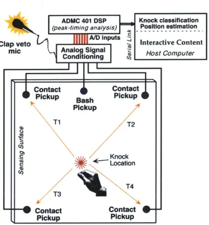
and the differential time-of-flight analysis. Figure 1-1 shows the current hardware configuration for the system.

Two extra microphones, labeled "bash" and "clap" were used to provide addi-tional information to the system. The bash microphone and circuitry which consisted of an electrodynamic microphone with a gain stage and lowpass filter was used to cleanly detect low frequency "bashes" (under 300 Hz; i.e. hitting the glass with the palm of the hand), since the piezo-electric pickups had a poor frequency response for low frequencies. The "clap" microphone was used to veto ambient noise from the sur-rounding off-window environment that falsely triggered the system. It was mounted in the air, instead of on the glass. Its analog signal conditioning involved several gain stages, a peak detector and a bandpass filter. By detecting when a large amplitude existed on the clap veto microphone, the system was able to use this information to reliably veto most of the false triggers to the system.

The analysis algorithms were substantially changed for improved performance and real time operation. A heuristically-guided chi-squared estimation was used to select which portions of the waveform most closely matched each other, so that those portions could be cross-correlated to fine-tune the accuracy of the values used for time-of-flight analysis. An iterative algorithm implicitly solved the problem of finding the intersection of the two hyperbolas defined by the time-of-flight values. This was done by matching the differential time-of-flight values by minimizing the error over the x-coordinate and the y-x-coordinate separately via a logarithmic search. The algorithm also counts the number of zero-crossings in the waveforms over a certain period of time. This simple frequency analysis was used in conjunction with the time-of-flight values in a nearest neighbors algorithm [6] to determine the dominant frequency of the flexural wave, thereby providing the correct speed of the waveform, a necessary value for correct calculation of the knock position.

In order to make the system aware of a third dimension, it will be augmented with a simple, low-power range-finding radar that looks through the surface of the

(19)

ADMC 401 DSP Knock classification

(peak -timing analysis) Position estimation

A/D Inputs

Clap veto Z Interactive Content

Mic Analog Signal Host Computer

.) HotCo '~1 C C C C Ci Contact Contact

Pickup Bash Pickup

Pickup Ti T2 Knock Location T3

17i

Contact Pickup Contact Pickup

Figure 1-1: Current hardware configuration for Responsive Window system.

(20)

glass. The radar will be monitored by the computer that drives the media content and video projector. This device also assisted the algorithm in several ways. First, in conjunction with the clap microphone, it reinforced the system to prevent false triggers, by instructing the system not to process a knock event if there is no user standing in front of the window. A second benefit from the range-finding radar was its ability to track and zone users as they moved about the window. Such information allowed the display to adjust its projection, evoking the feeling of interaction beyond knocks on a piece of glass, thus allowing users to fully immerse themselves in the window.

(21)

Chapter 2 Background and Motivation

2.1 The Previous Responsive Window Prototype

The previous system developed by Checka [4] described a system that employed polyvinylidene fluoride (PVDF) as contact sensors to track acoustic impacts on the window. Strips of PVDF backed with foam were mounted on a small PCB board that amplified the acoustic signals to increase the signal to noise ratio. This is shown in shown in Figure 2-1. Tiny nuts were then precisely super glued to the surface of the glass at desired locations and used to screw mount the board. The PVDF strips were thus tightly pressed against the glass and were able to pick up flexural waves originating from user input.

The acoustic waveforms created by knocks on the glass were amplified by the PCB board and sent through analog signal conditioning to remove high frequency components. After this, the signal was digitized by a National Instruments NI-6024E Data Acquisition Card and processed by MATLAB on a PC to discern the position of the acoustic impact on the glass. The algorithms used to derive position consisted of a third-order fit based on time-of-flight information obtained using cross-correlation analysis. The third order fit was based on data gathered via calibration. Calibration consisted of knocking on twenty known positions on the glass, and calculating the fit

(22)

Figure 2-1: Original PVDF with pickup

over these twenty variables.

When using the third order model, the system achieved an accuracy of less than a 5 cm standard deviation from the knock positions, when the knocks occurred on the calibration points. Checka also described a method for calculating time of flight from a simple rising edge analysis, which produced a 10 cm standard deviation from the knock position.

2.2 Motivation

In the quest for a system that can be responsive to user input, we wanted to create a system that responded to acoustic impacts in real-time, as well as to a wider spectrum of user input, unconfined to the rigors of meticulously setting up a precise calibration system. We also desired a system that improved on accuracy and/or precision. Lastly, we wished to create a more robust system, which was less likely to be fooled by fake input (i.e., ambient noise and other false triggers), while still being responsive in some way to all types of valid user input.

(23)

2.2.1 Real-Time Response

The use of MATLAB as the signal processing tool, was beneficial for developing algorithms, due to its close-to-infinite precision arithmetic. However, depending on MATLAB running on a PC is a poor choice to employ in creating a system that needs to process information at a rate better than the maximum rate of human knocking (5-10 Hz). In the previous system, using the NI-6024E and MATLAB setup incurred approximately one to two seconds of delay before a response was shown on the screen. To improve on this delay, some of the algorithms were implemented on a digital signal processor (DSP), as described in this thesis.

2.2.2 Increased User Input Spectrum

The previous system was only able to track knocks created by an impact with one knuckle. This was because the calibration knocks used to calculate the coefficients for the forward determination scheme in the third order fit were all knocks using a single knuckle on each calibration point of the glass. Using multiple knuckles or different sections of the hand, including the palm, the fist, and fingernails often led to inconsistent results; thus the previous system could only determine knock position caused by knocks made with the knuckle. The new system was designed to be able to track impacts caused by other sources, such as metallic taps from rings and keys. The system was also able to track and/or respond to a wider range of knuckle knocks. This is vital, as people will knock in any fashion in a public venue, and one cannot reasonably expect them to be highly constrained.

2.2.3 System Robustness

The previous system ran on Windows 98, and the machine required rebooting every day. Without rebooting once a day, continual knock estimation would fail, because the NI-6024E and MATLAB combination would stall and stop processing taps, causing

(24)

the system to freeze. A migration to a digital signal processor (DSP) for signal discretization and part of the signal processing easily improved system robustness by eliminating the signal processing done on the PC. Second, the sensors would also pick up random noise before the amplification stage. This problem was solved by changing the sensors and placing a shield of copper on the pre-amplifier board. Finally, the PVDF sensors would fall off easily, as the strength of their attachment to the glass relied upon the screw connection between the pre-amplification PCB boards and the nuts glued to the glass. By changing the type of sensors to a cheap, commercially produced device (piezoceramic telephone receivers, found to be superior in performance to the other pickups tested for this purpose), it allowed the sensors to be super-glued to the glass, thereby eliminating the mechanical instability of Checka's

"pinched" sensors.

2.2.4 System Portability

The previous system also did not lend itself to portability. The requirement to have a PC with an open PCI slot for the NI-6024E card, as well as needing prototype analog electronics did not allow the system to be easily brought from place to place for display. The complicated setup and extensive requirements for different software made the system less portable. It was also desirable to build a system that could be eventually manufactured cheaply (at a cost of less than 100 per unit). The use of the $3000 NI-6024E data acquisition card prohibited this requirement. Therefore, a DSP was used for signal discretization and initial signal processing.

2.2.5 Self Calibration

Another requirement for the new system was that it should have an easy to use user interface (UI) that would allow any user to calibrate the Responsive Window system. Because every sheet of glass could potentially have different characteristics, a program was needed that was versatile and allowed the user to easily calibrate the system.

(25)

2.2.6 Free Gesture Tracking

To allow for free gesture tracking, radar rangefinding systems were investigated for integration into the Responsive Window. This integration will allow the system to react not only to two dimensional input on the sheet of glass, but also the third dimension of depth away from the surface. Doing so broadened the spectrum of applications for the system.

(26)

(27)

Chapter 3 Responsive Window System Design

3.1 Design Overview

This section describes the Responsive Window system in four parts: Hardware Design, DSP Software Design, PC Software Design, and Window Calibration.

The hardware design for the Responsive Window consisted of a redesign of the analog signal conditioning board, as well as a design of the digital components, and the physical implementation of the system (i.e. where the sensors are placed on the window, and other physical structures used to improve robustness). The PVDF strips were replaced with Panasonic piezoelectric receivers. Two more sensors were

introduced to the system - a crystal microphone for vetoing high energy noise that

can falsely trigger the system, and an electrodynamic microphone for detecting low frequency "bash" impacts that did not get picked up well by the Panasonic receivers. The pre-amplication boards were designed to increase bandwidth, to prevent acci-dental destruction of delicate analog parts, and to make them modular. The DSP chosen to do the signal processing and signal discretization was the Analog Devices ADMC401 DSP chip, which has the ability to interface with a computer via a serial cable link.

(28)

Deter-Calibaion

Figure 3-1: Flow diagram for determining knock position

mination Code, and Calibration Code. The Calibration Code calculated parameters

to be used by the PC Knock Position Determination Code. The entire knock position determination software design for the Responsive Window required both DSP and

PC code. The DSP code extracted useful characteristics for determining knock type, as well as time-of-flight information between two predetermined pairs of sensors. The PC knock determination program, was written in C++, and used parameters obtained from calibration code and parameters from the DSP to calculate the knock position.

Figure 3-1 shows the flow diagram for the Responsive Window knock position deter-mination.

3.2 Hardware Design

The hardware redesign was done by using a bottom-up approach. First, the appro-priate sensors were chosen to replace the PVDF strips. Then, the pre-amplifler board was redesigned. Next, the analog signal conditioning board was redesigned to include channels for all the microphones. Then, a DSP was chosen, and a board was made to power different sections of the hardware, followed by physical enclosures for the

(29)

system. Finally, sensor placement on the window was considered.

3.2.1 Replacing the PVDF Strips

First, different types of microphones were investigated to replace the PVDF strips, since the PVDF strips did not have uniform frequency responses. Also, the mount-ing for the PVDF strips allowed various amounts of background noise to enter the system, depending on how tightly strips were pressed against the window. Therefore, manufactured transducers were investigated, including microphones, speakers and other sensors. The final choice was a Panasonic piezoelectric cellular phone receiver (EFVRT series). The receiver had a 300-5000 Hz range for its frequency response, which covered a portion of the frequencies of the knocks of interest. This Panasonic receiver had the best performance across all types of knocks compared to all other transducers tested for this application. A low frequency impact "bash" microphone was used to complement the Panasonic receiver in the very low frequency range, where bashes produced the most response. However, the Panasonic receivers were suscep-tible to interference from cellular phone transmission signals when cellular phones which used the GSM standard were very close (e.g. a few feet), so this flaw was compensated for in the DSP code.

3.2.2 Low Frequency Impact Microphone

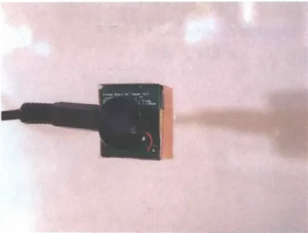
To allow the system to respond to low frequency "bash" impacts (such as those from the fist of a hand), a fifth microphone was used. An electrodynamic microphone was chosen because it responded well at lower frequencies. In order to be maximally responsive in the lower frequency range, the microphone had to be glued with only its diaphragm stuck to the window. Thus, in order to allow the microphone to operate in a stable manner (without falling off), we had to epoxy the center of the diaphragm to the window, and cantilever the mass of the microphone while strain-relieving the cable. Figure 3-2 depicts the electrodynamic microphone with its diaphragm glued to

(30)

Figure 3-2: "Bash" microphone glued to the window surface

the surface of the glass. The resultant assembly was resonant at the low frequencies excited by a bash. This microphone was conditioned by a circuit that used simple analog peak detection to determine whether or not very low frequencies had been detected. Figure B-3 in Appendix B diagrams the final circuit used.

The peak-detected signals from the low frequency impact microphone were used to determine if a "bash" event had occurred that was beyond the frequency response range of our piezoelectric receivers.

3.2.3 External Noise Transient Veto Microphone

The quest to allow for a broad user input spectrum also allowed the system to be susceptible to external events that could falsely trigger an event. The main source of false triggers came from high-energy transient signals, such as hand clapping. The energy of hand clapping can couple into the glass and cause the receivers to falsely pick them up as knocks. Therefore, we placed a sixth microphone in the air so that the system could tell if the signal was stronger in the air or in the glass, thereby indicating the origin of the trigger. A simple crystal microphone was used that had a very nice frequency response to the types of sharp, transient signals that created

(31)

false triggers.

Analog components were designed to properly filter the signals from this trans-ducer. Figure B-3 diagrams the final circuit. A high gain stage was provided for the signal, since an amplifier board was not used for this microphone, and out-of-band noise was filtered.

3.2.4 Redesigned Pre-Amplifier Boards

In order to minimize induced noise and electromagnetic pickup, the first stage of the preamplifier was mounted right at the transducer. The original pre-amplifier boards [4] were built with two goals in mind. The first was to allow the boards to be screwed onto nuts crazy-glued onto the surface of the window, so that the sensors could be removed without damage. The second was to improve the signal to noise ratio (SNR), by amplifying the signal before it was transmitted to the main board.

A 3-conductor cable using a mini-stereophone jack coupled the power, ground, and output signal to the preamplifier boards. When the stereophone cable was physically plugged into the pre-amplifier board jack, there was a brief moment when the signal out was shorted to ground. The previous setup thus allowed full power to be dumped out of the output of the preamplifier IC, an OP162, into ground. Hence, if this was done while power was on, it would sometimes result in the OP162 burning up. In order to limit the output current, we placed a small resistor (330 Q) was placed in series with the output to the OP162.

Also, since the piezoelectric microphones required a high impedance input, R4 and R5 were increased to 2.0 MQ in order to get a better signal from the output. Finally, in order to provide modularity, the board was designed so that it could be used for microphones that required either a low or high impedance front end. Figure B-1 from Appendix B shows the new schematic for the pre-amplifier board.

The area board was decreased by 45%, so that the amount of stress and torque on the sensor was reduced. The use of the smaller board size allowed for the use of

(32)

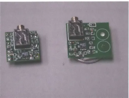
Figure 3-3: Comparison of size between redesigned (left) and previous pre-amplifier board (right).

a wider range of sensors, (i.e., sensors with smaller footprints). Figure 3-3 compares the sizes of the two boards.

To reduce the amount of noise pickup at the preamplifier stage, a physical shield made from copper siding material was fitted on top of the preamplifier board. Fig-ure 3-4 depicts a board fitted with the copper shield.

3.2.5 Digital Signal Processor

The digital signal processor (DSP) that was chosen had to meet several requirements. First, the DSP had to be able to sample on at least six channels, allowing it to sam-ple the inputs from the four contact microphones, plus the two other microphones. Second, the DSP needed a sample rate well above the Nyquist frequency. The Pana-sonic EFVRT receivers had a frequency range up to 5 kHz, so to properly sample the wavefront signal, the DSP had to have a minimum sampling throughput of 50 kHz per channel. Third, a good data resolution of at least 10 bits was desired. Finally,

(33)

Figure 3-4: Preamplifier board with copper shielding

the DSP needed to have a serial output connection to allow the DSP unit to easily interface with most computers, either via a USB serial port or a legacy serial port.

At the time of the DSP selection, the only readily available solution that met all

of these requirements was an evaluation kit from Analog Devices - the ADMC401

Motor Controller Kit. The ADMC401 kit had eight channels of inputs, a sampling rate of 50 kHz, 12-bit resolution, and a serial port interface.

3.2.6 Sensor Window Placement

The four main contact sensors were placed so that each sensor was not too close to the window edge, to minimize the effects of reflections from the closest window edge which could contaminate the wavefront arrival. Because the highest dominant frequency traveled at speeds ranging from 1200 m/s to 3000 m/s (depending on glass thickness), a 50 kHz DSP sampling rate was insufficient to allow for sensor placement in arrays. this would have allowed the position to be determined via a linear array of sensors with phase calculations. The best solution for our constraints was to place

(34)

Figure 3-5: Internal view of housed electronics

each sensor some constant distance from each corner. Chapter 5 discusses experiences with different sensor placements on the window and their implications.

The "bash" microphone was placed at the top center of the window. The elec-trodynamic microphone needed to be able to sense very low frequency flexural waves from its location. The "clap" microphone was placed in front, concealed out of view at the top of the display. This was so that users would not see the microphone, and deliberately try to trick the system into falsely triggering.

3.2.7 Physical Hardware Implementation

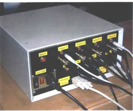
To protect the electronic hardware in the system, all the analog and digital com-ponents were placed inside a sturdy 11.5" x 8.5" x 5.5" aluminum box. Power was provided to the system by a ±5V power supply. A breakout board was used to dis-tribute various voltages required by system components, including 9V for the serial driver, 5V, and -5V for the analog and digital electronics. Figures 3-5 and 3-6 depict the internal and external view of the box.

(35)

Figure 3-6: External view of housed electronics

3.3 DSP Software Design

The DSP Code was used to extract features from the sampled waveforms, and send these features to the PC Knock Determination Program. The DSP code can be

bro-ken up into several parts - waveform normalization, trigger threshold, cellular phone

interference detection, zero crossing count, heuristic waveform selection, rising edge selection, and analysis of the signals provided by the "bash" and "clap" microphones. Figure 3-7 is a flowchart for the DSP software.

A dynamic trigger threshold on the window-mounted sensors controlled the point at which samples from the sensors would start to be processed. Next, any vetoes were derived to stop processing for false triggers, such as cellular phone noise. Events considered valid were then further processed to acquire a zero crossing count, and a heuristic waveform selection and rising edge analysis was performed to find differential time-of-flight parameters.

(36)

Figure 3-7: Flowchart for DSP software

characteristics of the waveforms sampled by the DSP.

3.3.1 Sampled Waveform Analysis

Figure 3-8 illustrates several types of the waveforms that can be obtained from various

impacts on a 143 cm x 143 cm, inch thick tempered glass, mounted on a wooden

frame. As the metallic taps produced a much larger response in the transducers, they tended to saturate more (although the most relevant initial wavefront remains linear.)

Hard, "metallic" impacts were found to excite higher frequencies than most knuckle impacts. This is evident not only from looking at the Discrete Fourier Transform

(DFT) of the sampled signals (with the DC gain subtracted out), but also from

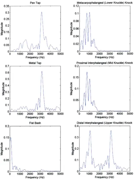
hear-ing the timbre of the sound made from the knock. Figure 3-9 shows the magnitude of the frequency response for the various waveforms shown in Figure 3-8.

There are two big peaks at around the vicinity of 1000 Hz for knuckle-based impacts, and one peak at 3200 Hz for metal-based impacts. Regardless of objects used for impact, it seemed that the only major frequencies that could be excited by users for this particular sheet of glass were located around 1000 Hz and 3200 Hz. Because of the

(37)

I Pen Tap 0 2 4 6 time (mS) Metal Tap 2 0 21 o 2 4 6 8 time (ms) Fist Bash 0 0 2 4 6 a fimne (MS)

Metacarpophalangeal (Lower Knuckle) Knock

2 0 -2 I" J -2 o 2 4 6 8 0 2 4 6 8 time (ms)

Proximal interphalangeal (Mid Knuckle) Knock

-1

0 2 4 6 8

time (ms)

Distal interphalangeal (Upper Knuckle) Knock

1

-1

0 2 4 6 8

time (ms)

Figure 3-8: Sampled waveforms for different tap types

-1

V 1, f

~RH

(38)

-Pen Tap 0.35 . '> ~Vid 1000 2000 3000 Frequency (Hz) Metal Tap

Metacarpophalangeal (Lower Knuckle) Knock 0.12. 0.1 0.08 &0.06 0.04 0.02 0 1 4000 5000 0.3 0.25 0.2 0.15 0.1 0.05 0 0 0.7 0.6 0.5 0.4 0.3 0.2-0.1 0 0 1000 2000 3000 4000 5000 Frequency (Hz)

Proximal Interphalangeal (Mid Knuckle) Knock 0.2 0.15 0.1 0.05, 0 0 1000 2000 3000 4000 5000 Frequency (Hz)

Distal Interphalangeal (Upper Knuckle) Knock

0.4. 1 0.3 0.2 0.1 0 0 1000 2000 3000 4000 5000 Frequency (Hz) 1000 2000 3000 4000 Frequency (Hz) 5000

Figure 3-9: DFT of sampled waveforms for different tap types

1000 2000 3000 4000 5000 Frequency (Hz) Fist Bash 0. 0.1 0. 0.0 2 5 5 ~jP ~ --I- - -- -- -- - - - -Z= kamwWagem

(39)

dispersive nature of the glass, different frequency components in the glass propagated through the glass at different speeds. Thus, calculating the velocity for both dominant frequencies became essential for determining knock position. Because the two peaks at 1000 Hz traveled at relatively the same speed, the average speed for knocks exciting that frequency range was used. Perplexingly, the distal interphalangeal joint (upper knuckle) knock has frequency content in both areas. In order to properly calculate the knock origin for the upper knuckle knock, a velocity associated to the frequency at 1000 Hz was used. This led to an algorithm for determining the difference between knuckle and metal knocks.

If the mean of each set of waveform samples was brought to zero by subtracting out initial bias, and took the absolute value of each waveform, "lobes" that represented the flexural waves caused by the impact were left. At some point the peaks of each lobe no longer increase in magnitude and the waveform appears to become "random." This "randomness" is mainly caused by the dispersive nature of glass, the nature of the impact excitation, and the reflections from the glass edges as the glass lapses into modal oscillations. Thus, in order to accurately find a good differential time-of-flight between two sensors, it would be easier to only compare "clean" sections of the signal where only one frequency component is dominant. This is a departure from the cross-correlation method that Checka [4] used. In the previous system, Checka performed cross-correlation on entire 8 ms samples of both signals. Here, this system seeks to increase precision by correlating specific sections of each sample which were more clearly from one dominant frequency.

3.3.2 Dynamic Trigger Threshold

In order to process knock events, it was important to know when the timing and the number of input signal samples were valid for processing. At first glance, this would seem easily determined by taking some amount of samples before and after a set threshold was reached; however, this method would lead to many false triggers.

(40)

Metal Tap Ring Down

I I I I I I

10 20 30 40 50

time (ms)

60 70 80 90 1]

KnucMe Tap Ring Down

10 20 30 40 50

time (ms)

)0

60 70 80 90 100

Figure 3-10: Ring down for a metal (top) and knuckle (bottom) tap

2 1 -1 -21 0 2 0 -2 0

(41)

Figure 3-10 shows the "ring down" effect for a knuckle and metal tap placed at the center of a 143 cm x 143 cm window with sensors placed 35 cm from each corner. The window could ring for over 0.1 seconds like a chime (depending on the kind of glass and the mounting), causing false triggers immediately after the correct, initial tap was processed. Therefore, a dynamic trigger threshold was implemented, so that the knock threshold would immediately rise in magnitude after an event was triggered, and thereafter slowly return to the original base trigger threshold. Since any new events of significant intensity are well above the "leftover" signal from the previous impact, a trigger using the artificially higher threshold would mean a fresh knock has occurred. Once triggered, 400 samples (8ms) were stored, consisting of 150 pre-trigger samples and 250 post-trigger samples for each of the four contact microphones and the clap microphone. Since the low frequencies arrive much later, an extra 600 post-trigger samples were stored for the slow-response, low-frequency impact microphone (for a total of 1000 samples). Triggers were caused by exceeding the threshold on any of the contact pickups or the bash microphone signals. They were not used by the

"clap" microphone, which only produces a veto.

3.3.3 Cellular Phone Noise

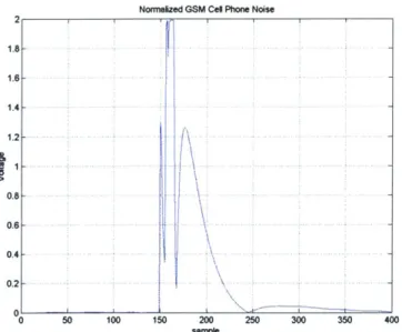
Because the Panasonic EFVRT series receivers and the preamplifier boards were sensitive to GSM cellular phone signals, the DSP was used to veto such signals. This was done by investigating the structure of the signals that which were picked up. Figure 3-11 shows the absolute-value waveform received for a common GSM signal.

The GSM pulse had a relatively sharp decay curve and was zero outside its pulse range. This was unlike a knock event, which took relatively longer periods of time to ring down. Thus, the DSP checks to see if the end of the sampled signal is at noise levels. This indicates that cellular phone signals, and not real knock events, are being picked up since the cellular phone signals decay much more rapidly.

(42)

Normwaized GSM Cel Phone Noise 2 1.8 -- 1.6- 1.4- 1.2-0.8 -0.6 -0.4 0.2 0 0 100 150 200 2 50 30 350 400 sampl

Figure 3-11: Absolute value GSM cellular phone noise picked up by the Panasonic EFVRT receiver and preamplifier (normalized)

3.3.4 Zero Crossing Count

A zero-crossing count was done before any waveform processing. This operation counted the number of significant crossings through the initial bias for the sampled waveform. A simple crossing count was done as follows:

(1) Calculate a threshold for noise +d and -e (d, e E R+), forming a transition band

of width d + e.

(2) Increment the zero crossing count every time the signal alternated sides of the transition region.

This method only counted the dominant frequency in the system, since signals which had a frequency component smaller than the width of the transition region had little affect on the zero crossing count. It resulted in a fairly accurate tally of the number of zero crossings at the dominant frequency, thereby estimating whether the dominant frequency was low or high. This was used as a very simple means to calculate the dominant frequency of the flexural wave, so as to select the correct speed of the

(43)

flexural wavefront.

3.3.5 Waveform Normalization

The initial bias was subtracted from the sampled waveforms, xa[n), before analysis was performed on them. This allowed all the sampled signals to be compared with each other without trouble. Because only differential time-of-flight analysis was im-plemented on a small frequency band, simple positive algebra could be used to avoid excessive use of absolute values on the DSP by finding the zero-referenced absolute value of the waveform. This is because the positive envelope for a given narrowband signal is approximately equal to its negative envelope.

The waveform was compensated by subtracting the initial bias in the signal (during the first fifty samples of the pre-trigger phase), and then the absolute value was taken

to get the new waveform,

sa

[n], as follows:

Ma[n] = IXa[n] -

50

Xa[i]| (3.1)

O<i<50

In order to reduce noise in the system, the signal was conditioned with a simple first order FIR filter to acquire the normalized waveform, c[n]:

~ a[n - 1] +i Ea[n]

C = na[n] 2 (3.2)

2

3.3.6 Rising Edge Detection

When trying to determine which samples of each waveform originated from the source at the same time, the simplest solution would be to look for the spot where the signal rises above a threshold in all four waveforms. This is called rising edge detection, since it looks at the first significant rising edge of the waveform. However, it was found that rising edge detection was somewhat inaccurate, especially for knuckle knocks. A low threshold was susceptible to noise, while a high threshold was susceptible to missing

(44)

rising edges due to attenuation of the signal. Knocks close to one sensor would have very different maximum magnitudes for the sensor that was close by compared to the sensor that was furthest away.

The method used here was to find the spot where the signal first surpassed of the maximum height of the sampled signal. From this point, the algorithm then backtracked n steps, before proceeding forward to find the first spot that rose above some lower threshold. In other words, in order to provide a more accurate rising edge estimate, a higher threshold was used first, preceded by a lower threshold crossing (in effect a double threshold level). The maximum n between thresholds was chosen to be 50 samples, an estimate for the length of two full cycles of the lower dominant frequency for the flexural wave.

None of these thresholds are related to the dynamic trigger threshold used in ac-quiring the samples and described in Section 3.3.2. However, since the lower threshold is a constant voltage (0.1V) above the maximum "noise" voltage in the pre-trigger phase, this method estimates the rising edge incorrectly less often than one cycle.

3.3.7 Heuristic Chi-Square Fit and Cross Correlation Method

While improving accuracy compared to the previous Responsive Window system for position determination, the rising edge method discussed in the previous section did not have good precision. One way to increase precision when using the rising edge method is to match the features (e.g. zero crossings and peaks of lobes) instead of

just the rising edge in the normalized waveforms,

za[in].

It would be ideal to perform signal processing on the parts of the sampled signal that are least affected by dispersion or reflections. Due to dispersion, zero-crossings in those affected parts of the wavefronts are not reliable markers for time-of-difference calculations. Because dispersion causes higher frequencies to travel faster, the earliest part of the signal consisting of the highest dominant frequency was examined, result-ing in the examination of a predominantly narrowband signal. In order to match

(45)

lobes (and thus zero-crossings) for each of the signals, a sets of lobes most likely to have originated from the same part of the flexural wave were chosen from the

sam-pled waveform . Hence, if

i[s]

represented the sample that was the ith zero-crossing

in the sampled waveform, the chosen lobes from i[n] are those within the range

si < n si+N such that, for some set of constants 6_1, _62,_e, _{five heuristic conditions}

are met.

Heuristic #1

The first heuristic is based on the fact that it is not useful to compare noise with noise. Thus, a heuristic is needed that guarantees that the smallest lobe exceeds some minimum height:

max i[n] > (1+6 1) max +[n]+E (3.3)

.sifl s41 Osn

Equation 3.3 assures that the smallest lobe will be above some threshold determined

by 61 and E. For this implementation, 61 = 0.5 and e = 0.1(V) were used. The

baseline threshold is determined from the first fifty samples of the pretrigger, before the wavefront arrived.

Heuristic #2

In order to insure that the lobes used had only one frequency component, only lobes that had no more than one point of inflection in them were used. Extra inflection points in the lobe would indicate the presence of a different frequency. However, saturated lobes (where the top of the lobe is flat) were included to accommodate intense impacts, as long as the lobe obeyed all the other heuristics.

Heuristic #3

Since it is obviously counter-intuitive to try to match lobes that are decaying in size with lobes that are increasing in size, it was arbitrarily declared that the sets of lobes

(46)

that were selected must be increasing in size.

max J[n] < max :r[n], 1 j < N - 1 (3.4)

sijj-j<n<si~j si~j~n~si+j+1

Equation 3.4 guarantees that each proceeding lobe has a higher amplitude than the previous lobe.

Heuristic #4

Because the bias was not always exactly centered between 0 and 5V, the zero-referenced waveform had different heights for saturated signals. This was because the magnitudes of the negative lobes were generally different than the magnitudes of the positive lobes. We therefore used another heuristic to make sure that incorrectly passed Heuristic #3 were not picked.

max

z[n]

< (1 - 62) max

z[n]

(3.5)

Si+N-2 fnSi+N-1 Si+N-1 fnlSi+N

Equation 3.5 was required to make sure that inaccuracies created by normalization of the waveform did not affect the algorithm's performance on optimally choosing the

best set of lobes. Setting 62 = 0.1 was found to fix this problem.

Heuristic #5

In order to save on calculations, it was desirable to limit the number of lobes that were picked. Equation 3.6 was used to insure that at least one lobe was picked, and to keep calculations at a minimum (by constraining the number of lobes picked to be three or less).

1 < N < 3 (3.6)

Having picked the lobes from each waveform, a method was devised to find which lobes most resembled each other. Assuming constant attenuation of the signal, the

(47)

height of each compared set of sections was normalized. However, to figure out which lobe in the set of three lobes corresponded to a lobe in another set, the entire set of three lobes to the same height could not be normalized, since any comparison of three normalized lobes would likely lead to the conclusion that the first lobe in the first set correlated to the first lobe in the second set.

The solution to this problem is to compare sections of each set of lobes with each other. Each triplet of lobes was split into two pairs of lobes such that the two pairs of lobes consisted of lobes 1 and 2, and lobes 2 and 3 (assuming the triplet set of lobes had its lobes numbered in order: lobes 1, 2 and 3). Then, all combinations of pairs were matched up, and each match-up was normalized so that all pairs had a maximum height of one. This resulted in following mean-squared error function (chi-squared statistic) for each pair of lobe pairs for a range of values n:

Si+N--Si Xab = E (- a[j] - - n])2 (37) j=-(Si+N -i) where =[n] MaXss+Nxp[n] 0 elsewhere

Next, the minimum of each set of pairs' mean-squared error function was found. The set of pairs that had the smallest minimum was selected as the set of two lobes that were most likely to match. A cross-correlation was performed on the two pairs of lobes, and the peak of the cross-correlation signal was returned as the differential time-of-flight. The cross-correlation, as conventionally defined in Oppenheim and Schafer, can be written as [7]:

00

Oab[m] = -ia[k]-b[m - k] (3.8)

k=-0o

It should to be noted that all the calculations in this subsection need not be done to find the end result. In particular, it is not necessary to calculate every

(48)

mean-squared error function for a large range of n in order to find its minimum. Instead, the Chi-square statistic can be calculated across a limited range of n where the minimum

is most likely to occur. A sufficient sample range was found to be n = x +10, where x

is the average of the "center" of the two sets of lobes. Since a,[k] and ib[k] are finite

signals, the cross-correlation can easily be calculated. The accuracy of this method is discussed in Chapter 4.

3.3.8 "Bash" and "Clap" Microphone Data Analysis

Because of the latency in the peak detector for the low frequency impact electrody-namic "bash" microphone and slower signal propagation, the "bash" signal does not arrive until about 500-600 samples into the post-trigger. Hence, it was necessary to store a 1000 length sample and find the maximum value, which was passed on as a parameter to the PC.

The crystal "clap" microphone data analysis was similar. It also passed the max-imum value of the sampled signal to the PC.

3.4 PC Position Determination Code

The Position Determination Code, also written in C++, was run on a PC attached to the DSP via a 115.2Kbit serial link. Upon receiving data from the DSP (indicating a knock event), it used the variables and parameters found by the calibration program, and the parameters from the DSP to calculate the knock position of the event.

The C++ code performed large-scale, memory-intensive calculations on the PC that would not be easily done on the DSP. This included the nearest neighbor algo-rithm, hyperbola intersection, and knock position determination. The other advan-tage to keeping this section of the code on the PC was that these calculations require input from the calibration program, which also ran on the PC.

(49)

3.4.1 Nearest Neighbors Algorithm

A five-nearest neighbors (5NN) algorithm, as described by Winston [6], was used to decide the difference between knuckle knocks and metal taps over a range of 6 variables: the number of zero-crossings detected by each sensor over a range of 400 samples and the time difference (in number of samples) of the arriving wavefront for each of two pairs of sensors. The first four variables provided a rough estimate of the frequency content at each of the four sensors; the last two variables were used to compare the frequency contents with the velocity of the bending wave, which is also dependent on the type of knock. The six variables were normalized into the same dimension, and the knock type was picked based on a majority of the five closest data points (in Euclidean 6-D space) in relation to the current knock's characteristics. Normalization was done so that no variable was weighted more than the other.

Setup

The variables z1, z2, z3 and z4 represented the number of zero crossings at sensors 1, 2,

3 and 4, respectively, variables ci, and c2 represented the time difference in number of samples between sensors 1 and 3, and sensors 2 and 4, respectively, [0, m] represents

the range of values for z1, z2, z3, z4, and [0, n] represented the range of values for ci and c2 be [0, n].

Suppose they were 100 stored data points for metal taps and 100 stored data points for knuckle taps such that:

t[i] = < Zl:j, Z2:i, Z3:j, Z4:j, Cl:j, C2:j >

and for i= 1 to 100 these represent metal tap data points and for i= 101 to 200 these represent knuckle tap data points.

Contact and free-gesture tracking for large interactive surfaces

Contact and Free-Gesture Tracking for Large

Interactive Surfaces

by

Che King Leo

Submitted to the Department of Electrical Engineering and Computer

Science

in partial fulfillment of the requirements for the degree of

Masters of Engineering in Computer Science and Engineering

at the

MASSACHUSETTS INSTITUTE OF TECHNOLOGY

June 2002

©

Che King Leo, MMII. All rights reserved.

The author hereby grants to MIT permission to reproduce and

distribute publicly paper and electronic copies of this thesis document

in whole or in part.

Author ...

Department of Electrical Engineering and Computer Science

May 24, 2002

Certified by...

...

.

.

...

Principal Research Scientist, MIT Media Lab

Thesis Supervisor

Accepted by...

Arthur C. Smith

Chairman, Department Committee on Graduate Theses

JUL 3 1 2302

Contact and Free-Gesture Tracking for Large Interactive

Surfaces

by

Che King Leo

Abstract

Acknowledgments

Contents

List of Figures

4

4"

4"

List of Tables

Chapter 1

Introduction

1.1

Problem Description

1.2

Prior Work

1.3

General Overview

17i

Chapter 2

Background and Motivation

2.1

The Previous Responsive Window Prototype

2.2

Motivation

2.2.1

Real-Time Response

2.2.2

Increased User Input Spectrum

2.2.3

System Robustness

2.2.4

System Portability

2.2.5

Self Calibration

2.2.6

Free Gesture Tracking

Chapter 3

Responsive Window System Design

3.1

Design Overview

3.2

Hardware Design

3.2.1

Replacing the PVDF Strips

3.2.2

Low Frequency Impact Microphone