Publisher’s version / Version de l'éditeur: Energy and Buildings, 142, pp. 200-210, 2017-03-07
READ THESE TERMS AND CONDITIONS CAREFULLY BEFORE USING THIS WEBSITE.
https://nrc-publications.canada.ca/eng/copyright
Vous avez des questions? Nous pouvons vous aider. Pour communiquer directement avec un auteur, consultez la première page de la revue dans laquelle son article a été publié afin de trouver ses coordonnées. Si vous n’arrivez pas à les repérer, communiquez avec nous à PublicationsArchive-ArchivesPublications@nrc-cnrc.gc.ca.
Questions? Contact the NRC Publications Archive team at
PublicationsArchive-ArchivesPublications@nrc-cnrc.gc.ca. If you wish to email the authors directly, please see the first page of the publication for their contact information.
NRC Publications Archive
Archives des publications du CNRC
This publication could be one of several versions: author’s original, accepted manuscript or the publisher’s version. / La version de cette publication peut être l’une des suivantes : la version prépublication de l’auteur, la version acceptée du manuscrit ou la version de l’éditeur.
For the publisher’s version, please access the DOI link below./ Pour consulter la version de l’éditeur, utilisez le lien DOI ci-dessous.
https://doi.org/10.1016/j.enbuild.2017.02.064
Access and use of this website and the material on it are subject to the Terms and Conditions set forth at
Inverse blackbox modeling of the heating and cooling load in office
buildings
Gunay, Burak; Shen, Weiming; Newsham, Guy
https://publications-cnrc.canada.ca/fra/droits
L’accès à ce site Web et l’utilisation de son contenu sont assujettis aux conditions présentées dans le site LISEZ CES CONDITIONS ATTENTIVEMENT AVANT D’UTILISER CE SITE WEB.
NRC Publications Record / Notice d'Archives des publications de CNRC:
https://nrc-publications.canada.ca/eng/view/object/?id=c90fc13f-bea3-47e8-b0ee-e42185b40981 https://publications-cnrc.canada.ca/fra/voir/objet/?id=c90fc13f-bea3-47e8-b0ee-e42185b40981
Inverse blackbox modelling of the heating and cooling load in office
buildings
Burak Gunay1, Weiming Shen2, Guy Newsham2
1
Department of Civil and Environmental Engineering, Carleton University
2
Institute for Research in Construction, National Research Council of Canada
Abstract: This paper presents a systematic method to select an inverse blackbox model that can characterize the building-level heating and cooling load patterns parsimoniously. To this end, hourly heating, cooling, and electrical load data were gathered from five office buildings. In addition, concurrent weather data for temperature, solar irradiance, wind speed, and humidity were collected. Using the recent history of weather and electrical load data from the past three hours, 18 different forms of model at varying number of inputs and parameters were formulated for each of the five buildings. Afte assessing the odels’ pe fo an e th ough a cross-validation and a residual analysis, one of the models was selected. The selected model was the one with a one-layer artificial neural network, six inputs, and a one-hour input history. Then, through illustrative examples, different use-cases in which inverse blackbox models can support the operational decision making process are discussed.
Keywords: Blackbox modelling; Inverse modelling; Heating and cooling loads in buildings
1.
Introduction
Indoor climate control in commercial buildings represents about 15% of the energy use in North America [1, 2]. It plays a significant role in our economic and environmental impact – responsible for over 10% of the CO2 emissions and a major driver for new energy infrastructure. Although developing better design
strategies for new buildings can reduce this impact, the existing building stock will remain as a substantial burden given that the annual replacement rate of the existing building stock is less than 1% [1]. One of the challenges in identifying improper operating conditions and prioritizing retrofit decisions is that most existing buildings have only limited, if any, historical sensor data [3]. A recent survey on the data types available in commercial buildings’ automation and control networks indicates that utility meters and submeters are the most common source of data in existing buildings [3]. Beyond metering for electricity and natural gas, heating or cooling loads in commercial buildings are commonly measured by hot water/steam or chilled water meters. Therefore, methods that can detect improper operating conditions using data-records from heating and cooling load meters can be applied in many other buildings. To this end, models that can mimic data-records from these meters represent great potential.
1.1. Literature review and motivation
Heating and cooling load modelling approaches used in the reviewed literature can be categorized in three broad groups: (1) the calibrated building performance simulation (BPS) models that blend an expert's knowledge of building systems and the historical metered load data [4, 5], (2) the greybox models that blend a generic simplified representation of a building’s physical characteristics and the metered load data [6-8], and (3) the blackbox models that attempt to find useful statistical input-output relationships between weather/categorical data and metered load patterns [9-22]. Due to their
dependence on an expert's building systems knowledge, the models developed in the first category are outside the scope of this study.
The greybox models are often built as thermal network models with equivalent thermal resistances and capacitances [6-8]. For example, Zhou et al. [6]’s odel onsists of 8 the al esistan es and 6 capacitances. The unknown parameters of their model were estimated by using the measured data and assumptions for indoor and outdoor environmental variables such as outdoor solar radiation, indoor and outdoor temperatures, casual gains, and infiltration and ventilation schedules [6]. The greybox models, when designed at adequate complexity and with appropriate inputs [23], can parsimoniously represent the physics of heat transfer and storage in the building fabric by using sensor and metering data. As a result, to generate accurate heating/cooling predictions, they require shorter data records (or shorter training period for online algorithms) than blackbox models [7]. However, greybox modelling often requires high resolution sensor and categorical data from the indoor environment (e.g., indoor temperature, setpoints and schedules, humidity, occupancy) to avoid overfitting [23, 24]. For many existing buildings, greybox modelling may not be a suitable approach, given that most of them do not have any archived indoor sensor data [3]. However, it is worth mentioning that this situation is changing as modern building automation and control networks become more common in commercial buildings [3].
Blackbox models that predict heating/cooling loads have been built by using different statistical methods: linear regression [14, 18, 19, 21], artificial neural networks [10, 12, 14, 16-20], support vector machines [9, 11, 15, 16], autoregressive integrated moving average [13], gradient boosting regression [14], random forest regression [14], k-nearest neigbours regression [14], kernel ridge regression [14], Bayesian ridge regression [14], and singular value decomposition [22]. They input weather variables such as outdoor temperature [9-12, 14-16, 18-21], humidity [6, 10-12, 14-16, 18, 19], solar irradiance [11, 15, 16, 18-20], wind speed [14, 19, 20], precipitation [14], sky clearness [19], and categorical indoor variables such as the state of occupancy [13, 14, 17, 19]. In some cases, synthetically generated data from BPS tools were used in lieu of measured data from real buildings [15, 16, 18, 19]. The objective of these models is often to forecast heating/cooling loads over a short time horizon at hourly or subhourly intervals [25]. These forecasts are intended to inform load shifting and/or peak load reduction strategies. The blackbox models, which input weather and simple categorical information in the absence of sensor data from indoor environment to characterize heating/cooling loads, have yet to be used in inverse modelling.
Unlike the models that generate load forecasts, inverse models seek to estimate parameters that can characterize the performance of the building [23]. For example, the parameter of a blackbox model which links the effect of outdoor temperature to heating load intensity can be an indicator of envelope performance. We can look at the evolution of these parameter estimates in time to detect performance deviations; and we can compare them across a building cluster to establish a performance benchmark. In fact, in a few case studies using sensor data from indoor and outdoor climate, inverse greybox models were developed and used to diagnose unwanted operating conditions [7, 26-29]. Can we use inverse blackbox models in the absence of sensor data from indoor climate to detect suboptimalities in operation and envelope? In addition, because the focus in inverse modelling is to acquire meaningful
parameter estimates that can act as performance indicators, they do not need to input variables that can be forecasted over a prediction time horizon. For example, an inverse model can be structured to input metered plug-in equipment loads, whereas a model for forecasting would need predictions of plug-in equipment loads over its prediction time horizon. Then, how should an inverse blackbox model be formulated (i.e., model inputs, form, and parameter estimation method)?
1.2. Objectives
The objectives of this paper are (1) to develop an inverse blackbox model that inputs only weather data and a few simple categorical variables to characterize the building level heating and cooling load patterns, and (2) to discuss the odel’s potential use in fault detection and performance benchmarking. To this end, three yea s’ o th of ete ed hourly heating and cooling load data were extracted from five office buildings in Ottawa, Canada. For the same period, metered hourly electricity use data of each building for plug-in equipment, lighting, fans and pumps were collected. Concurrent weather data (outdoor temperature, horizontal solar irradiance, moisture content of outdoor air, wind speed) were gathered from a local weather station at 15 min intervals. The effects of model form, history and choice of model inputs, and model complexity were examined. The accuracy and appropriateness of the models were analyzed through a two-fold cross-validation and a residual analysis. An inverse blackbox model was selected. Its potential use in fault detection and performance benchmarking was discussed and anecdotally demonstrated by using a few verified faults from one of the five buildings.
2.
Characteristics of the buildings and dataset
The data used in this study were collected from five office buildings in Ottawa, Canada. The heating and cooling to these buildings were provided from a central heating and cooling plant serving steam and chilled water. Meters installed in each building recorded the heating and cooling loads at hourly intervals. Concurrent electricity use in each building, accounting for lighting, plug-in equipment, pumps and fans, was metered at hourly intervals. During the same monitoring period, the outdoor drybulb temperature, horizontal solar irradiance, wind speed, and moisture content of outdoor air data were gathered from a local weather station at 15 min intervals. The buildings were built between 1952 and 1979. Their primary heating, ventilation and air-conditioning (HVAC) equipment underwent a detailed commissioning and retrofit process during 1990s. As a result, the primary HVAC equipment in the buildings is a mix of variable air volume (VAV) and constant air volume (CAV) air-handling units (AHUs). The VAV AHUs serve perimeter induction heaters/coolers, and the CAV AHUs serve terminal VAV units. Table 1 presents an overview of the buildings monitored in this case study.
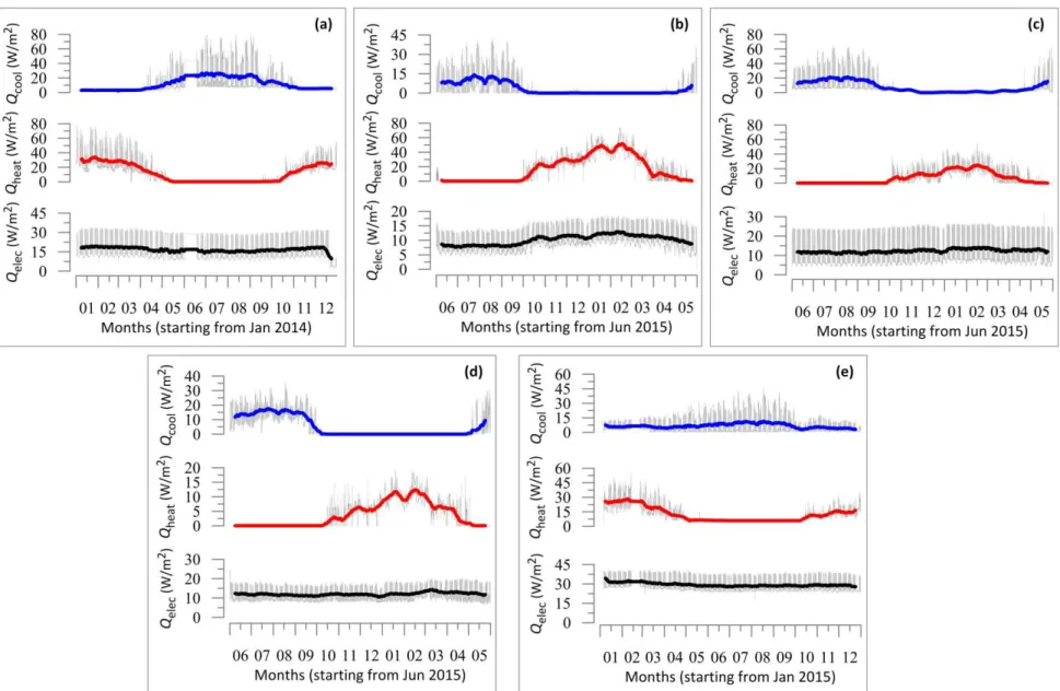
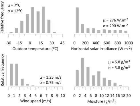
Although the data collection period was between 2013 and 2016, due to interruptions in the data a uisition, only a yea ’s o th of data as e t a ted from each building and used in the model selection part of this study (see Figure 1). Note that although the metered data records for each building were concurrent, they were from different periods for each of the five buildings. However, it was confirmed that the distribution of environmental variables used in modelling each building was nearly identical. Figure 2 presents the distributions of the weather data used in this study. During the observation period, a wide range of weather data was collected (e.g., the outdoor temperatures range
from -30 to 30°C) – which enabled us to study inverse blackbox models under substantially different conditions. As shown in Figure 1, the heating and cooling loads exhibit daily and seasonal variations; whereas electrical loads exhibit only daily variations. It is also worth mentioning that peak heating, cooling, and electrical loads vary substantially from one building to another.
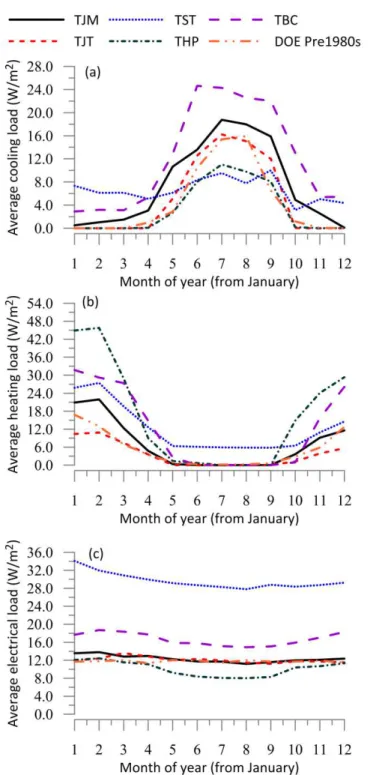
Figure 3 presents the monthly averages for the cooling, heating, and lighting load intensities. The highest of the monthly average heating and cooling load intensities for these buildings were vastly different. In four of the buildings, monthly average cooling load intensities exhibited substantial seasonal variations. As a visual reference while interpreting these values, EnergyPlus simulation results are included in the figure for the archetype pre1980s large office building model [30] using the Canadian Weather Year for Energy Calculation for Ottawa [31]. In three of the four buildings that exhibited seasonal variations, the highest monthly average cooling load was observed in July. In the other one (TBC), the highest monthly average cooling load was observed in June. The cooling loads metered in TBC and TST during the heating seasons and the heating loads metered in TST during the cooling seasons were noticeable. The electrical load intensities did not exhibit a substantial seasonal variation. The minor seasonal variations in the metered electricity usage can be attributed to the seasonal changes in buildings’ o upan y le els e.g., su e a ations) and in the HVAC dist i ution syste s’ e.g., pu ps and fans) efficiency. Recall that the metered electricity usage in the monitored buildings accounts for the energy used by the HVAC distribution systems as well as plug-in equipment and lighting. The average electrical load intensities in the monitored buildings varied by a factor of three, between 10 and 30 W.m
-2
.
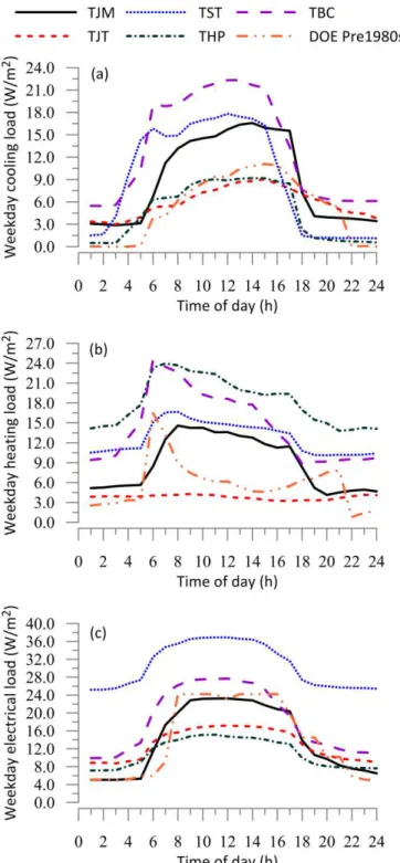
Figure 4 presents the mean weekday heating, cooling, and electrical load intensities of the monitored buildings. Same as Figure 3, the EnergyPlus results for the archetype pre1980s large office building model are included in the figure as a reference. Each plot is prepared by averaging the load measurements recorded at a particular hour on all weekdays. The mean hourly cooling load intensities tend to peak in the afternoons, whereas the mean hourly heating load intensities tend to peak early in the mornings. In one of the monitored buildings (TJT), the mean weekday heating load did not exhibit a diurnal variation. Each building appeared to have a distinct after-hours to work-hours load transition pattern. For example, in TST and TBC, the cooling loads tend to increase to their work-hour values two hours earlier than TJM. In TST and THP, the cooling loads tend to decrease to their after-hours values one hour earlier than TBC and TJM. Simply put, although the data records were collected from the same climatic condition, the diversity in their HVAC equipment, envelope, occupancy, and operation characteristics resulted in substantial variations in their seasonal and diurnal end-use patterns.
3.
Inverse blackbox models
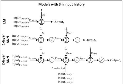
Two different classes of inverse blackbox models were formulated: linear regression models (LM) and artificial neural network (ANN) models. The ANN models were developed at two different complexities: 1-hidden and 1-output layers, and 2-hidden and 1-output layers. After preliminary trials with larger ANN models, we observed that increasing the number of hidden layers further do not improve or decrease the accuracy of the models trained with the datasets of this study. The hidden layers of the ANN models were designed with sigmoid activation functions, whereas the output layers were designed with linear
activation functions. The unknown parameters of the LM models were estimated using the method of least-squares, and the parameters of the ANN models were estimated using the Levenberg-Marquardt backpropagation method [32]. Matla ’s uilt-in function fitlm was used to train the multiple linear eg ession odels. To fo ulate and t ain the ANN odels, Matla ’s uilt-in functions fitnet and train were used. For each model type, the number of inputs of the models was increased incrementally to e eal thei i pa t on the odel’s pe fo an e. The inputs studied in lude the outdoo ai temperature, horizontal solar irradiance, wind speed, moisture content, and metered electrical load intensity. In recognition of the fact that a properly operating office building would have different operating schedules and setpoints outside of nominal work-hours, a work-hour indicator was introduced as a binary categorical variable – attaining the value one between 6 am and 6 pm on weekdays, otherwise zero. A time lag between these inputs and the heating and cooling loads can be expected. For example, current solar irradiance, as it is absorbed by the thermal mass, may affect the heating and cooling loads several hours ahead. This is particularly important for variables that tend to change substantially during the day. For example, for weather data used in this study, the outdoor temperature on average changes about 3°C over a three-hour period. This represents only a small fraction of the total variation in the outdoor temperature. On the other hand, the horizontal solar irradiance on average changes about 200 W/m2 over a three-hour period – which is 76% of the standard deviation of the solar irradiance data record. Thus, the influence of the histo y of odel input alues on the odels’ performance was also studied. Both the ANN and LM models were built so that input values from one-to-three hours before the current time were permitted to affect the heating/cooling loads independently. As a result, 54 inverse blackbox models were built for each of the five buildings at varying number of parameters, inputs, and input histories (i.e., memory). Figure 5 presents a summary of these model forms.
4.
Model selection
Prior to training the models, the relationship between the six model inputs and the heating/cooling loads was investigated. Based on the average of Pearson correlation coefficients computed for each building (see Table 2), a positive correlation exists between the cooling load and outdoor temperature, solar irradiance, and moisture content of air. For the monitored buildings, wind speed appears to be an insignificant factor on the cooling loads. Heating load correlates strongly with the outdoor temperature and moisture content of outdoor air. Wind speed and solar irradiance appear to be secondary factors influencing the heating loads. With increased wind speed, the heating loads tend to increase; and due to an increase in the solar irradiance, the heating loads tend to decrease. Note that there exists a rather unexpected positive correlation between electrical and heating loads. This is likely due to the influence of HVAC distribution loads (e.g., pumps and fans) on the electricity usage. It is also worth noting that some of the model input candidates strongly correlate with each other. For example, because an increase in the outdoor temperature increases the moisture carrying capacity of the outdoor air, a strong positive correlation exists between moisture content of outdoor air and outdoor temperature. In a multiple regression model, this phenomenon is known as multi-collinearity and represents a challenge against training stable and reliable models.
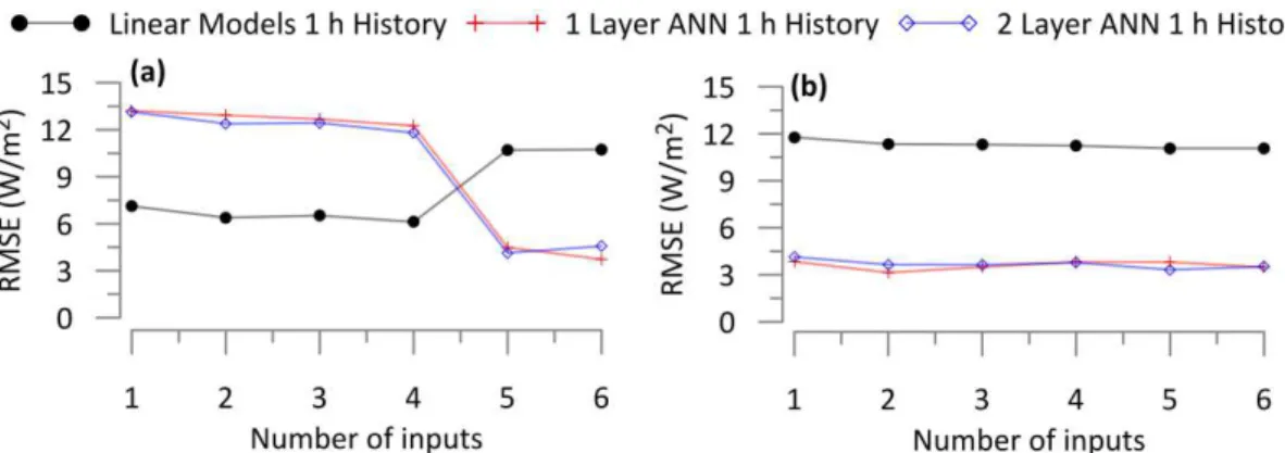
For each building, the models were built by increasing the number of model inputs incrementally in following order: outdoor air temperature, horizontal solar irradiance, wind speed, moisture content of outdoor air, electrical loads, and binary work-hour indicator. Note that considering the collinearity between the outdoor air temperature and the moisture content, we introduced the outdoor air moisture content as the fourth predictor variable after horizontal solar irradiance and wind speed. In other words, because outdoor air temperature and moisture content strongly correlate (the Pearson correlation coefficient is 0.84 in Table 2), using the procedures described in [33], the information that these two variables can provide together was estimated less than it was from the outdoor air temperature and horizontal solar irradiance or the outdoor air temperature and wind speed. Note that the model selection procedure resembles to a forward stepwise regression method – i.e., incrementally increasing the model complexity until satisfactory predictive accuracy can be achieved. However, in lieu of making load forecasts, our purpose in modelling was to characterize the load patterns from various environmental inputs. Because the links between each environmental input and the heating/cooling loads provide unique pieces of information about a building’s ope ation, e intended to in ease the number of inputs after ensuring that the models do not overfit to the test datasets. Three different model structures were studied: LMs, single-layer ANNs, and two-layer ANNs. In each case, a two-fold cross-validation procedure was employed. At each test instance, the data were randomly partitioned into two equal sized groups. Note that the random seed was not constant. Thus, the data used to train and to test the models were different. The models were assessed by looking at the root-mean-square error (RMSE) and R2 values computed upon the validation set (i.e., the portion of the dataset retained for testing purposes). For one of the buildings (TJM), Figure 6 presents the change in the RMSE values with different inputs and model forms. Note that for the LMs, the RMSE values increase (instead of decrease) with the addition of the fifth and sixth inputs. This sign of overfitting did not exist with the ANN models. Results indicate that smaller RMSE values can be achieved with ANNs than LMs. This can e att i uted to ANN’s a ility to ha a te ize non-linearities such as those due to HVAC equipment capacity and performance. However, the difference in the performance of two-layer and one-layer ANNs was marginal for all buildings. This can be interpreted as increasing the number of parameters without increasing the number of inputs available to train an ANN model does not necessarily improve model performance.
The impact of input history was also studied. In other words, the existence of a relationship between current heating/cooling loads and input values one-to-three hours prior to current time was investigated. The history of inputs (i.e., lag variables) used in modelling was incrementally increased as one, two, and three hours. Figure 7 illustrates the impact of using a recent history of input values on the RMSE values of single-layer ANN models for one of the buildings (TJM). The results indicate that using the inputs values two and three hours prior to the current time as complementary predictors did not esult in su stantial i p o e ents in the odels’ p edi ti e a u a y. The ean and standa d de iation of the R2 values (from validation dataset) of models for cooling and heating loads for each model type are summarized in Table 3 and Table 4, respectively. For all five buildings of this study, single-layer ANNs with five inputs and one-hour input history could characterize both the cooling and heating load patterns parsimoniously. Addition of the sixth input (binary work-hours indicator) did not affect the performance of the models. This may be because the electrical loads and binary work-hours indicator
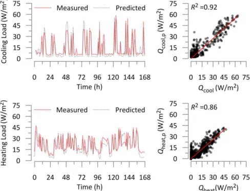
follow a similar trend. However, note that the parameters linking the sixth input and heating/cooling loads could help us understand the impact of after-hours setback or equipment on/off scheduling on the heating and cooling loads. Thus, the selected inverse blackbox model was the one with a single-layer ANN, six inputs and one-hour input history. Figure 8 illustrates the predictive accuracy of the selected model over a representative one-week period (from the validation dataset) for one of the buildings (TJM). The heating and cooling load predictions are made given the input values over this time horizon. In addition, Figure 8 presents the correlation between the predicted and measured heating/cooling load values for the entire validation dataset – not the illustrative one-week period. Visual inspection of these plots indicates that the selected model can represent the overall characteristics of the hourly load (e.g., timing and magnitude of the local extrema) at a reasonable accuracy.
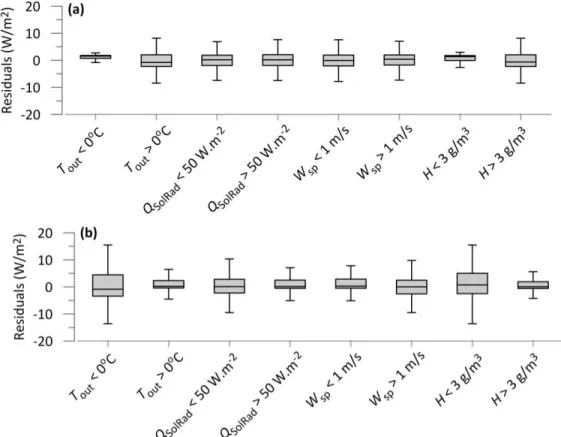
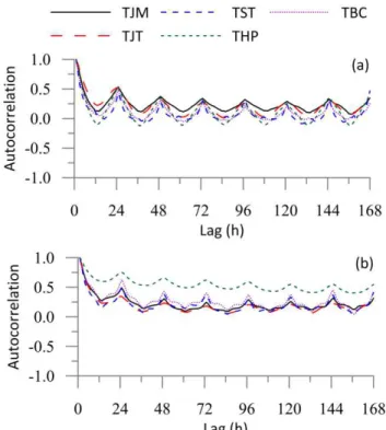
The appropriateness of the selected model was further investigated through a residual analysis. The residuals are the differences between observed and estimated heating/cooling load values. Each data point – at hourly intervals – has one residual. If the selected model is appropriate, the sums of residuals should add up to zero under all types of input levels – i.e., predictions show no systematic negative/positive bias. Figure 9.a and b present the distribution of the residuals under different environmental conditions for cooling and heating loads, respectively. By visual inspection, the results indicate that the mean of the residuals remains unchanged at zero under different conditions. However, the variance of residuals changes substantially – particularly with moisture content and temperature of outdoor air. This is expected because the variance of residuals should change proportional to the dependent variable (i.e., heating and cooling loads). The autocorrelation of residuals is shown in Figure 10. These autocorrelation plots illustrate how well the residual time-series would correlate to itself if it is shifted by a time-lag. Ideally, the residual autocorrelation of a model should resemble to that of a white-noise, so that the modelling error does not exhibit any periodicity. The diurnal periodicity and the weak autocorrelation extending beyond 24 h underline that the selected model does not meet this residual whiteness criterion. This should be acknowledged as a limitation of the studied approach, and it may detrimentally affect our ability to make controls and operational interventions quickly.
5.
Discussion on use cases of inverse blackbox models
Because the selected model (single-layer ANN) links the input values to the dependent variables in a non-linear fashion, it is challenging to interpret the parameter estimates. Thus, in lieu of interpreting parameter estimates directly, the partial derivatives of the dependent variables with respect to input variables were calculated – e.g., the rate of change in the heating load intensity with outdoor temperature (dQheat/dTout), the rate of change in the cooling load intensity with outdoor air moisture
content (dQcool/dH), and so on. While calculating the partial derivatives, the parameters other than the
two used in a particular partial derivative held constant. It was assumed that the outdoor temperature is -10°C for winter and 20°C for summer, outdoor air moisture content is 1 g/m3 for winter and 15 g/m3 for summer, solar irradiance is 100 W/m2, wind speed is 1 m/s, and electrical load intensity is 10 W/m2. Appropriateness of these assumptions was verified through a sensitivity study. In a similar fashion, an EnergPlus simulation was conducted using the pre1980s large office building archetype model [30] and a standard weather year for Ottawa, Canada [31]. Hourly heating, cooling, and electrical load intensities were extracted from the simulation results, and analyzed with concurrent weather data. Aside from the
data gathered from the five buildings, the selected model (single-layer ANN) was trained with this synthetic dataset, and partial derivative values were calculated. The purpose of this exercise is to generate a reference case for the five buildings of this study. Modelling details and assumptions related with the archetype energy models can be found elsewhere [30].
Table 5 and Table 6 present these partial derivatives for the cooling and heating load intensities, respectively. Note that each model input affects the heating and cooling load intensities for each building in a different way. For example, the heating and cooling load intensities in THP are substantially affe ted y the hanges in outdoo te pe atu e; he eas these hanges play a inis ule ole fo TST’s heating and cooling loads. Note that these partial derivatives can be used in building operation. Herein, two use cases are briefly discussed: (1) establishing performance benchmarks across a building cluster, and dete ting issues in a uilding’s syste s and o ponents. Note that these appli ations an help facility managers decide how available resources are allocated for retrofits and maintenance.
Table 7 illustrates the relationship between several performance indicators for building envelope and equipment and these partial derivatives. For example, high ��� �
�� and ��ℎ��
�� values can be an indication
of low thermal insulation or a leaky envelope. Another reason for high ��� �
�� and ��ℎ��
�� can be poorly
sized and controlled HVAC equipment (e.g., high outdoor airflow fraction at the air-handling unit, inappropriate economizer and heat recovery programs). Similarly, high ��� �
�� and ��ℎ��
�� can be an
indication of relatively high air-permeability (e.g., air-barrier failures). If the outdoor air fraction is too high (e.g., outdoor air damper stuck open), the role of outdoor moisture content on the heating load intensity ��ℎ��
�� will increase. For an office building with standard occupancy, if the effect of binary
work-hours indicatoron the heating or cooling load intensities ��� �,ℎ��
���ℎ is nearly-zero or positive, this
is an indication of ineffective after-hours scheduling. This may happen due to manual overrides to the AHU schedules or faulty fan/pump actuators that continue to operate in the evenings and weekends. Therefore, comparison of the partial derivative values across a building cluster can help us identify some of the weaknesses of each building; and their variations in time can help us detect some of the faults in
uildings’ syste s and o ponents. When we compare ��ℎ��
�� and ��ℎ��
�� values, it appears that heating and cooling energy intensity of THP
depends heavily on the envelope losses and thus it might be a good candidate for envelope improvements that reduce thermal, air, vapour leakage to outdoors during the heating season. The independent building audits conducted in THP in 2009 also identified substantial envelope issues such as drafts near exterior window and walls. When the ��ℎ��
���ℎ values are compared, after-hours and weekend
heating load patterns in TST, TJM, and TJT appeared similar to those observed during work-hours. This can be interpreted that after-hours HVAC equipment scheduling was ineffective. In line with this interpretation, recent building audits conducted in TJT identified that the AHUs serving perimeter heating induction units were not scheduled. Similarly, the audits conducted in TJM identified that twelve of the fourteen AHUs operate from 6 am to midnight including weekends and holidays.
Note that the purpose of this paper is to put forward the idea of inverse blackbox modelling to characterize heating and cooling load patterns in cases where no or limited sensor data are available for greybox modelling. Herein, we demonstrated a few examples in which such models can find application to support operational decision making process. Although these preliminary results and discussion are promising, there are several unresolved issues left for future work:
1) Use of in e se la k o odelling to ha a te ize a uilding’s ene gy pe fo an e has een demonstrated using the metered data from five large office buildings. Future work is planned to expand the analyses to a larger number of buildings from different vintages.
2) Inverse blackbox models can help us detect system or plant level issues that substantially affect the heating and cooling load patterns of a building. However, they cannot isolate and diagnose these improper operating conditions. Therefore, they are complementary – not an alternative – to fault detection and diagnostics methods that incorporate the indoor sensing functionalities of modern automation and control networks.
3) The inverse blackbox models can be trained using batch data at regular intervals (e.g., once every six months). As discussed earlier, the deviations in partial derivatives in time can help us reveal developing issues in the envelope or HVAC equipment operation; and comparisons across a building cluster can help us establish a performance baseline. However, we need to better understand and quantify the uncertainty in these partial derivatives, so that their evolution in time can be correctly interpreted. Future work should also study the stochasticity of inverse blackbox models using a larger dataset from more buildings.
6.
Conclusions
Using heating, cooling, and electrical load data gathered in five office buildings, this paper put forward a systematic method to select an inverse blackbox model that can characterize the heating and cooling load patterns parsimoniously. To this end, 18 different forms of model at varying numbers of inputs and pa a ete s e e e a ined fo ea h of the fi e uildings. The odels’ pe fo an e as assessed through a two-fold cross-validation and a residual analysis. In line with the recent findings reported in the literature, artificial neural network models appeared to perform better than linear regression models in characterizing the heating and cooling load patterns. However, increasing the complexity of artificial neural network models beyond 1-hidden and 1-output layers did not result in any notable i p o e ents in the odels’ pe fo an e. It as o se ed that in easing the nu e of pa a ete s used in fitting the model without increasing the number of model inputs reduced, instead of increased, the odel’s p edi ti e a u a y. Diffe ent inputs e e studied: outdoo ai te pe atu e, horizontal solar irradiance, (3) wind speed, (4) moisture content of the outdoor air, (5) electrical load intensity, and (6) a binary work-hours indicator (one from 6 am to 6 pm on weekdays and zero otherwise). In an effort to mimic the transient nature of heat transfer and storage inside buildings, the effect of input history was studied such that the input values one to three hours prior to current time were permitted to affect current heating and cooling loads. It was found that a one-hour history was adequate for the studied buildings for both heating and cooling loads. Upon these data analyses, a model was selected. The selected model is the one with one-layer ANN with six inputs and one-hour input history.
Different use cases for these models were discussed. Two of these use-cases were (1) establishing a performance benchmark across a building cluster by comparing the model parameters from different buildings and (2) detecting envelope and equipment issues by looking at the changes in model parameters in time. Based on a few illustrative examples, the potential of inverse blackbox modelling in operational decision making was demonstrated. Future work should investigate the use of these models in detecting improper operating conditions using comprehensive fault-symptom datasets and data from a larger number of buildings.
Acknowledgements
The work presented in this paper was supported by the Smart Building Project (A1-006050) administered by Public Services and Procurement Canada (PSPC).
References
1. NRCan, Energy use data handbook 1990 to 2010, 2013, National Resources Canada. 2. DOE, Buildings energy data book, 2011, United States Department of Energy.
3. CABA, Intelligent buildings and big data, 2015, Continental Automated Buildings Association: Ottawa.
4. Yik, F.W.H., Burnett, J. and Prescott, I., 2001. Predicting air-conditioning energy consumption of a group of buildings using different heat rejection methods. Energy and Buildings, 33(2), pp.151-166.
5. Pan, Y., Huang, Z. and Wu, G., 2007. Calibrated building energy simulation and its application in a high-rise commercial building in Shanghai. Energy and Buildings, 39(6), pp.651-657.
6. Zhou, Q., Wang, S., Xu, X. and Xiao, F., 2008. A grey‐box model of next‐day building thermal load prediction for energy‐efficient control. International Journal of Energy Research, 32(15), pp.1418-1431.
7. Braun, J.E. and Chaturvedi, N., 2002. An inverse gray-box model for transient building load prediction. HVAC&R Research, 8(1), pp.73-99.
8. Wang, S. and Xu, X., 2006. Simplified building model for transient thermal performance estimation using GA-based parameter identification. International Journal of Thermal
Sciences, 45(4), pp.419-432.
9. Hou, Z., Lian, Z., Yao, Y. and Yuan, X., 2006. Cooling load prediction based on the combination of rough set theory and support vector machine. HVAC&R Research, 12(2), pp.337-352.
10. Kusiak, A., Li, M. and Zhang, Z., 2010. A data-driven approach for steam load prediction in buildings. Applied Energy, 87(3), pp.925-933.
11. Dong, B., Cao, C. and Lee, S.E., 2005. Applying support vector machines to predict building energy consumption in tropical region. Energy and Buildings, 37(5), pp.545-553.
12. Yang, J., Rivard, H. and Zmeureanu, R., 2005. On-line building energy prediction using adaptive artificial neural networks. Energy and buildings, 37(12), pp.1250-1259.
13. Newsham, G.R. and Birt, B.J., 2010, November. Building-level occupancy data to improve ARIMA-based electricity use forecasts. In Proceedings of the 2nd ACM workshop on embedded
sensing systems for energy-efficiency in building (pp. 13-18). ACM.
14. Chokor, A. and El Asmar, M., 2016. Data-Driven Approach to Investigate the Energy Consumption of LEED-Certified Research Buildings in Climate Zone 2B. Journal of Energy
Engineering, p.05016006.
15. Li, Q., Meng, Q., Cai, J., Yoshino, H. and Mochida, A., 2009. Applying support vector machine to predict hourly cooling load in the building. Applied Energy, 86(10), pp.2249-2256.
16. Li, Q., Meng, Q., Cai, J., Yoshino, H. and Mochida, A., 2009. Predicting hourly cooling load in the building: a comparison of support vector machine and different artificial neural networks. Energy Conversion and Management, 50(1), pp.90-96.
17. Kwok, S.S. and Lee, E.W., 2011. A study of the importance of occupancy to building cooling load in prediction by intelligent approach. Energy Conversion and Management, 52(7), pp.2555-2564.
18. Kapetanakis, D., Mangina, E., Ridouane E., Kouramas K. and Finn, D., 2015. Comparison of predictive models for forecasting building heating loads, Building Simulation Conference, IBPSA: India.
19. Kapetanakis, D.S., Mangina, E. and Finn, D., 2015. Methodology for commercial buildings thermal loads predictive models based on simulation performance. International Conference on
Simulation Tools and Techniques, ICST: Greece.
20. Jo ano ić, R.Ž., S eteno ić, A.A. and Ži ko ić, B.D., 2015. Ensemble of various neural networks
for prediction of heating energy consumption. Energy and Buildings, 94, pp.189-199.
21. Sun, Y., Wang, S. and Xiao, F., 2013. Development and validation of a simplified online cooling load prediction strategy for a super high-rise building in Hong Kong. Energy Conversion and
Management, 68, pp.20-27.
22. Taylor, J.W., 2012. Short-term load forecasting with exponentially weighted methods. IEEE
Transactions on Power Systems, 27(1), pp.458-464.
23. Gunay, H.B., O’B ien, W. and Beausoleil-Morrison, I., 2016. Control-oriented inverse modeling of
the thermal characteristics in an office. Science and Technology for the Built Environment, pp.1-20.
24. Bacher, P. and Madsen, H., 2011. Identifying suitable models for the heat dynamics of buildings. Energy and Buildings, 43(7), pp.1511-1522.
25. Lazos, D., Sproul, A.B. and Kay, M., 2014. Optimisation of energy management in commercial buildings with weather forecasting inputs: A review. Renewable and Sustainable Energy
Reviews, 39, pp.587-603.
26. Zixiao, S., O'Brien, W. and Gunay, H.B., 2016. Building zone fault detection with Kalman filter-based methods, eSim Conference, IBPSA Canada: Hamilton, Ontario.
27. Usoro, P.B., Schick, I.C. and Negahdaripour, S., 1985. An innovation-based methodology for HVAC system fault detection. Journal of dynamic systems, measurement, and control, 107(4), pp.284-289.
28. Gunay, H.B., O'Brien, W., Beausoleil-Morrison, I., Bisaillon, P. and Shi, Z., 2016. Development and implementation of control-oriented models for terminal heating and cooling units. Energy
and Buildings, 121, pp.78-91.
29. Mulumba, T., Afshari, A. and Friedrich, L., 2014. Kalman filter-based Fault Detection and Diagnosis for Air Handling Units. International Refrigeration and Air Conditioning Conference, Purdue University: Indiana.
30. Deru, M., Field, K., Studer, D., Benne, K., Griffith, B., Torcellini, P., Liu, B., Halverson, M., Winiarski, D., Rosenberg, M. and Yazdanian, M., 2011. US Department of Energy commercial reference building models of the national building stock.
31. Environment Canada, 2016. Engineering Climate Datasets, Government of Canada, Ottawa, Ontario.
32. Wythoff, B.J., 1993. Backpropagation neural networks: a tutorial. Chemometrics and Intelligent
Laboratory Systems, 18(2), pp.115-155.
33. May, R., Dandy, G. and Maier, H., 2011. Review of input variable selection methods for artificial
List of Figures:
Figure 1: Data records for cooling (Qcool), heating (Qheat), and electrical (Qelec) load intensities for (a) TBC,
(b) THP, (c) TJM, (d) TJT, and (e) TST. Solid lines represent the mean running average over a 15-day period.
Figure 2: Environmental conditions during the data collection period (for the entire three years).
Figure 3: Monthly averages for the (a) cooling, (b) heating, and (c) electrical load intensities in the five
monitored buildings. EnergyPlus results from the archetype large pre1980s office building model [30] are included as a reference.
Figure 4: Mean weekday (a) cooling, (b) heating, and (c) electrical load intensities in the five monitored
buildings. EnergyPlus results from the archetype large pre1980s office building model [30] are included as a reference.
Figure 5: The inverse blackbox models at varying number of parameters, inputs, and input histories. Figure 6: The effect of model structure and complexity on the root-mean-square error (RMSE) of the
odels’ offline p edi tions fo a ooling and heating loads. Fo illust ati e pu poses, only the esults from TJM were used.
Figure 7: The effect of input history on the root-mean-square error (RMSE) of the models’ offline
predictions for (a) cooling and (b) heating loads. For illustrative purposes, only the results from TJM were used.
Figure 8: Line plots illust ate the sele ted odel’s pe fo an e o e a ep esentati e eek of one of the
buildings (TJM). Scatter plots illustrate the deviation between the predicted (Qheat,p andQcool,p) and the
measured (Qheat andQcool) heating/cooling loads.
Figure 9: Dist i ution of the sele ted odels’ esiduals unde diffe ent en i on ental onditions fo a
cooling and (b) heating loads. Tout, QSolRad, Wsp, H are the outdoor temperature (°C), horizontal solar
irradiance (W.m-2), wind speed (Wsp), and moisture content of the outdoor air (g/m 3
), respectively.
Figure 1: Data records for cooling (Qcool), heating (Qheat), and electrical (Qelec) load intensities for (a) TBC, (b) THP, (c) TJM, (d) TJT, and (e) TST.
Figure 3: Monthly averages for the (a) cooling, (b) heating, and (c) electrical load intensities in the five
monitored buildings. EnergyPlus results from the archetype large pre1980s office building model [30] are included as a reference.
Figure 4: Mean weekday (a) cooling, (b) heating, and (c) electrical load intensities in the five monitored
buildings. EnergyPlus results from the archetype large pre1980s office building model [30] are included as a reference.
Figure 6: The effect of model structure and complexity on the root-mean-square error (RMSE) of the
odels’ offline p edi tions fo a ooling and heating loads. Fo illust ati e pu poses, only the esults from TJM were used.
Figure 7: The effect of input history on the root-mean-s ua e e o RMSE of the odels’ offline
predictions for (a) cooling and (b) heating loads. For illustrative purposes, only the results from TJM were used.
Figure 8: Line plots illust ate the sele ted odel’s pe fo an e o e a ep esentati e eek of one of the
buildings (TJM). Scatter plots illustrate the deviation between the predicted (Qheat,p andQcool,p) and the
Figure 9: Dist i ution of the sele ted odels’ esiduals unde diffe ent en i on ental onditions fo a
cooling and (b) heating loads. Tout, QSolRad, Wsp, H are the outdoor temperature (°C), horizontal solar
irradiance (W.m-2), wind speed (Wsp), and moisture content of the outdoor air (g/m 3
Tables
Table 1: Overview of the monitored buildings.
Table 2: Average of the Pearson correlation coefficients calculated for the five buildings. Negative values
less than -0.05 are in bold and italicised (red) font, and positive values more than 0.05 are in bold (blue) font.
Table 3: The mean and standard deviation of the R2 values for the inverse blackbox models predicting the uildings’ ooling loads. The R2
values were computed for each of the 18 models by using a portion of the dataset retained for validation. The R2 values were calculated for each of the five buildings separately, and then their means and standard deviations are reported in the table.
Table 4: The mean and standard deviation of the R2 values for the inverse blackbox models predicting the uildings’ heating loads. The R2
values were computed for each of the 18 models by using a portion of the dataset retained for validation. The R2 values were calculated for each of the five buildings separately, and then their means and standard deviations are reported in the table.
Table 5: The rate of change in the cooling load Qcool (W/m 2
) with respect to the model inputs: outdoor air temperature Tout (°C), horizontal solar irradiance QSolRad (W/m
2
), wind speed Wsp (m/s 2
), moisture content of outdoor air H(g/m3), electrical loads Qelec (W/m
2
), binary work-hours indicator Bwh.
Table 6: The rate of change in the heating load Qheat (W/m 2
) with respect to the model inputs: outdoor air temperature Tout (°C), horizontal solar irradiance QSolRad (W/m
2
), wind speed Wsp (m/s 2
), moisture content of outdoor air H(g/m3), electrical loads Qelec (W/m
2
), binary work-hours indicator Bwh.
Table 7: Illustrative examples to improper operating conditions, and their relationships with the partial
Table 1: Overview of the monitored buildings.
Building Floor Area (m2) Vintage Primary Equipment Secondary Equipment
TBC 28889 1965 VAV AHUs scheduled 5 am to 9 pm weekdays 8 am to 5 pm weekends
Perimeter induction VAV terminal units
THP 12432 1956 CAV and VAV AHUs No schedule
Hydronic radiant heaters VAV terminal units TJM 38430 1970 CAV AHUs scheduled
6 am to 12 am weekdays and weekends
Perimeter induction CAV terminal units
TJT 70970 1979 VAV AHUs scheduled 5 am to 6 pm weekdays (schedule is overridden during heating season)
Perimeter induction VAV terminal units
TST 45123 1952 VAV and CAV scheduled 6 am to 5 pm weekdays only
Perimeter induction CAV terminal units
Table 2: Average of the Pearson correlation coefficients calculated for the five buildings. Negative values
less than -0.05 are in bold and italicised (red) font, and positive values more than 0.05 are in bold (blue) font. Variables Cooling Load Heating Load Outdoor Temperature Solar Irradiance Wind Speed Moisture Content Electrical Load Cooling Load 1.00 -0.32 0.49 0.28 -0.02 0.54 0.39 Heating Load 1.00 -0.83 -0.08 0.11 -0.65 0.36 Outdoor Temperature 1.00 0.23 -0.04 0.84 -0.16 Solar Irradiance 1.00 0.28 -0.01 0.30 Wind Speed 1.00 -0.15 0.13 Moisture Content 1.00 -0.14 Electrical Load 1.00
Table 3: The mean and standard deviation of the R2 values for the inverse blackbox models predicting the uildings’ ooling loads. The R2
values were computed for each of the 18 models by using a portion of the dataset retained for validation. The R2 values were calculated for each of the five buildings separately, and then their means and standard deviations are reported in the table.
Number
of inputs History (h)
Linear Models 1 Layer ANN 2 Layer ANN Mean Std Mean Std Mean Std 1 1 0.09 0.06 0.30 0.24 0.27 0.23 2 1 0.12 0.07 0.33 0.20 0.34 0.22 3 1 0.12 0.07 0.33 0.21 0.34 0.19 4 1 0.12 0.09 0.38 0.21 0.45 0.17 5 1 0.28 0.29 0.87 0.03 0.89 0.03 6 1 0.28 0.29 0.88 0.03 0.87 0.03 1 2 0.13 0.08 0.38 0.18 0.41 0.20 2 2 0.14 0.09 0.42 0.17 0.44 0.18 3 2 0.14 0.09 0.39 0.19 0.43 0.19 4 2 0.15 0.11 0.44 0.19 0.47 0.15 5 2 0.29 0.29 0.88 0.02 0.89 0.03 6 2 0.29 0.29 0.87 0.04 0.91 0.03 1 3 0.14 0.08 0.40 0.19 0.40 0.20 2 3 0.14 0.10 0.39 0.22 0.46 0.18 3 3 0.15 0.10 0.43 0.16 0.45 0.17 4 3 0.15 0.12 0.47 0.16 0.47 0.19 5 3 0.29 0.29 0.87 0.05 0.90 0.01 6 3 0.29 0.29 0.88 0.02 0.89 0.03
Table 4: The mean and standard deviation of the R2 values for the inverse blackbox models predicting the uildings’ heating loads. The R2
values were computed for each of the 18 models by using a portion of the dataset retained for validation. The R2 values were calculated for each of the five buildings separately, and then their means and standard deviations are reported in the table.
Number
of inputs History (h)
Linear Models 1 Layer ANN 2 Layer ANN Mean Std Mean Std Mean Std 1 1 0.61 0.14 0.63 0.15 0.64 0.15 2 1 0.61 0.13 0.64 0.15 0.63 0.16 3 1 0.61 0.13 0.65 0.14 0.63 0.17 4 1 0.61 0.12 0.64 0.13 0.67 0.12 5 1 0.62 0.09 0.73 0.19 0.77 0.16 6 1 0.62 0.09 0.72 0.20 0.75 0.18 1 2 0.62 0.13 0.70 0.22 0.66 0.15 2 2 0.61 0.12 0.63 0.16 0.65 0.16 3 2 0.61 0.12 0.63 0.15 0.65 0.17 4 2 0.61 0.12 0.67 0.15 0.64 0.15 5 2 0.62 0.09 0.75 0.18 0.79 0.15 6 2 0.62 0.08 0.63 0.31 0.77 0.22 1 3 0.62 0.12 0.65 0.15 0.66 0.15 2 3 0.61 0.12 0.65 0.15 0.66 0.15 3 3 0.61 0.12 0.67 0.15 0.67 0.16 4 3 0.61 0.12 0.66 0.13 0.67 0.11 5 3 0.62 0.09 0.74 0.21 0.77 0.18 6 3 0.62 0.08 0.79 0.14 0.80 0.16
Table 5: The rate of change in the cooling load Qcool (W/m 2
) with respect to the model inputs: outdoor air temperature Tout (°C), horizontal solar irradiance QSolRad (W/m
2
), wind speed Wsp (m/s 2
), moisture content of outdoor air H(g/m3), electrical loads Qelec (W/m
2
), binary work-hours indicator Bwh.
Buildings � � � � � � � � � � ���� TJM 1.3 0.001 -3.5 0.81 1.67 -2.7 TJT 0.9 0.001 -1.2 0.76 0.65 0.1 TBC 0.7 0.000 -1.1 0.42 0.97 -3.9 THP 1.8 0.002 -3.3 1.60 4.00 1.1 TST-2015 0.0 0.000 0.0 0.03 0.05 -0.1 TST-2016 0.0 0.000 0.0 0.02 0.04 -0.1 DOE pre1980s 2.7 0.001 -0.3 2.28 1.45 -2.2
Table 6: The rate of change in the heating load Qheat (W/m 2
) with respect to the model inputs: outdoor air temperature Tout (°C), horizontal solar irradiance QSolRad (W/m
2
), wind speed Wsp (m/s 2
), moisture content of outdoor air H(g/m3), electrical loads Qelec (W/m
2
), binary work-hours indicator Bwh.
Buildings � � � � � � � � � � �� � �� �� ��� TJM -1.0 -0.005 0.6 -0.44 0.73 0.2 TJT -0.7 0.000 0.4 0.17 0.08 -0.3 TBC -0.6 -0.006 0.8 -1.92 0.71 -1.4 THP -1.8 -0.004 1.1 0.31 1.84 -2.9 TST-2015 -0.1 -0.001 0.2 -0.28 0.19 0.2 TST-2016 -0.1 -0.001 0.2 -0.23 0.17 0.1 DOE pre1980s -0.9 -0.003 0.3 0.52 0.10 0.1
Table 7: Illustrative examples to improper operating conditions, and their relationships with the partial
derivatives of heating/cooling loads with respect to model inputs.
��� � �� ��ℎ�� �� ��� � �� ��ℎ�� �� ����� � ��ℎ�� �� ��� � ���ℎ ��ℎ�� ���ℎ
Potential Operational Issues
↑ ↑ — — — — — — Thermal insulation degradation
↑ ↑ ↑ ↑ — — — — High air-permeability
— — — — — ↑ — — High vapour-permeability
↓ ↓ — — — ↓ — — Low outdoor air fraction in ventilation (e.g., damper stuck closed)
↑ ↑ — — — ↑ — — High outdoor air fraction in ventilation (e.g., damper stuck open)
↓ ↑ — — — — — — High AHU supply temperature (e.g., faulty sensor, faulty heating/cooling coil valve)
↑ ↓ — — — — — — Low AHU supply temperature (e.g., faulty sensor, faulty heating/cooling coil valve)
— — — — ↓ ↑ — — High AHU supply humidity (e.g., faulty sensor, faulty humidifier valve)
— — — — ↑ ↓ — — Low AHU supply humidity (e.g., faulty sensor, faulty humidifier valve)
— — — — — — — ↓ Ineffective after-hours schedule for heating (e.g., manual overrides, issues in pumps, fans)