Analysis and design of propulsive guidance for atmospheric skip entry trajectories

Analysis and Design of Propulsive Guidance for

Atmospheric Skip Entry Trajectories

by

Garrett Oliver Teahan

B.S., Aeronautical and Astronautical Engineering University of Washington (2004)

Submitted to the Department of Aeronautics and Astronautics in partial fulfillment of the requirements for the degree of

Master of Science in Aeronautics and Astronautics at the

MASSACHUSETTS INSTITUTE OF TECHNOLOGY May 2006

@

Garrett Oliver Teahan, MMVI. All rights reserved.

The author hereby grants to MIT permission to reproduce and distribute publicly paper and electronic copies of this thesis document in whole or in part.

(I1 s .'

ARMES

7MASSACHUSETTSINSTUTE OF TECHNOLOGY

JUN 2 3 2010

LIBRARIES Author:

Department of Aeronautics and Astronautics May 26, 2006 Certified by: The Charles Certified by: -Senior Lectu r in Stephen C. Paschall II Member of Technical Staff Stark Draper Laboratory, Inc. Technical Supervisor Richard H. Battin, Ph.D. Aeronautics and Astronautics Thesis Advisor Accepted by:

Jaime Peraire Professor of Aeronautics and Astronautics Chair, Committee on Graduate Students

Analysis and Design of Propulsive Guidance for Atmospheric

Skip Entry Trajectories

by

Garrett Oliver Teahan

Submitted to the Department of Aeronautics and Astronautics on May 26, 2006, in partial fulfillment of the

requirements for the degree of

Master of Science in Aeronautics and Astronautics

Abstract

A study of the ability to use propulsive guidance for atmospheric skip entry trajec-tories was completed. The analysis centered itself around the proposed design of NASA's Crew Exploration Vehicle. The primary aerodynamic guidance system must execute an atmospheric skip maneuver when attempting to reach distant landing sites. These maneuvers result in the loss of aerodynamic control authority during the skip phase. The physics of the problem were studied through an analysis of the minimum impulsive AV. This analysis was completed for a number of different tra-jectories with varying energies. The framework of the propulsive guidance algorithm, derived from the Powered Explicit Guidance law of the Space Shuttle, was presented and the augmented design was explained. The sensitivity of the propulsive guidance solution to a given trajectory was explored as well as its response to altitude con-strained maneuverability. The robustness of the algorithm is measured using Monte Carlo techniques. The results showed that the current design of the Crew Explo-ration Vehicle and the current implementation of the primary aerodynamic guidance system are inadequate for a precise, long range, crewed return from the Moon. It was also shown that the lower energy trajectories are more favorable given the altitude reorientation constraint. It was recommended that the skip phase be redefined such that it does not begin until the altitude reorientation constraint is met. It was shown that a combination of increasing the total amount of thrust available, AV allowance, and the entry guidance precision are necessary to bring the success rate to acceptable levels for a precise, long range, crewed return from the Moon.

Technical Supervisor: Stephen C. Paschall II Title: Member of Technical Staff

The Charles Stark Draper Laboratory, Inc. Thesis Advisor: Richard H. Battin, Ph.D.

Acknowledgments

There are a number of people without which this thesis would not have been com-pleted. I would like to thank my technical supervisor, Steve Paschall. His insight and understanding were invaluable. It has been great working with him and I would hope it will be possible to work with him again in the future. I would also like to thank Gregg Barton, Sarah Bairstow, Roberto Pileggi, and Sungyung Lim whose work has led to the problem discussed in this thesis. Sean George was very helpful in understanding the aerodynamics of capsules in rarefied flow. Peter Neirinckx was my advisor during the early part of my graduate studies and his guidance was rewarding. Brooke Marquardt and the library staff were great at helping me dig up old refer-ences about the Soviet space program. I would also like to thank George Schmidt and The Charles Stark Draper Laboratory for giving me the opportunity to study at the Massachusetts Institute of Technology while working with some of top engineers in this field.

I would also like to show my appreciation to Zach Putnum, Melanie Miller, and Geoff Huntington (the officemate that never was) for sharing an office with me and keeping me entertained when I needed it most. I would also like to thank the Friday Morning Donuts Crew for allowing to me consume more than my fair share of the dozen.

My greatest thanks is given to my family whose love, support, and encouragement has made me who I am today. I'm looking forward to finally joining the rest of you in the real world. I would especially like to thank my mother for having the courage and patience to raise me from my day one to day 8943. You've always been there for me ever since my first days in that tiny loft in San Francisco and I can't thank you enough.

This thesis was prepared at The Charles Stark Draper Laboratory, Inc., under Inter-nal Research and Development, Project GCDLF-Support, 20340:001.

Publication of this thesis does not constitute approval by Draper or the sponsor-ing agency of the findsponsor-ings or conclusions contained herein. It is published for the exchange and stimulation of ideas.

Contents

1 Introduction 1.1 Presidential Vision . . . . 1.2 Background . . . . 1.3 Motivation... . . . . . . . . . 1.4 Objective . . . . 1.5 Overview . . . . 2 Simulation Environment 2.1 Coordinate Frames . . . . 2.1.1 Earth-centered . . . . 2.1.2 Spacecraft-centered . . . . . 2.1.3 Coordinate Transformations 2.2 Environment Model . . . . ... 2.2.1 Atmosphere Model . . . . . 2.2.2 Gravity Model . . . . 2.3 Vehicle Model . . . . 2.4 Equations of Motion . . . . 2.5 Boundary Conditions . . . . 3 Impulsive Analysis 3.1 Trajectory Classification . . . . 3.2 Aerodynamic Effects . . . . 3.3 Downrange Targeting . . . . 31 32 32 33 35 37 38 38 39 41 43 49 50 52 53 . . . . . . . . . . . .

3.4 Correction Capability . . . . 62

3.5 Manifold Targeting . . . . 67

4 Guidance Design 77 4.1 Powered Explicit Guidance . . . . 78

4.1.1 Guidance Equations . . . . 78

4.1.2 Linear Terminal Velocity Constraint . . . . 81

4.2 Augmented Algorithm . . . . 83

5 Results 87 5.1 Trajectory Sensitivity . . . . 87

5.2 Environment, Vehicle, and State Uncertainties . . . . 96

5.3 Monte Carlo Results . . . . 98

6 Conclusion 115 6.1 Summary . . . . 115

6.2 Future Work . . . . 116

A Impulsive AV Direction 119 A.1 Downrange Targeting . . . . 119

A.2 Manifold Targeting . . . . 122

B Dispersed Variables 125 B.1 Required AV Magnitude . . . . 125

B.1.1 Atmospheric Density... . . . .. 125

B.1.2 Spacecraft Mass . . . . 128

B.1.3 Spacecraft Lift Coefficient . . . . 131

B.1.4 Spacecraft Drag Coefficient . . . . 134

B.1.5 Thruster Force . . . . 137

B.1.6 Initial Velocity . . . . 140

B.2 Residual Manifold Targeting Error . . . . 143

Spacecraft Mass . . . . Spacecraft Lift Coefficient Spacecraft Drag Coefficient Thruster Force . . . . Initial Velocity . . . . B.2.2 B.2.3 B.2.4 B.2.5 B.2.6 146 149 152 155 158 . . . . . . . . . . . . . . . . . . . .

List of Figures

1-1 An example of an atmospheric skip entry trajectory . . . . 23

1-2 Effective regimes for aerodynamic and propulsive guidance . . . . 27

2-1 Earth-centered coordinate frames . . . . 33

2-2 Spacecraft-centered coordinate frames . . . . 35

2-3 CEV shape . . . . 40

2-4 Propulsive guidance range corrections . . . . 46

3-1 Nominal skip trajectories . . . . 51

3-2 Range control authority of lift during the skip phase . . . . 53

3-3 Impulsive AV at the initiation of the skip phase . . . . 56

3-3 Impulsive AV at the initiation of the skip phase (cont'd) . . . . 57

3-3 Impulsive AV at the initiation of the skip phase (cont'd) . . . . 58

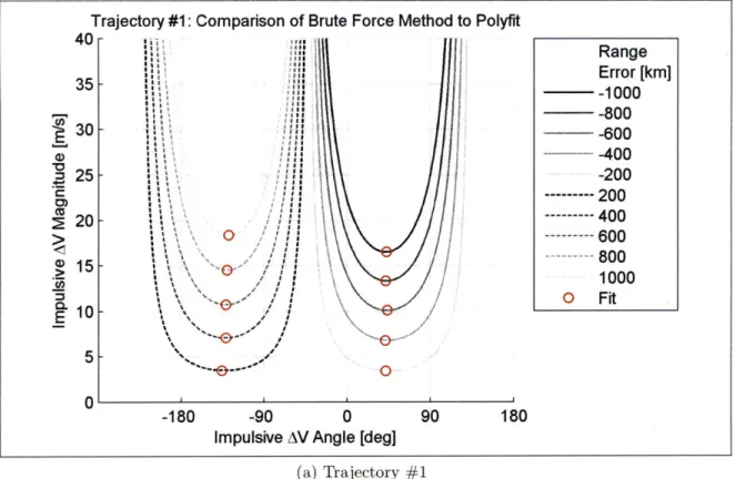
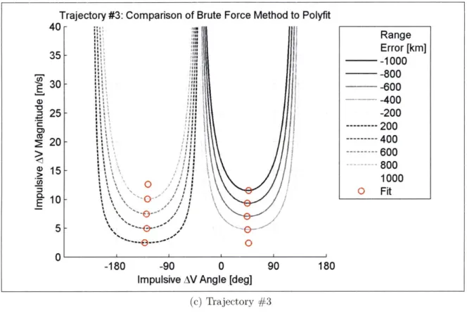
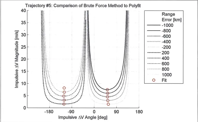
3-4 Minimum impulsive AV to target a downrange location . . . . 60

3-4 Minimum impulsive AV to target, a downrange location (cont'd) . . . 61

3-4 Minimum impulsive AV to target a downrange location (cont'd) . . . 62

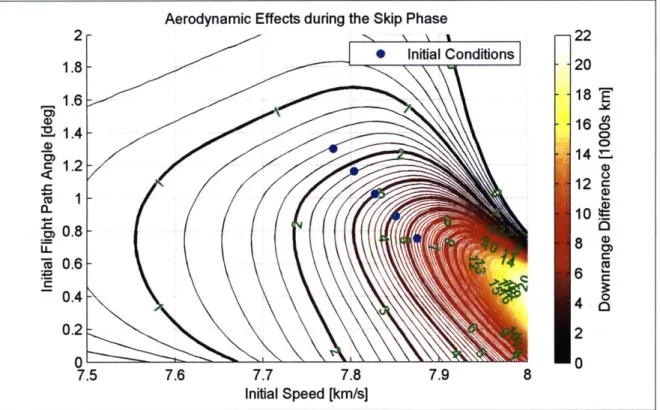
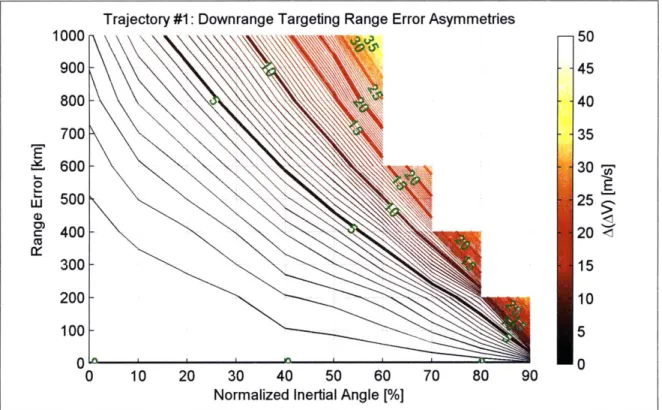
3-5 Asymmetrical minimum impulsive AV with respect to range error . . 63

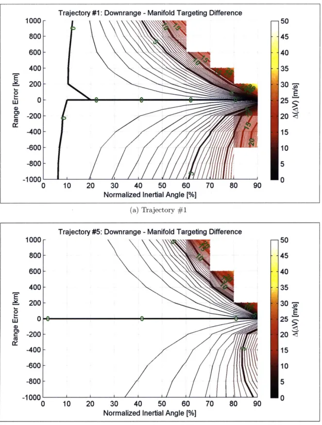
3-6 Difference between class 1 and class 5 trajectories . . . . 64

3-7 Range correction capability for high and low energy trajectories . . . 66

3-8 Manifold targeting to achieve a landing target . . . . 69

3-9 Minimum impulsive AV to target a manifold . . . . 70

3-9 Minimum impulsive AV to target a manifold (cont'd) . . . . 71

3-9 Minimum impulsive AV to target a manifold (cont'd) . . . . 72 3-10 Differences between targeting a downrange location versus a manifold 74

PEG solution AV to target a manifold . . . . PEG solution AV to target a manifold (cont'd) . . . . PEG solution AV to target a manifold (cont'd) . . . . Example of corrected trajectories using PEG to target a manifold PEG solution AV with a constrained altitude . . . .

PEG solution AV with a constrained altitude (cont'd) PEG solution AV with a constrained altitude (cont'd)

Example of corrected trajectories using PEG and a cons Summary of the Monte Carlo results . . . .

Nominal skip trajectories . . . . Histogram of AV required . . . . Histogram of AV required (cont'd) . . . . . .. Histogram of AV required (cont'd) . . . . Scatter of AV required for trajectory #3 . . . . Scatter of AV required for trajectory #3 (cont'd) . . . Scatter of AV required for trajectory #3 (cont'd) . . . Scatter of residual manifold error for trajectory #3 . . Success rate with increasing thruster force for trajectory

. . . . 93 . . . . 94 . . . . 95 trained altitude 95 . . . . 100 . . . . 101 . . . . 102 . . . . 103 . . . . 104 . . . . 105 . . . . 106 . . . . 107 . . . . 110 #2 . . . . . 112 A-1 Direction of minimum impulsive AV to target a downrange location . A-1 Direction of minimum impulsive AV to target a downrange location

(cont'd) ... . . . . . . . .. A-1 Direction of minimum impulsive AV to target a downrange location

(cont'd ) . . . . . . .. A-2 Direction of minimum impulsive AV to target a manifold . . . . A-2 Direction of minimum impulsive AV to target a manifold (cont'd) A-2 Direction of minimum impulsive AV to target a manifold (cont'd) B-i

B-i B-1

Scatter of AV required for a dispersed atmospheric density . . . . . Scatter of AV required for a dispersed atmospheric density (cont'd) Scatter of AV required for a dispersed atmospheric density (cont'd) 5-1 5-1 5-1 5-2 5-3 5-3 5-3 5-4 5-5 5-6 5-7 5-7 5-7 5-8 5-8 5-8 5-9 5-10 119 120 121 122 123 124 126 127 128 . . .

B-2 B-2 B-2 B-3 B-3 B-3 B-4 B-4 B-4 B-5 B-5 B-5 B-6 B-6 B-6 B-7 B-7 B-7 B-8 B-8 B-8 B-9 B-9 B-9 B-10 B-10 B-10 B-11 B-11 B-11 Scatter Scatter Scatter Scatter Scatter Scatter Scatter Scatter Scatter Scatter Scatter Scatter Scatter Scatter Scatter Scatter Scatter Scatter Scatter Scatter Scatter Scatter Scatter Scatter Scatter Scatter Scatter Scatter Scatter Scatter

residual error for a dispersed atmospheric density for for for for for for for for for for for for for for dispersed dispersed dispersed dispersed dispersed dispersed dispersed dispersed dispersed dispersed dispersed dispersed dispersed dispersed.

atmospheric density (con atmospheric density (con spacecraft mass . . . . . spacecraft mass (cont'd) spacecraft mass (cont'd) lift coefficient . . . . lift coefficient (cont'd) lift coefficient (cont'd) drag coefficient . . . . . drag coefficient (contd) drag coefficient (cont'd) thruster force . . . . thruster force (cont'd) thruster force (cont'd) AV AV AV AV AV AV AV AV AV AV AV AV AV AV AV t'd) 145 'd) 146 . . . 147 . . . 148 . . . 149 . . . 150 . . . 151 . . . 152 . . . 153 . . . 154 . . . 155 . . . 156 . . . 157 . . . 158 required required required required required required required required required required required required required required required for for for for for for for for for for for for for for for a dispersed a dispersed a dispersed a dispersed a dispersed a dispersed a dispersed a dispersed a dispersed a dispersed a dispersed a dispersed a dispersed a dispersed a dispersed spacecraft mass . . . . . spacecraft mass (cont'd) spacecraft mass (cont'd) lift coefficient . . . . lift coefficient (cont'd) lift coefficient (cont'd) drag coefficient . . . . . drag coefficient (cont'd) drag coefficient (cont'd) thruster force . . . . thruster force (cont'd) thruster force (cont'd) initial velocity . . . . . initial velocity (cont'd) initial velocity(cont'd) . . . . 129 . . . . 130 . . . . 131 . . . . 132 . . . . 133 . . . . 134 . . . . 135 . . . . 136 . . . . 137 . . . . 138 . . . . 139 . . . . 140 . . . . 141 . . . . 142 . . . . 143 . . . . 144 residual residual residual residual residual residual residual residual residual residual residual residual residual residual error error error error error error error error error error error error error error .

B-12 Scatter of residual error for a dispersed initial velocity . . . . 159

B-12 Scatter of residual error for a dispersed initial velocity (cont'd) . . . . 160

List of Tables

2.1 CEV aerodynamic properties during hypersonic flight . . . . 40

2.2 Summary of simulation parameters . . . . 47

3.1 Skip trajectory initial conditions . . . . 50

3.2 Minimum AV search dimensionality... . . . . . . . 55

3.3 Percent differences between minimum AV search methods . . . . 58

3.4 Initial semimajor axis of each trajectory . . . . 64

3.5 Range correction capability with 40 m/s of AV . . . . 67

3.6 Manifold parameters.. . . . . . . . 68

5.1 M onte Carlo dispersions . . . . 98

List of Symbols

Subscripts

()

Earth-centered, inertial frame

()F Earth-centered, Earth-fixed

frame

)L

Local vertical/local horizontal. frame

()s Stability frame

Oref Reference variable

()g

Gravity quantity

()a

Aerodynamic quantity

()t

Thrust quantity ()T ()D ()L

(o

Of

Ogo

()d

()r

() h Oe Superscripts ()- Inverse Total quantity Drag quantity Lift quantity Initial quantity Final quantity Quantity-to-go Desired quantity Radial quantity Horizontal quantity Error quantity ()T Transpose Accents

First time derivative Second time derivative

Unit vector

Normalized variable

First coordinate vector Second coordinate vector

Third coordinate vector Coordinate Triads

Physical Parameters t r V a z h p m S F AV Isp a Iy 63

At

yG) re ) we CL CD L/D BN T A Time Radial distance Speed Acceleration Downrange distance Altitude Atmospheric density Mass Surface area Thruster force Change in velocity Specific impulse Angle of attack

Flight path angle Bank angle

Thrust direction angle Thrust direction vector

Gravitational parameter of Earth

Radius of Earth

Rotational frequency of Earth Lift coefficient

Drag coefficient Lift-to-drag ratio Ballistic number

Transformation from frame A to frame Z

Longitude

Second gravitational harmonic Semimajor axis Mean Standard deviation Thrust integral Thrust integral Thrust integral Thrust integral

Partial derivative of A with respect to Z

Chapter 1

Introduction

Exploration has long been a part of the human endeavor. The latest incarnation of this quest has been the manned exploration of our solar system. What began in the early 1960s under the inauspicious haze of the Cold War with the Soviet Vostok and Voskhod missions and the American Mercury and Gemini missions has, in the past decade, turned toward more multinational cooperation as demonstrated with the International Space Station. This massive space structure has brought together the once competing Soviet/Russian and American space agencies along with those of Canada, Japan, Brazil and the eleven member nations of the European Space Agency. However, with completion of the ISS on the horizon and retirement of the Space Shuttle eminent, NASA has once again been steered towards the target of putting humans back on the Moon. The plan is to return to the Moon but with the intention of setting up a permanent presence and developing needed experience to further the footprint of human civilization to other planets in the Solar System, namely Mars.

It may seem that returning to the Moon would be pointless and relatively easy considering that this was done nearly forty years ago. That assumption proves to be incorrect as the forty year hiatus has caused a loss of capability in designing human-based exploration missions throughout the industry. In addition, there are much broader mission goals for the modern system that weren't present or considered during the design of the Apollo spacecrafts. Among these is the requirement for the

entry vehicle to be capable of performing extended range landings during a return to Earth from the Moon. This requirement is necessitated by an increased attention to safety and the desire to allow the astronauts to return safely to the surface of Earth at any time during a mission without the need to wait for precise alignment between the Moon launch site and the Earth landing site. However, a capsule shape complicates this process because it has a low lift-to-drag ratio which reduces the range capability of the spacecraft for direct entries. Therefore, some sort of maneuver must be performed during entry to extend its capability to the desired ranges. This is what has brought about the concept of performing skipping entries as a method to achieve the required capability. These maneuvers form the basis of this thesis and the work herein.

1.1

Presidential Vision

On January 14, 2004 President George W. Bush laid the groundwork for the future of NASA and American space exploration in what he called his "New Vision for the Space Exploration Program"

[1].

In his speech he made public a plan to put America back on the Moon by 2020. This includes the completion of the International Space Station to fulfill our responsibility to that project and the fifteen international partners. It also entails retiring the Space Shuttle after 30 years of service to make room for the next generation of launch vehicles. The next spacecraft, named the Crew Exploration Vehicle (CEV), will be tested beginning in 2008, during the final days of the Space Shuttle. This vehicle will assume the role of ferrying astronauts to the International Space Station but will also be capable of transporting them beyond Earth orbit. He proposed how the experience gained by living and working on the Moon for extended periods of time will enable humans to extend their reach to Mars as well. The establishment of a lunar base could produce significant reductions in the cost of future space exploration. It might be possible to process the lunar soil for useful applications like rocket fuel or breathable air. He emphasized that this progress will be steady and made one step at a time.

The speech draws upon historical references to pre-industrial exploration by ad-venturers such as Meriweather Lewis and William Clark. He goes on to explain that America's adventure into space is a modern version of Lewis and Clark expedition. He continues to state that exploration is a part of the American character and that it has brought tangible improvements to the American life. Even with all the suc-cesses of NASA with the Space Shuttle, robotic exploration of the solar system, and numerous telescopes such as the Hubble Space Telescope; no human has been further than 386 miles upward since 1974. This is roughly equivalent to the distance between Boston and Washington, D.C. or between San Francisco and Los Angeles. The future of space exploration will use these robotic trailblazers to send images and scientific data that will lay the foundation for the arrival of humankind.

Since this announcement there has been a lot of engineering put into designing a system that can take humans to the Moon and beyond while maintaining a level of safety that is demanded in the wake of the Columbia tragedy. The current pre-liminary design of the CEV is documented in detail in "NASA's Exploration System Architecture Study"

[2].

A key aspect of this design is a move away from the Shuttle-like lifting bodies with delta wing planforms to an Apollo derived capsule shape with a large heat shield belly. This design was chosen for a variety of reasons not the least of which are safety and efficiency. The conic shape allows the capsule to be placed atop a launch vehicle which improves the safety of the crew and allows for a method of escape in the event of an accident during launch. It is also a more efficient use of structural material because the wings of the Shuttle are essentially dead weight beyond the atmosphere and therefore ill-suited for interplanetary travel. Another key design element is the separation of cargo lifting operations and crew transportation. This adds another factor of safety because the crew launch vehicle can be designed specifically its intended purpose. This will also reduce cost of launching cargo because the launch vehicle does not need to carry as stringent of a safety rating as the crewed launch vehicle.

Perhaps the aspect of the design most relevant to this thesis is that the CEV is designed to perform an atmospheric skip entry. An atmospheric skip entry trajectory

is defined, for the purpose of this thesis, to be a trajectory that upon entering the atmosphere has enough energy that the trajectory effectively lofts the spacecraft upwards momentarily before returning to back to Earth. A skip is traditionally defined to begin and end the entry interface which for Earth is approximately 120 km altitude. The atmospheric skip entry trajectory concept is illustrated in Figure 1-1. A common analog that is frequently stated is that of skipping a stone off the surface of a pond. If the skip is properly controlled, it can be used to increase the range capability of the entering spacecraft. This proves to be very advantageous for low lift-to-drag ratio vehicles such as the CEV concept. The trajectories created by skip entry maneuvers form the basis of this thesis.

1.2

Background

The concept of atmospheric skip entry trajectories is not entirely new. The idea has been around since the beginning of manned space exploration. The Apollo pro-gram used a guidance algorithm that was designed to perform such a maneuver [3]. However, the documentation doesn't show any evidence that this capability was ever tested beyond the feasibility stage and subsequent testing has shown that the perfor-mance of the entry guidance algorithm is less than satisfactory when attempting to perform this maneuver. The Soviets performed the first successful skip entry with the Zond 6 circumlunar spacecraft [4] [5] [6]. It was decided to perform such a maneuver for two reasons. The first was to reduce the excessive g-loads placed on the crew dur-ing a ballistic entry from the moon. The other, and perhaps more politically drivdur-ing, factor was that it wasn't possible to land in Soviet territory from a lunar ballistic return. The Zond 6 return was completed with spacecraft reaching an altitude of 45

km during its first entry while decelerating from 11 km/s to 7.6 km/s and experiencing

g-loads of only 4 to 7 g's. Unfortunately, a pressure sensor onboard the spacecraft failed and it crashed after the parachutes deployed too early

[7].

It is interesting to note that until the U.S.S.R. opened up under Glasnost, the fact that the Zond 6 mis-sion ended in disaster was not known because a few photographs that were recovered

Skip Phase

From

(a) Polar view of a skip trajectory

Downrange

(b) Skip trajectory phase definitions

Figure 1-1: An example of an atmospheric skip entry trajectory

from the wreckage were shown to the public and was assumed to be proof of success. The next attempt at a circumlunar mission was made a few weeks after Apollo 8 in January of 1969. There was some debate within the Soviet space command over whether or not to place a crew on this mission. It was decided against placing a crew onboard since a simple fly-by of the Moon would not look good compared to the ten orbits achieved by Apollo 8. This decision proved to be fortuitous for the possible cosmonauts as the launch failed when the second stage exploded and thus the mission remained unnamed. The next Zond mission, Zond 7, was the only Russian mission which could have carried humans successfully around the Moon and landed safely back on Earth. Despite public claims by the Soviet cosmonauts that a manned lunar landing would take place by early 1970, it was decided to continue testing the Zond spacecraft unmanned. Zond 7, launched on August 8, 1969, a couple weeks after the Americans' historic landing on Moon with Apollo 11. It followed the trajectory of Zond 6 and likewise performed a skip entry but landed successfully in what is now Kazakhstan south of the town of Kostanai (then spelled Kustanai) six days after it launched

[4] [5] [7).

There have been a few subsequent papers that focus on guidance algorithms for such a maneuver.

Reference [8] discusses a rudimentary guidance algorithm for the "skipout" phase of a skip trajectory. The "skipout" phase was defined at the latter half of the first entry as defined in Figure 1-1b. The optimal guidance solution is found using a conjugate gradient method to converge to a reference trajectory. The simulation used was straightforward and relatively simple; it is essentially a point design and does not include any sensitivity analysis. The skip phase target range of the trajectory considered is 16,924 nmi (approximately 31,000 km) or more than three quarters around the globe. This is substantially larger than the skip considered by other references or this thesis.

Reference [9] proposes using skip trajectories for aeroassisted orbital transfer. The guidance algorithm proposed uses an analytic predictor-corrector which solves for the final state of the vehicle using a closed form expression. This expression is an approx-imation of the flight dynamics derived from using the method of matched asymptotic

expansions. It shows good performance for a Martian aerocapture trajectory. How-ever, this technique does not appear to be well suited for the aeroassisted transfer trajectories discussed in the paper as it seems as though this maneuver would require more fuel to enter and exit the transfer orbit than an equivalent Hohmann transfer. This solution would clearly require less time than a Hohmann transfer but time is generally unconstrained for these types of missions and fuel mass is a system driver.

Perhaps the most recent addition to the literature and certainly the most pertinent to this thesis is Reference [10]. The work presented covers an aerodynamic guidance algorithm developed for a low lift-to-drag ratio spacecraft such as the CEV. A key feature of this work is the ability to perform a skip maneuver to allow a low L/D vehicle to achieve the extended range landings. This is done by augmenting the Apollo guidance algorithm with a numeric predictor-corrector to increase the landing accuracy. A numeric predictor-corrector solves for the final state of the spacecraft by integrating the equations of motion forward in time. This method is generally more accurate than an analytic predictor-corrector but can take substantially more computational effort.

Reference [10] covers quite a bit of the entry problem and is an excellent reference on the inner workings of the original Apollo guidance algorithm. While it presents an algorithm for reaching a wide variety of targets, it also offers a look in the physics of a skip entry. Besides extending the landing range capability, another advantage with skip entries is that the maximum g-load can be reduced. This benefit arises because the spacecraft is able to extend the deceleration over a longer period of time. This effect creates a gentler entry environment for the astronauts onboard that may be injured or simply weak from spending an extended period of time in a reduced gravity environment. One problem with skip trajectories is that they tend to increase the total heat load due to their extended flight time through the atmosphere. However, the maximum heat rate is achieved during the first entry and, therefore, is independent of the desired range.

1.3

Motivation

The resulting algorithm designed in Reference [10] performs very well for the set of landing ranges that was examined. One caveat to this is the simulation was performed using only translational dynamics. The problem is that this neglects the effects of the rotational dynamics which enhance the fidelity of the model. The performance of the algorithm actually degrades because the inclusion of rotational dynamics complicates the guidance problem and results in poorer precision performance.

Some preliminary follow-up to Reference [10] using a six degree-of-freedom sim-ulation has shown that in fact large errors can occur when targeting the farthest of the landing ranges. These errors can be caused by problems within the algorithm design itself but it is more likely that they are the result of imperfect control and the uncertainties in the newly included rotation axes. Regardless of the cause of the errors, a method for correcting them without the use of aerodynamic control is needed. This need can be met by the addition of a propulsive guidance algorithm performing a AV maneuver during the skip portion of the entry. This complements the aerodynamic guidance perfectly because they operate in separate regimes. The bank-to-steer guidance proposed in Reference [10] works extremely well when the at-mosphere is thick and the entering spacecraft can exchange energy and momentum with the atmosphere. This unfortunately creates a problem when the atmosphere is thin as it is during the skip portion of a long range trajectory. A propulsive algorithm compliments this because it works best when the atmosphere is thin since it is neces-sary to reorient the vehicle to point the thrusters in the right direction for a propulsive maneuver. Figure 1-2 qualitatively shows this distinction between aerodynamic and propulsive guidance.

The algorithm from Reference [10] also demonstrates the capability to choose a "high loft" or "low loft" trajectory. The main difference between these types of trajectories is that the "high loft" trajectories reach a higher maximum altitude during the skip phase of the entry than those of the "low loft" variety. However, there are other differences between the trajectories which point to differences in their individual

Entry Interface

Figure 1-2: Effective regimes for aerodynamic and propulsive guidance

energy levels and flight path angles. The reasons for choosing one type of trajectory over the other are discussed but the primary reason is to reduce the range sensitivity of the skip phase due to aerodynamic effects that exist in the "low loft" trajectories as will be discussed later. This, in actuality, exacerbates the problem of using only bank-to-steer guidance during the skip phase because a "high loft" trajectory spends more time in the uppermost regions of the atmosphere. This accentuates the need for a propulsive guidance algorithm during the skip phase because without it the spacecraft is essentially flying open-loop and can very easily drift off course. One advantage to using the high loft trajectories is that they allow for more time perform the propulsive maneuver. The reason for this is because the spacecraft

Will

likely need to reorient and point the thrusters in some other direction to achieve the desired change in velocity. However, for a reasonable thruster size, it will not be possible to reorient whenever it might be necessary. This means that the aerodynamic moments must drop below some specified level, depending on the size of the thrusters, before it ... ... .... ...

is possible to reorient the spacecraft. This only occurs when either the atmospheric density or velocity becomes small enough. The velocity is near orbital speed so the prerequisite that remains is the density which becomes small when the spacecraft is high in the atmosphere.

The aforementioned problem and its intricacies lay the foundation for the work encompassed by this thesis. That being the design of a propulsive guidance algorithm to correct for errors during the skip portion of the trajectory that would otherwise create large landing inaccuracies.

1.4

Objective

The objective of this thesis is to implement and evaluate a propulsive guidance al-gorithm for use during the skip phase of a lunar return trajectory. The skip phase becomes increasingly prominent as the landing range is increased, therefore the longest landing ranges are considered. The vehicle will be based upon the CEV design concept which is a low lift-to-drag ratio capsule similar in shape to the Apollo capsule.

The guidance algorithm will be based upon the Powered Explicit Guidance (PEG) law that was developed for the Space Shuttle in the 1970s. It was originally devel-oped for ascent and later revised to perform exoatmospheric maneuvers such as plane changes and orbit raising and lowering as well as deorbit targeting for the descent phase. It has the advantage that it has been verified and validated through its many uses in the Space Shuttle program. Although none of the current implementations are completely appropriate for the problems encountered by a spacecraft in a skip trajectory, all contain certain elements that are crucial to this new derivative. The operating regime of this problem is most clearly related to that of the orbital maneu-vering version. However, this version does not contain the ability to target a specified downrange location and it does not account for any atmospheric effects. The ascent version of PEG does account for the atmospheric effects but it, too, has no ability to specify the downrange termination condition and its operational regime is not appro-priate. The deorbit targeting version does allow for the targeting of a landing site but

its operating regime is inappropriate as well. Clearly each version of the algorithm works very well for its intended purpose. However, it is not a trivial task to include the atmospheric effects from the ascent version with the targeting capability of the deorbit version into the operating regime of the orbital maneuvering version.

The first step is to define a set of nominal reference trajectories representative of a reasonable range of atmospheric exit conditions produced by the initial aerodynamic guidance. This set is separated into several different "classes" of trajectories. The term "classes" is used because the skip phase of the entry can be shaped depending on a number of parameters. This idea is very similar to the "high" and "low" loft tra-jectories mentioned earlier but it will be necessary to explore what happens between these two extremes. It is clear that there are many possible trajectories to reach a

desired landing target. These trajectories can be classified in terms of their individual energy levels during the skip phase. The higher energy trajectories are ones that enter the skip phase with a greater velocity and a shallower flight path angle. Conversely, the low energy trajectories enter the skip phase with a lower velocity and a high flight path angle. The high energy trajectories are more desirable from a pure capability standpoint because they allow for more variation in the final phase entry condition and thus a broader range of correction. However, the low energy trajectories are more desirable from a feasibility standpoint since it allows for more time to perform the corrective maneuver because they travel higher out of the atmosphere. Both high and low energy trajectories offer advantages over the other and these will be examined

along with a number of the "shades of gray" in between.

A preliminary analysis is completed using an impulsive AV. This gives a good lower bound on the amount of AV (and hence fuel) needed to correct for a given amount of error. The problem with getting realistic approximations from impulsive analysis solutions is that they require extremely high thrust levels to achieve the specified AV in a very short amount of time. Therefore, using more reasonably sized thrusters makes the time (and hence the AV) required to perform the necessary cor-rections increase when compared to the impulsive case. The result of this analysis will include a way of determining the thruster size and/or number needed depending

on vehicular and environmental constraints.

Once the guidance algorithm has been developed and tested against a represen-tative set of skip trajectories it is necessary to quantify the performance under a variety of conditions. This will require defining a set of vehicle and environmental uncertainties. A Monte Carlo analysis will then be performed to test the sensitivity of the algorithm to unanticipated variations in the vehicle and environment. This defines the robustness of the design and is a measure of the quality of the design.

1.5

Overview

This chapter gives a broad overview of using skip trajectories during entry and pro-vides an introduction to the topic of the thesis. Chapter 2 propro-vides an explanation of the physics of the problem and the design of the spacecraft used during this thesis. Chapter 3 covers the results of a preliminary analysis using an impulsive AV to find a lower bound to the problem. Chapter 4 discusses the design of the guidance algorithm and an overview of the Powered Explicit Guidance algorithm that forms the basis of the algorithm presented here. Chapter 5 presents the results of a Monte Carlo analy-sis using the newly designed guidance algorithm. Finally, Chapter 6 summarizes the work presented in this thesis and gives some suggestions for future avenues of study.

Chapter 2

Simulation Environment

In order to begin the analysis, a number of parameters must be defined. This will bound the scope of the thesis to validity only in the neighborhood of where the assumptions hold. To that end, it is important that the assumptions be as broad and unrestrictive as possible so the solutions are not a point design. However, making the assumptions too broad will make the problem too complicated to be solved with one thesis. Therefore, assumptions are tuned for a scope that produces a result that is significant and useful.

Many tools can be used when designing a simulation. The tool of choice for this problem is MATLAB version 7.2 produced by The MathWorks, Inc. MATLAB contains a complete development environment with many included functions and the

ability to extend its capability to specific areas of interest through the use of toolboxes and user-defined libraries of functions. One such toolbox is Simulink. It allows the designer to develop dynamic models of systems using an intuitive graphical interface to represent the various components of the system and their connections. Once a system has been developed, the designer can simulate the dynamics of the system with the press of a button. A designer can then see how the system behaves and how that behavior compares to the nominal design. This capability of being able to rapidly design and test an idea is invaluable in engineering and science.

2.1

Coordinate Frames

There exist multiple ways to formulate any given problem depending on the coordinate frame desired. However, the choice of the coordinate frame can greatly reduce the complexity of a problem and allow for deep insights into the dynamics of the system. For the purpose of this thesis, four different coordinate frames are used: an inertial frame, an Earth-fixed frame, a local vertical/local horizontal frame, and a stability frame. To disambiguate a vector in each frame the subscripts 0), OF, OL, and

()s

are used; respectively. Due to their similarities, the coordinate frames are presented in two groups based upon where the origin is located. The first group is the Earth-centered frames which include the inertial and Earth-fixed frames. The other group is the spacecraft-centered frames which include the local vertical/local horizontal frame and the stability frame.

2.1.1

Earth-centered

The Earth-centered inertial frame is used primarily for the integration of the equations of motion presented later in Section 2.4. It is represented by the unit vectors ir, ji, and k₁. The ij axis points to the intersection of the equator and the prime meridian (zero latitude and longitude) at t = 0. The k, axis points toward the North Pole

(900 North latitude) and jr completes the frame in a right-handed sense (zero latitude and 90' East longitude). A vector u can then be expressed as

u = xi₁ + yjj + zk₁. (2.1)

This vector u can be any quantity that has magnitude and direction such as position or velocity.

The Earth-centered Earth-fixed frame is used to measure the spacecraft's position and velocity relative to a fixed point on the Earth. This is needed when discussing the range to a landing site and calculating the speed of the spacecraft relative to the atmosphere used in aerodynamic calculations. It is related to the Earth-centered

____ "4 W~JF

S t

F

Figure 2-1: Earth-centered coordinate frames

inertial frame by a rotation about the polar axis, kF, with a period identical to that of the Earth. The

IF

and $F axes stay fixed to the Earth as it rotates. This is distinguished from the Earth-fixed inertial frame by the following relations

i1(t = 0) = 1F

(2.2)

j1(t = 0) =JF

(2.3)

I=kF. (2.4)

It should be clear that the Earth-fixed and inertial frames are identical at the be-ginning of the simulation, after that they oscillate with a period identical to Earth's rotational period. The inertial and Earth-fixed frames are shown in Figure 2-1 at some time, t, where we is the Earth's rotational frequency.

2.1.2

Spacecraft-centered

The local vertical/local horizontal is centered on the spacecraft and used to define the direction of motion of the spacecraft. This is defined as the flight path angle and is the angle above the local horizontal and in the direction of the velocity vector. The

local vertical is defined to be in the direction of the position vector so

JL (2.5)

where ir is the unit position vector. The local horizontal is defined to be in the downrange direction. Before this position can be defined it is necessary to define the crossrange direction as

kL = -Ih = 1r (2.6)

lV X 1r

where i, is the unit velocity vector and ih is the unit angular momentum vector. Therefore, the local horizontal is defined to complete the right-handed coordinate frame as

IL jL x L = Ih X ir- (2.7)

Then the flight path angle, -y, is defined as

= cos 1 - IL) sign ir ' io (2.8)

where sign is a real-valued function which is defined such that

z =

I

zI signz. (2.9)

Therefore, the flight path angle is defined such that

signh sign y, V7- E (-7, 7) (2.10)

where h is the altitude rate.

The stability frame is also centered on the spacecraft and is used to define the directions in which the aerodynamic and propulsive forces are acting. The unit vector triad can be defined arbitrarily with respect to the body as long as they are kept fixed thereafter. For the purpose of this thesis it is beneficial to define this with respect to the velocity and the aerodynamic forces created by the velocity. Therefore, the is axis

r

JL

ee

ks

Figure 2-2: Spacecraft-centered coordinate frames

is defined into the wind (assuming no sideslip) so it is aligned with the Earth relative velocity and in the negative direction of the drag vector. The ks axis is defined in the negative direction of the lift vector (assuming straight and level flight) in the r-v plane. The

js

axis completes the frame in a right-handed sense. This definition gives a positive angle of attack when the vehicle is pitched up.

The local vertical/local horizontal and stability frames are shown with respect to each other and the position and velocity vectors in Figure 2-2.

2.1.3

Coordinate Transformations

The definitions of the coordinate frames establish a convenient basis for analyzing the dynamics of the spacecraft under a variety of different conditions. A problem with using separate frames is that it isn't immediately clear what the spacecraft is doing in another frame. In addition, the equations of motion must be specified in a frame that

is non-accelerating and non-rotating in order for Newton's Second Law to be valid. The inertial frame is by definition one such frame. Therefore, it is necessary to define a method for transforming vectors from their natural frame to an inertial frame. To perform this operation, a transformation matrix, T, from frame A to frame Z such that

rz = rA. (2.11)

A transformation matrix has the benefit of being an orthonormal basis. This means that the reverse transformation can be computed by taking the transpose of T instead of requiring its inverse. Therefore, the reverse transformation from frame Z to frame

A is

1 (TZ) T TA

rA = (=T) rz rz = Trz. (2.12)

It is also possible to perform a series of transformations consecutively. Therefore, it is possible to transform r from frame A to frame Z through frame M with

rz = TATIrA. (2.13)

One should note that serial transformations are non-commutative so that

T7T'

#

TAITi. (2.14)

With the rules of coordinate transformations defined, it is now possible to establish the transformations needed for this thesis. The transformation from Earth-fixed to

inertial is a simple rotation about their k axes so that TFis

cos0 sinO 0

1

-sin 0 cosO 0 (2.15)

0 0 1

where 0 = Wet for some time t and is the commonly known as the longitude.

frame, T/, is established by some key unit vectors as L) (2.16) -where

iL)

(L, X (L) (2-17) (2.18) kL -(h

(v

X 1r (2.19) lv X 1r

The transformation from the stability frame to the local vertical/local horizontal frame is a series of rotations starting with a rotation about -kL through y, the flight path angle followed by a 90 degree rotation about IL such that

1 0 0 Cos -sin - 0 cosy -sin 0

s 0 0 1 siny cosy 01

0

0 1

.

(2.20)

0 -1 0 0 0 1 -sin - Cosy 0

With these three transformations defined and the transformation properties rep-resented by Equations (2.12) and (2.13), all possible transformations can be found between the four coordinate frames discussed in this chapter.

2.2

Environment Model

The environment includes all things that are generally thought to be a part of Nature. This means that anything outside of the vehicle that can interact with it should be included within the simulation to maximize its fidelity. This might include things such as the atmosphere of Earth, the Earth's gravity field, the Earth's magnetosphere, or even the solar wind. The dominating components of the environment for this problem are the atmosphere and gravity. The magnetosphere only affects objects with

high electromagnetic properties such as charge or current and even still this is only significant while in orbit. The solar wind tends to dominate when things have a high surface area and are in interplanetary space. For these reasons the magnetosphere and solar wind are assumed to be negligible and are thus ignored.

2.2.1

Atmosphere Model

The atmosphere used for this thesis is based upon the 1962 U.S. Standard Atmo-sphere [11]. It gives a prediction of the expected value for physical atmospheric properties such as temperature, pressure, and density. The model extends up to

700 km which is easily encloses the operational regime of the problem presented in

this thesis.

The wind is assumed to be negligible at the altitudes of interest, because even though the winds may be high, the density is small enough to safely ignore the effects of wind on the spacecrafts trajectory. The atmosphere is assumed to be fixed relative to the surface of the Earth therefore it remains coincident with the Earth-centered Earth-fixed frame.

The atmosphere is also assumed to be entirely in the continuum flow regime. While the trajectories do spend a substantial portion of time in the transitional regime between those of continuum and free molecular flow, the effects have shown to be minimal over the relatively short period of time of the skip phase. Therefore, the rarefied atmospheric effects and the required adjustments to the aerodynamic coefficients are assumed to be negligible.

2.2.2

Gravity Model

The gravity model used in this thesis is a simple Newtonian gravity field with its familiar inverse-squared relation. The acceleration due to gravity in a Newtonian gravity field is

where ye is a constant known as the gravitational parameter of Earth (398,600 km23/₈2)

r is the distance between the spacecraft and the center of Earth, and i, is the unit

vector pointing in the direction of the spacecraft.

A more complicated model for the gravity is unnecessary for the level of fidelity needed for this thesis because the next higher order model includes J₂, the second

gravitational harmonic. Its magnitude is on the order of 10- and only has a signifi-cant effect on spacecraft that orbit for long periods of time. Given that the problem presented in this thesis is less than one orbit it is safe to assume that the effects of

J2 are negligible.

2.3

Vehicle Model

The vehicle chosen for the basis of this thesis is the current Crew Exploration Vehi-cle (CEV) design concept documented in Chapter 5 of Reference

[2].

This chapter includes all the relevant information necessary to define a simplified model of the vehi-cle. It also includes the details of some interesting trade studies that were completed to define the shape and capabilities of the CEV. The shape that was shown to be the best overall design was a design that is essentially an enlarged Apollo Command Module. The shape is shown in Figure 2-3. It shows a 5.5 m diameter blunt body with a 32.50 sidewall. The original Apollo Command Module had 3.9 m diameter and a 32' sidewall. The purpose for enlarging the shape is to increase the pressurized volume by nearly a factor of three. This allows for larger crews but also more volume

per crew member which is necessary for long duration missions.

The mass of the CEV on a return from the Moon is assumed to be 9600 kg which includes a 100 kg margin allotted to sample returns from the lunar surface. The cross-sectional area of the of the CEV is easily calculated from the diameter stated above, to be 23.76 m2 (S = 1ird2). For comparison, the Apollo Command Module weighed

in between 5500 kg and 5900 kg, depending on the mission, and had a cross-sectional area of 11.95 M2

.

3.617

1.00

6.476 0.275

2.75

Figure 2-3: CEV shape [2]

Table 2.1: CEV aerodynamic properties during hypersonic flight [10]

M atri, (deg) CD CL L/D BN (kg/m2) 4 27.20 1.1444 0.50069 0.43751 353.08 6 26.68 1.1651 0.47066 0.40397 346.81 10 25.94 1.1886 0.46326 0.38975 339.95 18 24.18 1.2307 0.44825 0.36422 328.32 25 23.68 1.2446 0.43760 0.35160 324.66 32.2 23.22 1.2507 0.43513 0.34791 323.07

regime (Al > 5) and initial tests have shown the Mach number to be at the upper end of that regime (Al > 15). This is expected given that a skip occurs when the velocity is near orbital speeds. It should also be noted that it is assumed that the spacecraft maintains flight at a trim angle angle of attack (atrim) when not performing a propulsive maneuver. A vehicle's lift-to-drag ratio is driven by a number of factors. One such factor is the location of the center of gravity. The center of gravity for the CEV model used in this thesis is chosen in accordance with Reference [10] where it was selected to establish a trim lift-to-drag ratio of 0.35 during the hypersonic regime. The aerodynamic properties of the CEV in the hypersonic regime are shown in Table 2.1 where M is the Mach number, atrim is the trim angle of attack, CD is

the drag coefficient, CL is the lift coefficient, L/D is the lift-to-drag ratio, and BN

is the ballistic number. These values are slightly different from those of the Apollo Command Module but this is due to a difference in the location of the center of gravity.

The CEV will also have the ability to perform a propulsive maneuver during the skip phase. The propulsion system design is also discussed in Reference

[2].

It states that the assumed AV for entry maneuvering is 10 m/s and for the skip phase correction burn is 40 m/s. The thrusters are chosen to be two 100 lbf (445 N) liquid fuel rockets with an IP of 274 s. It is assumed that these thrusters are positioned in such a way to provide only a translational force without any resultant moment.

2.4

Equations of Motion

The equations of motion are a set of equations that describe the dynamics of the system. They can vary depending on the accuracy of the model and the complexity of the problem. In the case of the propulsive entry problem the equations are non-linear and differential. The most basic representation of the equations of motion is

aT = a + aa+ at (2.22)

where i is the second time derivative of the position, aT is the total acceleration, a9

is the acceleration due to gravity, aa is the aerodynamic acceleration, and at is the acceleration from the thrusters.

The acceleration due to gravity is already shown in Equation (2.21) but written in terms of the local vertical/local horizontal frame it becomes simply

a9 = jL- (2.23)

r

The aerodynamic acceleration is the vector sum of the drag and lift accelerations

where the magnitude of aD is calculated from

aD = q (2.25)

BN and the magnitude of aL is Simply

L

aL = -aD. (2.26)

D

The variable q in Equation (2.25) is known as the dynamic pressure and is the apparent pressure from moving through a fluid. It is defined as

q = PV2e (2.27)

where p is a function of altitude as defined in Subsection 2.2.1 and vre is the atmo-spheric relative speed.

The acceleration from drag always acts opposite the direction of motion relative to the wind, -is, and the lift acceleration is defined to be in the

js-ks

plane so it is perpendicular to the drag. The bank angle, 0

b, is defined such that when it is

zero the lift vector points in the -ks direction. Therefore, in the stability frame, the combined aerodynamic acceleration becomes

-1

(aa)s =

sinb

]

.

(2.28)

The thrust acceleration is defined as

at

At

(2.29)

m

where Ft is the magnitude of the force applied by all the thrusters firing (in this case 2 x 100 lbf), m is the spacecraft mass, and At is the unit vector in the direction of the thrusters.

For this thesis it is assumed that the thrusters remain in the r-v plane and thus no side force is created. Therefore, it is convenient to define the vector At in terms of the local vertical/local horizontal frame by simply breaking the vector into its components.

cos

1

At = sin1

#

(2.30)

0

where 3 is the thrust direction angle which is the angle between At and the local horizontal. It uses the same sign convention as the flight path angle.

By combining Equations (2.21), (2.28), and (2.31), the total acceleration becomes

0

1

cos1

(ar) TL P -1 sin Ob + t- sin (231)

r2- BN TT

0

-)T

CO

jL

sb

0

- -L - D __-L

and the position and velocity vectors are defined by

V = V +0 aT dt (2.32)

0t/

r = r +0 v dt (2.33)

where ro and vo are the initial position and velocity, respectively, and t1 is the final

time.

2.5

Boundary Conditions

The initial conditions and the final termination condition must be defined before the equations of motion can be integrated. These are represented in Equations (2.32) and (2.33) as ro, vo, and tf.

The initial conditions ro and vo are the position and velocity at the start of the skip phase. The skip phase is defined in accordance with the Apollo guidance