V2477 Cyg: a W-type contact eclipsing binary

(1)

Publisher’s version / Version de l'éditeur:

Information Bulletin on Variable Stars, 2017-01-02

READ THESE TERMS AND CONDITIONS CAREFULLY BEFORE USING THIS WEBSITE. https://nrc-publications.canada.ca/eng/copyright

Vous avez des questions? Nous pouvons vous aider. Pour communiquer directement avec un auteur, consultez la première page de la revue dans laquelle son article a été publié afin de trouver ses coordonnées. Si vous n’arrivez pas à les repérer, communiquez avec nous à [email protected].

Questions? Contact the NRC Publications Archive team at

[email protected]. If you wish to email the authors directly, please see the first page of the publication for their contact information.

Archives des publications du CNRC

This publication could be one of several versions: author’s original, accepted manuscript or the publisher’s version. / La version de cette publication peut être l’une des suivantes : la version prépublication de l’auteur, la version acceptée du manuscrit ou la version de l’éditeur.

For the publisher’s version, please access the DOI link below./ Pour consulter la version de l’éditeur, utilisez le lien DOI ci-dessous.

https://doi.org/10.22444/IBVS.6192

Access and use of this website and the material on it are subject to the Terms and Conditions set forth at

V2477 Cyg: a W-type contact eclipsing binary

Nelson, Robert H.

https://publications-cnrc.canada.ca/fra/droits

L’accès à ce site Web et l’utilisation de son contenu sont assujettis aux conditions présentées dans le site

LISEZ CES CONDITIONS ATTENTIVEMENT AVANT D’UTILISER CE SITE WEB.

NRC Publications Record / Notice d'Archives des publications de CNRC:

https://nrc-publications.canada.ca/eng/view/object/?id=c3368d2f-d3ac-44c2-8df6-5af54dd51590 https://publications-cnrc.canada.ca/fra/voir/objet/?id=c3368d2f-d3ac-44c2-8df6-5af54dd51590

(2)

COMMISSIONS G1 AND G4 OF THE IAU INFORMATION BULLETIN ON VARIABLE STARS

Volume 62 Number 6192 DOI: 10.22444/IBVS.6192

Konkoly Observatory Budapest

2 January 2017 HU ISSN 0374 – 0676

V2477 Cyg — A W–TYPE CONTACT ECLIPSING BINARY

NELSON, ROBERT H.1,2

1_{393 Garvin Street, Prince George, BC, Canada, V2M 3Z1}

email: [email protected]

2_{Guest investigator, Dominion Astrophysical Observatory, Herzberg Institute of Astrophysics, National}

Re-search Council of Canada

The variability of V2477 Cyg (NSV 13016 = NSVS 3227395 = HD 239379 = TYC 3945– 1423–1), amongst many others, was discovered photographically by Hoffmeister (1963) as part of the Sonneberg Survey (Gessner 1966). The former gave coordinates and a finder chart, described the system as a short period variable, and designated it as S 7891. Skiff (1999) identified many Sonneberg variables, amongst them S 7891, giving accurate coor-dinates and associating them with existing names. The first accessible elements (epoch, period) were published by Otero & Wils (2005), who also classified the system as EW, and listed the magnitude range and spectral type. Since then, there have been a number of eclipse timings, but no light curve analysis.

In order to rectify this lack, the author first secured, in April of 2015 and again in September of 2016, a total of 6 medium resolution (R∼10000 on average) spectra of V2477 Cyg at the Dominion Astrophysical Observatory (DAO) in Victoria, British Columbia, Canada using the Cassegrain spectrograph attached to the 1.85 m Plaskett Telescope. He used the 21181 grating with 1800 lines/mm, blazed at 5000 ˚A giving a reciprocal linear dispersion of 10 ˚A/mm in the first order. The wavelength ranged from 5000 to 5260 ˚A, approximately. A log of observations is given in Table 1. The following elements were used for both radial velocity (RV) and photometric phasing:

JD(Hel)MinI= 2457176.2636 + 0.3112515 E (1)

Frame reduction was performed by software ‘RaVeRe’ (Nelson 2009). See Nelson et al. (2014) for further details. The normalized spectra are reproduced in Fig. 1, sorted by phase. Note towards the right the strong neutral iron lines (at 5167.487 and 5171.595 ˚A) and the strong neutral magnesium triplet (at 5167.33, 5172.68, and 5183.61 ˚A).

Radial velocities were determined using the Rucinski broadening functions (Rucin-ski 2004, Nelson 2010b, Nelson et al. 2014). An Excel worksheet with built-in macros (written by him) was used to do the necessary RV conversions to geocentric and back to heliocentric values (Nelson 2010a). The resulting RV determinations are also presented in Table 1. These results were corrected 5.2% up for the 2015 data, but only 1% for the 2016 data (owing to the shorter exposure times) to allow for the small phase smearing. Correc-tion was achieved by dividing the RVs by the factor f = (sinX)/X; where X = 2πt/P , where t denotes exposure time and P denotes the orbital period. For spherical stars, this

(3)

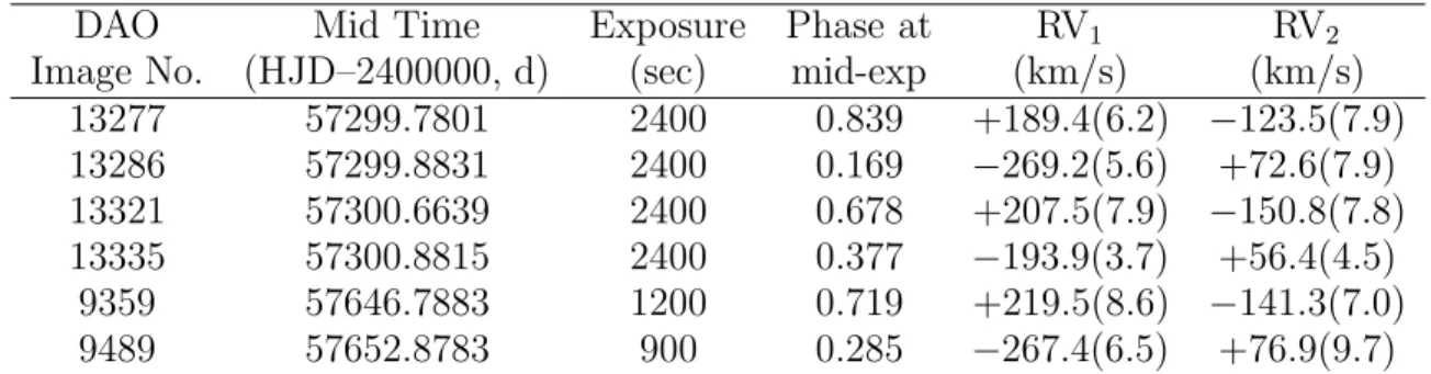
Table 1: Log of DAO observations.

DAO Mid Time Exposure Phase at RV1 RV2

Image No. (HJD–2400000, d) (sec) mid-exp (km/s) (km/s) 13277 57299.7801 2400 0.839 +189.4(6.2) −123.5(7.9) 13286 57299.8831 2400 0.169 −269.2(5.6) +72.6(7.9) 13321 57300.6639 2400 0.678 +207.5(7.9) −150.8(7.8) 13335 57300.8815 2400 0.377 −193.9(3.7) +56.4(4.5) 9359 57646.7883 1200 0.719 +219.5(8.6) −141.3(7.0) 9489 57652.8783 900 0.285 −267.4(6.5) +76.9(9.7)

correction is exact; in other cases, it can be shown to be close enough for any deviation to fall below observational errors. The mean rms errors for RV1 and RV2 are 6.4 and 7.5

km/s, respectively, and the overall rms deviation from the (sinusoidal) curves of best fit is 9.7 km/s. The best fit yielded the values K1 = 256.6(1.1) km/s, K2 = 118.1(1.1) km/s

and Vγ = −30.5(0.6) km/s, and thus a mass ratio qsp= K1/K2 = M2/M1 = 2.17(2).

Figure 1. V2477 Cyg spectra at phases 0.169, 0.285, 0.377, 0.678, 0.719, 0.839 (from top to bottom).

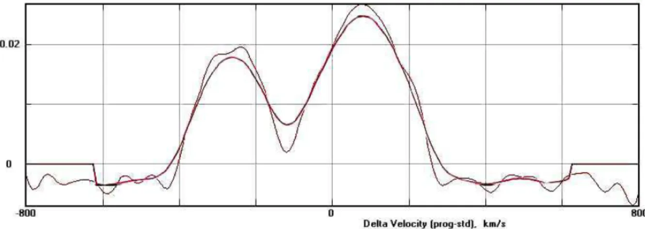
Representative broadening functions, at phases 0.285 and 0.719 are depicted in Figs. 2 and 3, respectively. Smoothing by a Gaussian filter is routinely done in order to centroid the peak values for determining the RVs.

In May 8-11 of 2015, the author took a total of 201 frames in V , 204 in RC and 199 in

the ICband at his private observatory in Prince George, BC, Canada. The telescope was a

33 cm f/4.5 Newtonian on a Paramount ME mount; the camera was a SBIG ST-10XME. Standard reductions were then applied. The variable, comparison and check stars are listed in Table 2. The coordinates and magnitudes for V2477 Cyg are from the Tycho Catalogue (Hog et al. 2000), those for the other two stars are from the GSC catalogue.

The author used the 2003 version of the Wilson-Devinney (WD) light curve and RV analysis program with Kurucz atmospheres (Wilson & Devinney 1971, Wilson 1990, Kall-rath et al. 1998) as implemented in the Windows front-end software WDwint (Nelson 2009) to analyze the data. To get started, the spectral type F8 (taken from SIMBAD, no ref-erence given; main sequence assumed) was adopted. Interpolated tables from Cox (2000) gave a temperature T1 = 6250 ± 216 K and log g = 4.367 ± 0.006. (The quoted

(4)

er-IBVS6192 ₃

Table 2: Details of the variable, comparison and check stars.

Object GSC RA (J2000) Dec (J2000) V (mag) B − V (mag) Variable 3945-1423 20h₁₈m_58.s_{9357 56}◦ 36′ 19.′′ 272 10.00(3) +0.67(5) Comparison 3495-1732 20h₁₉m_33.s₁₃ ₅₆◦ 34′ 16.′′ 33 10.44(5) +1.063 Check 3945-1197 20h₁₈m_52.s₀ ₅₆◦ 31′ 32.′′ 0 10.7 N/A

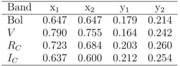
rors refer to one and one half spectral sub-classes.) An interpolation program by Terrell (1994, available from Nelson 2009) gave the Van Hamme (1993) limb darkening values; and finally, a logarithmic (LD = 2) law for the limb darkening coefficients was selected, appropriate for temperatures < 8500 K (ibid.). The limb darkening coefficients are listed in Table 3. (The values for the second star are based on the later-determined temperature of 5880 K and assumed spectral type of G1.) Convective envelopes for both stars were used, appropriate for cooler stars (hence values gravity exponent g = 0.32 and albedo A = 0.500 were used for each).

Figure 2. Broadening function at phase 0.285–smoothed and unsmoothed.

(5)

Table 3: Limb darkening values from Van Hamme (1993). Band x1 x2 y1 y2 Bol 0.647 0.647 0.179 0.214 V 0.790 0.755 0.164 0.242 RC 0.723 0.684 0.203 0.260 IC 0.637 0.600 0.212 0.254

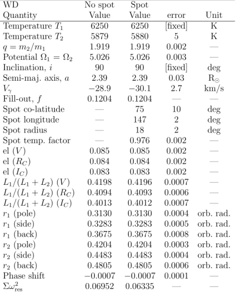
From the GCVS 4 designation (EW) and from the shape of the light curve, mode 3 (contact binary) mode was used. Early on, it was noted that the maxima between eclipses were slightly unequal. This is the O’Connell effect (Davidge & Milone 1984, and references therein) and is usually explained by the presence of one or more star spots. Because of the only slight difference between Max I (phase 0.25) and Max II (phase 0.75), a solution was first sought with no spots; later on, one was added first to star 2, and then to star 1. The latter gave better results and was adopted. In any case, the spotted solution gave only a marginal improvement in the fit. However, both unspotted and spotted solutions are presented in Table 4, even though the values are identical in most cases.

Convergence by the method of multiple subsets was reached in a small number of iter-ations. (The subsets were: (a, i, Ω1, L1), (i, T2, q), and (Vγ, i, Ω1). Almost immediately,

it was realized that a solution was impossible without third light (el3). Therefore third

light was added to the preliminary fitting, and that parameter was added to the third subset. Also, only values of the inclination near 90◦

were possible, with 90◦

always giving the best fit. In view of the fact that differential corrections always suggested non-physical corrections, the inclination was not varied thereafter.

Detailed reflections were tried, with nref = 1-3, but there was little—if any—difference

in the fit from the simple treatment. There are certain uncertainties in the process (see Csizmadia et al. 2013, Kurucz 2000). On the other hand, the solution is very weakly dependent on the exact values used.

In the first set of iterations (i.e., with no spot), when a fit was near, the sigmas for each dataset were adjusted, based on the output of WD (viz. computed from the sum of residuals for each dataset plus number of points).

The model is presented in Table 4. For the most part, the error estimates are those provided by the WD routines and are known to be low; however, it is a common practice to quote these values and we do so now. Also, estimating the uncertainties in temperatures T1 and T2 is somewhat problematic. A common practice is to quote the temperature

dif-ference over—say—one and one half spectral sub-classes (assuming that the classification is good to one or two spectral sub-classes, the precision being unknown). In addition, various different calibrations have been made (Cox 2000, page 388–390 and references therein, and Flower 1996), and the variations between the various calibrations can be significant. If the classification is ± one sub-class, an uncertainty of ± 200 K to the absolute temperatures of each, would be reasonable. (The modelling error in temperature T2, relative to T1, is indicated by the WD output to be much smaller, around 5 K.)

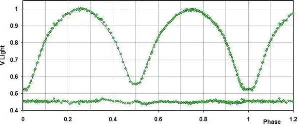
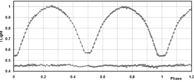
The light curve data and the fitted curves are depicted in Figures 4-6. The residuals (in the sense observed-calculated) are also plotted, shifted upwards by 0.45 units.

The radial velocities are shown in Fig. 7. A three-dimensional representation from Binary Maker 3 (Bradstreet 1993) is shown in Fig. 8.

(6)

IBVS6192 ₅

Table 4: Wilson-Devinney parameters.

WD No spot Spot

Quantity Value Value error Unit Temperature T1 6250 6250 [fixed] K

Temperature T2 5879 5880 5 K

q = m2/m1 1.919 1.919 0.002 —

Potential Ω1 = Ω2 5.026 5.026 0.003 —

Inclination, i 90 90 [fixed] deg Semi-maj. axis, a 2.39 2.39 0.03 R⊙

Vγ −28.9 −30.1 2.7 km/s

Fill-out, f 0.1204 0.1204 — — Spot co-latitude — 75 10 deg Spot longitude — 147 2 deg

Spot radius — 18 2 deg

Spot temp. factor — 0.976 0.002 — el (V ) 0.085 0.085 0.002 — el (RC) 0.084 0.084 0.002 — el (IC) 0.083 0.083 0.002 — L1/(L1+ L2) (V ) 0.4198 0.4196 0.0007 — L1/(L1+ L2) (RC) 0.4094 0.4093 0.0006 — L1/(L1+ L2) (IC) 0.4013 0.4012 0.0007 —

r1 (pole) 0.3130 0.3130 0.0004 orb. rad.

r1 (side) 0.3283 0.3283 0.0005 orb. rad.

r1 (back) 0.3675 0.3675 0.0008 orb. rad.

r2 (pole) 0.4204 0.4204 0.0003 orb. rad.

r2 (side) 0.4483 0.4483 0.0004 orb. rad.

r2 (back) 0.4805 0.4805 0.0006 orb. rad.

Phase shift −0.0007 −0.0007 0.0001 — Σω2

res 0.06952 0.06335 — —

The WD output fundamental parameters and errors are listed in Table 5. Correspond-ing values from the spotted and unspotted solutions agreed within the displayed digits in all cases, so therefore only one set of values is given. Most of the errors are output or derived estimates from the WD routines. From Kallrath & Milone (1998), the fill-out factor is f = (ΩI− Ω)/(ΩI− ΩO), where Ω is the modified Kopal potential of the system,

ΩI is that of the inner Lagrangian surface, and ΩO, that of the outer Lagrangian surface,

was also calculated.

To determine the distance r, the analysis proceeded as follows: first the WD routine gave the absolute bolometric magnitudes of each component; these were then converted to the absolute visual (V ) magnitudes of both, MV,1 and MV,2, using the bolometric

corrections BC = –0.160 and –0.190 for stars 1 and 2 respectively. The latter were taken from interpolated tables constructed from Cox (2000). The absolute V magnitude was then computed in the usual way, getting MV = 4.14 ± 0.03 magnitudes. The apparent

magnitude in the V passband was V = 10.00 ± 0.03, taken from the Tycho values (Hog, et al., 2000) and converted to a Johnson magnitude using relations due to Henden (2001). The colour excess (in B − V ) was obtained in the usual way, by subtracting the tabular value of B − V (for that spectral class) from the observed (converted Tycho) value. This

(7)

gave E[B − V ] = 0.18 magnitudes. However, reference to the dust tables of Schlegel et al. (1998) revealed a value of E[B − V ] = 0.2823 for those galactic coordinates. Since the E[B −V ] values have been derived from full-sky far-infrared measurements, they therefore apply to objects outside of the Galaxy; this value of E[B − V ] so derived then represents an upper limit for closer objects within the Galaxy. Hence the lower value of 0.18 is reasonable, and was adopted. (An uncertainty of—say—half this amount was used in the error calculation for distance.)

Figure 4. V light curves for V2477 Cyg – data, WD fit, and residuals.

Figure 5. RC light curves for V2477 Cyg – data, WD fit, and residuals.

Galactic extinction was obtained from the usual relation AV = RE[B − V ], using

R = 3.1 for the reddening coefficient. Hence, distance r = 112 pc was calculated from the standard relation:

r = 100.2(V −MV−AV+5)

(8)

IBVS6192 ₇

Figure 6. IC light curves for V2477 Cyg – data, WD fit, and residuals.

Figure 7. Radial velocity curves for V2477 Cyg – data and WD fit.

(9)

Table 5: Fundamental parameters.

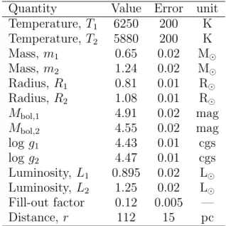
Quantity Value Error unit Temperature, T1 6250 200 K Temperature, T2 5880 200 K Mass, m1 0.65 0.02 M⊙ Mass, m2 1.24 0.02 M⊙ Radius, R1 0.81 0.01 R⊙ Radius, R2 1.08 0.01 R⊙ Mbol,1 4.91 0.02 mag Mbol,2 4.55 0.02 mag log g1 4.43 0.01 cgs log g2 4.47 0.01 cgs Luminosity, L1 0.895 0.02 L⊙ Luminosity, L2 1.25 0.02 L⊙ Fill-out factor 0.12 0.005 — Distance, r 112 15 pc

The errors were assigned as follows: δMbol,1 = δMbol,2 = 0.014, δBC1 = δBC2 = 0.015

(the variation of 1.5 spectral sub-classes), δV = 0.03, δE(B–V ) = 0.07, all in magnitudes, and δR = 0.1. Combining the errors rigorously (i.e., by adding the variances) yielded an estimated error in r of 15 pc.

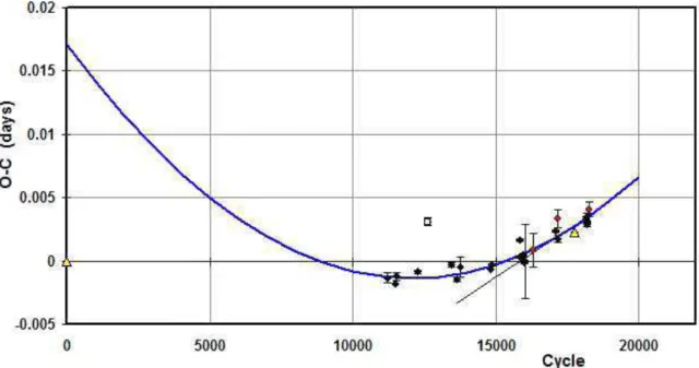
Some comments regarding the period variation are in order. An eclipse timing differ-ence (O − C) plot is depicted in Fig. 9. It will be seen that even though the existing points, almost all derived using CCD detectors, display considerable scatter, it is still possible to fit a quadratic relation. (Notes: for determining the elements of equation 1, a tangent line was used, and the open square represents a rejected datum.) But what should one do with the original point from 1999 (at cycle 0)?

Rucinski et al. (2007 and references therein) showed that, for close binaries, a third component is very common. So therefore the light time effect (LiTE) (whereby the orbit-ing pair makes an orbit about the common centre of mass, and the light information may be advanced or retarded due to varying distance to the observer), may play a role in the period variation. Irwin (1952, 1959) provided the equations for computing the theoretical period variation, based on the period of the third star, P3 and other orbital parameters.

Using these equations, it is possible to fit not one but many (at least seven) different LiTE relations to all the points using periods P3 ranging from 14 to 35 years. It is obvious that no definitive solution for the orbital parameters of the putative third star orbit will be possible without many new points spanning perhaps a decade or more. However the point is that it is at least plausible that the light time effect exists and that the point at 0,0 is not aberrant. The O − C file may be found online at Nelson (2016).

In conclusion, the fundamental parameters of this system have been determined. It has been shown to have a low degree of contact, expressed by the fill-out parameter f = 0.120. This is typical for a W-type contact binary (Rucinski 1974). Also, the existence a significant third light is consistent with the high proportion of contact binaries having a third component (Rucinski 2007, and references therein).

(10)

IBVS6192 ₉

Figure 9. V2477 Cyg – eclipse timing (O − C) diagram with a quadratic fit for points after cycle 10000.

No evidence of the third star was seen in the spectra. This is hardly surprising because of the relatively weak contribution from the third light. Because the relative flux at phases 0.25 and 0.75 has been normalized to close to unity, quantity l3 represents the fractional

contribution to the flux there (Wilson 1998, page 5). Assuming isotropic radiation from the third star, then its luminosity may be estimated by el3×(total luminosity of system) =

0.04 × 2.1 = 0.08. If the companion is a main sequence star, this would make it a red dwarf of spectral type M1–M2—far too faint to register in the spectra above the noise.

It is somewhat troubling that the spectroscopic mass ratio qsp = 2.17(2) differs

signifi-cantly from that derived by the light curve modelling, qptm = 1.919(2). In view of the fact

that the eclipses are total, we may trust the photometric value (Terrell & Wilson 2005). Moreover, the excellent fit of theoretical to observed light curves (Figs. 4-6) gives one confidence in the photometric value. But why is the spectroscopic value deviant?

It is tempting to believe that more spectra would clarify the situation, but there is much to be said for these spectra: they have a high signal-to-noise ratio, with continuum levels ranging from 20,000 to over 50,000; unlike some cases, the spectra reproduced in Fig. 1 display highly significant shifts over phase; the broadening functions, as reproduced in Figs. 2 and 3, are robust, with low noise and little to compromise the RV extraction; and finally, all estimates for the RV errors lie somewhat less than 10 km/s, typical in this work.

Although it has been argued that the contribution from the third star is low, it seems possible that its light has contaminated the spectra, distorting the RV determination.

Whatever the cause of the disparity, it seems safe to assume that the photometric mass ratio is more reliable and that the derived fundamental parameters are reliable.

Acknowledgements: It is a pleasure to thank the staff members at the DAO (especially Dmitry Monin and David Bohlender) for their usual splendid help and assistance.

(11)

References:

Bradstreet, D.H., 1993, “Binary Maker 2.0 - An Interactive Graphical Tool for Preliminary Light Curve Analysis”, in Milone, E.F. (ed.) Light Curve Modelling of Eclipsing Binary Stars, pp 151-166 (Springer, New York, N.Y.)

Cox, A.N., ed, 2000, Allen’s Astrophysical Quantities, 4th ed., (Springer, New York, NY) Csizmadia, S., Pasternacki, T., Dreyer, C., Cabrera, A., Erikson, A., Rauer, H., 2013,

A&A, 549, A9 DOI

Davidge, T.J., Milone, E.F., 1984, ApJS, 55, 571 DOI Flower, P.J., 1996, ApJ, 469, 355 DOI

Gessner, H., 1966, Ver¨off. Sternwarte Sonneberg, 7, 61

Henden, A., 2001, http://www.tass-survey.org/tass/catalogs/tycho.old.html Hoffmeister, C. von, 1963, AN, 287, 169 DOI

Hog, E., et al., 2000, A&A, 355, L27 Irwin, J.B., 1952, ApJ, 116, 211 DOI Irwin, J.B., 1959, AJ, 64, 149 DOI

Kallrath, J., Milone, E.F., 1998, Eclipsing Binary Stars–Modeling and Analysis (Springer-Verlag) DOI

Kallrath, J., Milone, E.F., Terrell, D., Young, A.T., 1998, ApJ, 508, 308 DOI Kurucz, R.L., 2000, Baltic Astron., 11, 101

Nelson, R.H., 2009, software by Bob Nelson,

http://members.shaw.ca/bob.nelson/software1.htm Nelson, R.H., 2010a, spreadsheets by Bob Nelson,

http://members.shaw.ca/bob.nelson/spreadsheets1.htm

Nelson, R.H., 2010b, “Spectroscopy for Eclipsing Binary Analysis” in The Alt-Az Initia-tive, Telescope Mirror & Instrument Developments (Collins Foundation Press, Santa Margarita, CA), R.M. Genet, J.M. Johnson and V. Wallen (eds)

Nelson, R.H., 2016, Bob Nelson’s O−C Files, http://www.aavso.org/bob-nelsons-o-c-files Nelson, R. H., S¸enavcı, H.V. Ba¸st¨urk, ¨O., Bahar, E., 2014, New Astron., 29, 57 DOI

Otero, S.A., Wils, P., 2005, IBVS, 5630 Rucinski, S. M., 1974, AcA, 24, 119 Rucinski, S. M., 2004, IAUS, 215, 17

Rucinski, S. M., Pribulla, T., and van Kerkwijk, M.H., 2007, AJ, 134, 2353 DOI Schlegel, D.J., Finkbeiner, D.P., Davis, M., 1998, ApJ, 500, 525 DOI

Skiff, B.A., 1999, IBVS, 4720

Terrell, D., 1994, Van Hamme Limb Darkening Tables, vers. 1.1. Terrell, D. Wilson, R.E., 2005, ApSS, 296, 221 DOI

Van Hamme, W., 1993, AJ, 106, 2096 DOI

Wilson, R.E., Devinney, E.J., 1971, ApJ, 166, 605 DOI Wilson, R.E., 1990, ApJ, 356, 613 DOI

Wilson, R.E., 1998, Documentation of Eclipsing Binary Computer Model (available from the author)