Algorithms for uniform optimal strategies in two-player zero-sum stochastic games with perfect information

HAL Id: inria-00506390

https://hal.inria.fr/inria-00506390

Submitted on 27 Jul 2010

HAL is a multi-disciplinary open access

archive for the deposit and dissemination of

sci-entific research documents, whether they are

pub-lished or not. The documents may come from

L’archive ouverte pluridisciplinaire HAL, est

destinée au dépôt et à la diffusion de documents

scientifiques de niveau recherche, publiés ou non,

émanant des établissements d’enseignement et de

zero-sum stochastic games with perfect information

Konstantin Avrachenkov, Laura Cottatellucci, Lorenzo Maggi

To cite this version:

Konstantin Avrachenkov, Laura Cottatellucci, Lorenzo Maggi. Algorithms for uniform optimal

strate-gies in two-player zero-sum stochastic games with perfect information. [Research Report] RR-7355,

INRIA. 2010. �inria-00506390�

a p p o r t

d e r e c h e r c h e

Algorithms for uniform optimal strategies in

two-player zero-sum stochastic games with perfect

information

Konstantin Avrachenkov — Laura Cottatellucci — Lorenzo Maggi

N° 7355

Konstantin Avrachenkov

, Laura Cottatellucci

, Lorenzo Maggi

Thème COM — Systèmes communicants Projet Maestro

Rapport de recherche n° 7355 — July 2010 — 22 pages

Abstract: In stochastic games with perfect information, in each state at most one player has more

than one action available. We propose two algorithms which find the uniform optimal strategies for zero-sum two-player stochastic games with perfect information. Such strategies are optimal for the long term average criterion as well. We prove the convergence for one algorithm, which presents a higher complexity than the other one, for which we provide numerical analysis.

Key-words: Stochastic games, Perfect information, Uniform optimal strategies, Computation

∗_{INRIA Sophia Antipolis-Méditerranée, France, k.avrachenkov@sophia.inria.fr}

†_{Eurecom, Mobile Communnications, France, laura.cottatellucci@eurecom.fr} ‡_{Eurecom, Mobile Communnications, France, lorenzo.maggi@eurecom.fr}

joueurs et avec information parfaite

Résumé : Dans les jeux stochastiques à information parfaite, dans chaque etat, au plus, un joueur a plus d’une action disponibles. Nous proposons deux algorithmes qui trouvent les stratégies uniformément optimales pour les jeux stochastiques à somme nulle avec deux joueurs et information parfaite. Ces stratégies sont aussi optimales pour le critère de la moyenne à long terme. Nous prouvons la convergence pour un algorithme, qui a une plus grande complexité que l’autre, pour lequel nous offrons une analyse numérique.

1

Introduction

Stochastic games are multi-stage interactions among several participants in an environment whose conditions change stochastically, influenced by the decisions of the players. Such games were in-troduced by Shapley (1953), who proved the existence of the discounted value and of the stationary discounted optimal strategies in two-player zero-sum games with finite state and action spaces. The problem of long term average reward games was addressed first by Gillette (1957). Bewley and Kohlberg (1976) proved that the field of real Puiseux series is an appropriate class to study the asymptotic behavior of discounted stochastic game when the discount factor tends to one. Mertens and Neyman (1981) showed the existence of the long term average value of stochastic games. Then, Parthasarathy and Raghavan (1981) first introduced the notion of order field property. This prop-erty implies that the solution of a game lies in the same ordered field of the game data. Solan and Vieille (2009) presented an algorithm to find theε-optimal uniform discounted strategies in two-player zero-sum stochastic games, whereε> 0.

Perfect information games were addressed by several researchers (e.g. see Thuijsman and Ragha-van, 1997, Altman and Feinberg, 2000), since they are the most elementary form of stochastic games: the reward and the transition probabilities in each state are controlled at most by one player. Recently, Raghavan and Syed (2002) provided an algorithm which finds the optimal strategies for two-player zero-sum perfect information games under the discounted criterion for a fixed discount factor.

Markov Decision Processes (MDPs) can be seen as stochastic games in which only one player can possess more than one action in each state. It is well known (see e.g. Filar and Vrieze, 1996) that the optimal strategy in an MDP can be computed with the help of a linear programming for-mulation. Hordijk, Dekker and Kallenberg (1985) proposed to find the Blackwell optimal strategies (uniform optimal discount strategies) for MDPs by using the simplex method in the ordered field of rational functions with real coefficients. Altman, Avrachenkov and Filar (1999) analysed singularly perturbed MDP using the simplex method in the ordered field of rational functions. More generally, Eaves and Rothblum (1994) studied how to solve a vast class of linear problems, including linear programming, in any ordered field.

In this paper we propose two algorithms to determine the uniform optimal discount strategies in two-player zero-sum games with perfect information. Such strategies are optimal in the long run average criterion as well. The proposed approaches generalize the works by Hordijk, Dekker,

Kallenberg (1985) and Raghavan, Syed (2003) to the game model in the field F(R) of the

non-archimedean ordered field of rational functions with coefficients inR.

LetΓbe a two-player zero-sum stochastic game with perfect information andΓi(h), i = 1, 2 be the MDP that player i faces when the other player fixes his own strategy h. Our first algorithm can be summed up in the following 3 steps:

1. Choose a stationary pure strategy g for player 2.

3. Find the first state controlled by player 2 in which a change of strategy g′is a benefit for player 2 for all the discount factors close enough to 1. If it does not exists, then(f, g) are uniform

optimal, otherwise set g := g′_{and go to step 2.}

It is evident that player 1 is left totally free to optimize the MDP that he faces at each iteration of the algorithm in the most efficient way.

Our second algorithm is a best response approach, in which the two players alternatively find their own uniform optimal strategies:

1. Choose a stationary pure strategy g for player 2.

2. Find the uniform optimal strategy f for player 1 in the MDPΓ1(g).

3. If g is uniform optimal for player 2 in the MDPΓ2(f), then (f, g) are uniform optimal.

Other-wise, find the uniform optimal strategy g′inΓ2(f), set g := g′and go to step 2.

The convergence in a finite time of the first algorithm is proven, while for the second we provide numerical analysis. We also show that the second algorithm has a lower complexity.

This paper is organized as follows. In section 2 we introduce formally the properties of stochastic games, section 3 is dedicated to the description of the field of rational functions with real coefficients, while in section 4 we recall the linear programming procedures in the field F(R) in order to find a

Blackwell optimal policy for MDPs. We present some new useful results on perfect information games in section 5 and section 6 is dedicated to the description and to the validation of our first algorithm. In section 7 we provide a numerical example. In section 8 we introduce an algorithm whose convergence is only conjectured; we report some considerations and numerical results about the complexity of our algorithms in section 8.1.

Some notation remarks: the ordering relation between vectors of the same length a≥ (≤)b

means that for every component i, a(i) ≥ (≤)b(i). The discount factor and the interest rate are

barred (β,ρ) if they are a fixed value; the symbolsβ,ρrepresent the related variables.

2

The model

In a two-player stochastic gameΓwe have a set of states S= {s1, s2, . . . , sN}, and for each state s the set of actions available to the i-th player is called A(i)(s) = {a(i)₁ (s), . . . , a(i)_m

i(s)}, i = 1, 2. Each

triple(s, a1, a2) with a1∈ A(1), a2∈ A(2)is assigned an immediate reward r(s, a1, a2) for player 1, −r(s, a1, a2) for player 2 and a transition probability distribution p(.|s, a1, a2) on S.

A stationary strategy u∈ USfor the i-th player determines the probability u(a|s) that in state s player i chooses the actions a∈ [a(i)₁ , . . . , a(i)_m

i(s)].

It is evident that a couple of strategies f∈ FS, g ∈ GSfor player 1 and 2, respectively, sets up a Markov chain in which the transition probability equals

p(s′|s, f, g) = m1(s)

∑

∑

∀ s, s′_{∈ S, while the average immediate reward r(s, f, g) equals}

r(s, f, g) = m1(s)

∑

∑

Letβ ∈ [0; 1) be the discount factor and ρ be the interest rate such thatβ(1 +ρ) = 1. Note

that whenβ ↑ 1, thenρ ↓ 0. We defineΦ_β(f, g) as a column vector of length N such that its i-th

component equals the expectedβ-discounted reward when the initial state of the stochastic game is

si: Φ_β(f, g) = ∞

∑

where P(f, g) and r(f, g) are the N-by-N transition probability matrix and the N-by-1 average reward

vector associated to the couple of strategies(f, g) respectively.

Definition 1. Theβ-discounted value of the gameΓis such that

Φ_β(Γ) = sup f

inf

g Φβ(f, g) = infg sup_f Φβ(f, g). (1)

Definition 2. An optimal strategy f∗_β for player 1 assures to him a reward which is at leastΦ_β(Γ)

Φ_β(f∗_β, g) ≥Φ_β(Γ) ∀ g ∈ G

while g∗_β is optimal for player 2 iff

Φ_β(f, g∗_β) ≤Φ_β(Γ) ∀ f ∈ F.

LetΦ(f, g) be the long term average value of the gameΓassociated to the couple of strategies

(f, g): Φ(f, g) = lim T→∞ 1 T+ 1 T

∑

andΦ(Γ) be the value vector for the long term average criterion of the gameΓ, defined in an analo-gous way to expression (1).

The existence of optimal strategies in discounted stochastic games is guaranteed by the following theorem (Filar and Vrieze, 1996):

Theorem 2.1. Under the hypothesis of discounted pay-off, stochastic games possess a value, the

optimal strategies(f∗

β, g∗β) exist among stationary strategies and moreoverΦβ(Γ) =Φβ(f∗β, g∗β).

Definition 3. A stationary strategy h is said to be uniformly discount optimal for a player if h is

optimal for everyβ close enough to 1 (or, equivalently, for allρclose enough to 0).

In the present paper we deal with perfect information stochastic games.

Definition 4. Under the hypothesis of perfect information, in each state at most one player has more

than one action available.

Let S1= {s1, . . . , st1} be the set of states controlled by player 1 and S2= {st1+1, . . . , st1+t2} be

the set controlled by player 2, with t1+t2≤ N.

3

The ordered field of rational functions with real coefficients

Let P(R) be the ring of all the polynomials with real coefficients.

Definition 5. The dominating coefficient of a polynomial f = a0+ a1x+ · · · + anxnis the coefficient

ak, where k= min{i : ai6= 0} and we denote it with D( f ).

Let F(R) be the non-archimedean ordered field of fractions of polynomials with coefficients in R:

f(x) = c0+ c1x+ · · · + cnx

n

d0+ d1x+ · · · + dmxm

f ∈ F(R)

where the operations of sum and product are defined in the usual way (see Hordijk, Dekker and Kallenberg, 1985). Two rational functions h/g, p/q are identical (and we say h/g =l p/q) if and only if h(x)q(x) = p(x)g(x) ∀x ∈ R.

The following lemma (Hordijk et al., 1985) introduces the ordering in the field F(R):

Lemma 3.1. A complete ordering in F(R) is obtained by the rule

p

q >l0 ⇐⇒ D(p)D(q) > 0 p, q ∈ P(R)

In the same way, we can also define the operations of maximum (max_l) and minimum (min_l) in

F(R).

The ordering law defined above is useful when one wants to compare the behavior of rational functions whose indipendent variable is positive and approaches to 0 (see Hordijk et al., 1985).

Lemma 3.2. The rational function p/q is positive (p/q >l0) if and only if there exists x0> 0 such

3.1

Application to stochastic games

From the next theorems the reader will start perceiving the importance of dealing with the field F(R)

in stochastic games.

Theorem 3.3. Let f, g be two stationary strategies respectively for players 1 and 2 andΦρ(f, g) : R → RN_{be the discounted reward associated to the couple of strategies(f,g) expressed as a variable}

ofρ. Then,Φ_ρ(f, g) ∈ F(R).

Proof. For any couple of stationary strategies(f, g), we can write

N

∑

s′=1

[(1 +ρ)δs,s′− p(s′|s, f, g)]Φ_ρ(f, g, s′) = (1 +ρ)r(s, f, g) s ∈ [1; N] (2)

whereρis a variable. By solving the above system of equations in the unknownΦ_ρby Cramer rule, it is evident thatΦ_ρ(f, g) ∈ F(R).

Generally, the discounted value of a stochastic game for all the interest rates close enough to 0 belongs to the field of real Puiseux series (see Filar and Vrieze, 1996). From Theorems 2.1 and 3.3 it is straightforward to obtain the following important Lemma.

Lemma 3.4. LetΓbe a zero-sum stochastic game which possesses uniform discount optimal strate-gies for both players. Then, there existρ∗> 0 andΦ∗_ρ(Γ) ∈ F(R) such thatΦ∗_ρ(Γ) is the discounted

optimal value for all the interest ratesρ∈ (0;ρ∗].

Proof. Let(f∗_{, g}∗_{) be a couple of uniformly discount optimal strategies for players 1 and 2}

respec-tively. Then, by definition, there existsρ∗> 0 such that (f∗_{, g}∗_{) are discounted optimal for all the}

interest ratesρ∈ (0;ρ∗]. From Theorem 3.3 we know thatΦρ(f∗_{, g}∗_{) ∈ F(R) and, from Theorem}

2.1, the optimum uniform discounted valueΦ_ρ(Γ) =Φρ(f∗_{, g}∗_{) ∀ρ∈ (0;ρ}∗_{]. So,Φ}∗

ρ(Γ) ∈ F(R) represents the discounted value ofΓfor all the interest rates sufficiently close to 0.

Lemma 3.5. LetΓbe a zero-sum stochastic game which possesses uniform discount optimal strate-gies f∗, g∗for players 1 and 2 respectively. Then,

Φρ(f, g∗) ≤lΦρ(f∗, g∗) =lΦ∗ρ(Γ) ≤lΦρ(f∗, g) ∀ f, g (3) where Φ∗ ρ(Γ) =lmaxl f min_l g Φρ(f, g) =lminl g max_l f Φρ(f, g). (4)

Proof. From Theorem 2.1 and by the definition of uniform discount optimal strategy, we assert that

∃ρ∗> 0 : ∀ρ∈ (0;ρ∗] ⇒ Φρ(f, g∗) ≤Φρ(f∗, g∗) ≤Φρ(f∗, g) ∀ f, g

which coincides with (3) for Lemma 3.2. The equation (4) is a direct consequence of (3).

4

Computation of Blackwell optimum policy in MDPs

In this section we will discuss about some concepts of linear programming, which can be easily found on any book on linear optimization (e.g. see Luenberger and Ye 2008).

Let Ψbe a Markov Decision Process, which can be seen as a two-player stochastic game in

which one of the two players either fixes his own strategy or has only one available action in each state. We callΦ_ρ(f) the value of the discounted MDP associated to the strategy f with interest rate

variableρ.

It is known (Puterman, 1994) that the interval of interest rate(0;∞) can be broken into a finite

number n of subintervals, say(0 ≡α0;α1], (α1;α2], . . . , (αn−1;∞) in such a way that for each one

there exists an optimal pure strategy.

A Blackwell optimal policy is an optimal strategy associated to the first sub-interval.

Definition 7. We say that the strategy f∗is Blackwell optimal iff there exists ¯ρ∗> 0 such that f∗_is

optimal in the(1/ ¯ρ− 1)-discounted MDP for all the interest rates ¯ρ∈ (0; ¯ρ∗_].

Since for Theorem 3.3Φ_ρ(f) ∈ F(R) for any f ∈FS, we can say

Φρ(f∗) ≥lΦρ(f) ∀ f ∈ F where F is the set of all possible strategies.

Hordijk, Dekker and Kallenberg (1985) provided a useful algorithm to compute the Blackwell opti-mum policy in MDPs. It consists in solving the following parametric linear programming problem:

     max x l∑ N s=1∑ m(s) a=1xsa(ρ)r(s, a) ∑N s=1∑ m(s) a=1[(1 +ρ)δs,s′− p(s′|s, a)] x_s,a(ρ) =_l1, s′∈ S xs,a(ρ) ≥l0, s∈ S, a ∈ A(s) (5)

in the ordered field of rational functions with real coefficients F(R). This means that

i) ρis the variable of polynoms;

ii) all the elements of the related simplex tableau belong to F(R);

iii) all the algebraic and ordering operations required by the simplex method are carried out in the

field F(R).

The practical technique to solve the linear optimization problem (5) proposed by Hordijk et al. (1985) is the so-called two-phases method.

In the first phase the artificial variables z1, . . . , zNare introduced as basic variables and the tableau of the following linear programming problem

     max x _l∑ N s=1∑ m(s) a=1xsa(ρ)r(s, a) ∑N s=1∑ m(s) a=1[(1 +ρ)δs,s′− p(s′|s, a)] x_s,a(ρ) + z_s′(ρ) =_l1, s′∈ S xs,a(ρ) ≥l0, s∈ S, a ∈ A(s) (6)

is built. Then, N successive pivot operations on all the artificial variables are carried out so that the feasibility of the solution is preserved. We call entering variables the basic variables of the tableau at the end of the first phase. In the second phase the columns of the tableau associated to the artificial variables z1, . . . , zN(which are now all non-basic) are removed and the simplex method is performed in the ordered field F(R) on the obtained tableau.

We note that another approach for the solution of the parametric linear program (5) is given by simplex method in the field of Laurent series (see Filar, Altman and Avrachenkov, 2002).

The optimal Blackwell stationary pure strategy f∗is computed as:

f∗(a|s) = x ∗ s,a(ρ) ∑m(s) a=1x∗s,a(ρ) ∀ s ∈ S, a ∈ A(s) (7) where{x∗s,a(ρ) ∀ s, a} is the solution of the optimization problem. The simplex method guarantees

that the optimum strategy f∗is well-defined and pure (see Filar and Vrieze 1996).

5

Uniform optimality in perfect information games

As we said before, in a perfect information game in each state at most one player has more than one action available. A stationary strategy for the player i= 1, 2 is a function fi : S→SNk=1Ai(sk) with

fi(.|st) ∈ Ai(st).

Theorem 5.1. For a stochastic game with perfect information, both players possess uniform

dis-count optimal pure stationary strategies, which are optimal for the average criterion as well.

The Theorem 5.1 (see Filar and Vrieze, 1996) guarantees the existence of the optimal strategies for both players in the average criterion for games with perfect information. Moreover, it suggests that in order to find the optimal strategies for the average criterion one has to find the optimal strate-gies in the discounted criterion for a discount factor sufficiently close to 1.

Definition 8. We call two pure stationary strategies adjacent if and only if they differ only in one

state.

Then the following property holds, which proof is analogous to the one in the field of real num-bers.

Lemma 5.2. Let g be a strategy for player 2 and f, f1be two adjacent strategies for player 1. Then

eitherΦ_ρ(f1, g) ≥lΦρ(f, g) orΦρ(f1, g) ≤lΦρ(f, g), which means that the two vectors are partially

ordered.

The property above allows us to give the following definition.

Definition 9. Let(f, g) be a pair of pure stationary strategy respectively for player 1 and 2. We call

f1(g1) a uniform adjacent improvement for player 1 (2) in state st if and only if f1(g1) is a pure

stationary strategy which differs from f(g) only in state st andΦρ(f1, g) ≥lΦρ(f, g) (Φρ(f, g1) ≤l

As in the case in which the discount interest rate is fixed, we achieve the following results.

Lemma 5.3. LetΓbe a perfect information stochastic game. A couple of pure stationary strategies

(f∗, g∗) is uniform discount optimal if and only if no uniform adjacent improvement is possible for

both players.

Proof. The only if implication is obvious. If the strategies(f∗, g∗) are such that no uniform adjacent

improvements are possible for both players, then no improvements are possible also for the first stage of the game too, that is

f∗(s) = argmax l a∈A1(s) ( r(s, a) + (1 +ρ)−1 N

∑

∑

It is known (see Filar and Vrieze, 1996) that if the strategies(f∗, g∗) satisfy such equations then they

are uniform discount optimal.

In perfect information games, the following result (see Raghavan and Syed, 2002) holds

Lemma 5.4. In a zero-sum, perfect information, two-player discounted stochastic gameΓ with interest rateρ> 0, a pair of pure stationary strategies (f∗, g∗) is optimal if and only ifΦρ(f∗, g∗) =

Φρ(Γ), the value of the discounted stochastic gameΓ.

From the above result we can easily derive the analogous property in the ordered field F(R).

Lemma 5.5. In a zero-sum, two-player stochastic gameΓwith perfect information, a pair of pure stationary strategies(f∗_{, g}∗_{) are uniform discount optimal if and only ifΦρ(f}∗_{, g}∗_{) =}

lΦ∗_ρ(Γ) ∈ F(R),

whereΦ∗_ρ(Γ) is the uniform discount value ofΓ.

Proof. The only if statement coincides with the assertion of Theorem 2.1. The if condition is less

obvious. If a pair of strategies(f∗_{, g}∗_{) has the propertyΦρ(f}∗_{, g}∗_{) =}

lΦ∗_ρ(Γ), then there existsρ∗> 0 such that ∀ρ ∈ (0;ρ∗_{], Φ}

ρ(f∗, g∗) coincides with the value of the game Γ, ∀ρ ∈ (0;ρ∗]. Then, thanks to Lemma 5.4, we can say that∀ρ∈ (0;ρ∗_{] the strategies f}∗_{, g}∗_{are optimal in the discounted}

gameΓ, which means that they are discount optimal.

Let st be a state controlled by player i (i= 1, 2) and X ⊂ Ai(st). Let us callΓt_X the stochastic game which is equivalent toΓexcept in state st, where player i has only the actions X available. Analogously to the result of Raghavan and Syed (2002), we propose the following Lemma.

Lemma 5.6. Let i= 1, 2 and st ∈ Si, X⊂ Ai(st), Y ⊂ Ai(st), X ∩ Y = /0. ThenΦ∗ρ(ΓtX∪Y) ∈ F(R),

which is the uniform value of the gameΓt_X∪Y, equals

Φ∗ ρ(ΓtX∪Y) = maxl{Φ ∗ ρ(ΓtX),Φ∗ρ(ΓtY)} if i= 1 Φ∗ ρ(ΓtX∪Y) = minl{Φ ∗ ρ(ΓtX),Φ∗ρ(ΓtY)} if i= 2.

Proof. Let us suppose that the state st is controlled by player 2. We indicate with GtX the set of pure stationary strategies in which the choice in state st is restricted to the set X . We note that the restriction in state stdoes not affect player 1. Thus, FtX= F.

If it is possible to find optimal strategies for player 2 both in Gt_X and in Gt_Y, then Φ∗_ρ(Γt

X) =l

Φ∗

ρ(ΓtY) =lΦ∗_ρ(ΓtX∪Y) for Lemma 5.5.

Otherwise, the uniform discount pure strategy of gameΓt_X∪Y for player 2 belongs either to Gt_Xor to

Gt_Y. For example, let us suppose that the optimal discount strategy in the stochastic gameΓt_X∪Y for player 2 is found in Y . Then we have

Φ∗ ρ(ΓtY) =lΦ∗ρ(ΓtX∪Y) =lminl g∈G max_l f∈F Φρ(f, g) ≤lminl g∈Gt X max_l f∈F Φρ(f, g) =lΦ∗ρ(ΓtX)

The proof for the situation in which st∈ S1is analogous.

6

Algorithm description

Our task is to find an algorithm which allows to find the uniform discount optimal strategies for both players in a perfect information stochastic gameΓ, which coincide with the optimal strategies for the long term average criterion for Theorem 5.1. Following the lines of the algorithm of Raghavan and Syed (2002) for optimal discount strategy, we propose an algorithm suitable to the ordered field

F(R).

LetΓbe a zero-sum two-player stochastic game with perfect information.

Note that all the algebraic operations and the order signs (<, >) are to be intended in the field

F(R).

Remark 1. Unlike Raghavan and Syed’s solution, the algorithm ?? does not require the strategy

search for player 1 to be lexicographic. Player 1, in fact, faces in step 2 a classic Blackwell opti-mization.

Remark 2. Obviously, the roles of player 1 and 2 can be swapped in the algorithm ??. For simplicity,

throughout the paper the player 1 will be assigned to step 2.

Remark 3. In step 3, once the state st1+kis found, the adjacent improvement involves the pivoting of any of the non basic variable xs_t1+k,ato which corresponds a reduced cost cs_t1+k,a≤l0.

Now, we prove the appropriateness of the algorithm ??. The proof is analogous to the one by Raghavan and Syed (2002).

Step 1 Choose randomly a stationary deterministic pure strategy g for player 2.

Step 2 Find the Blackwell optimal strategy for player 1 in the MDPΓ1(g) by solving within the field

F(R) the following linear programming:      max x l∑ N s=1∑ m1(s) a=1 xs,a(ρ)r(s, a, g) ∑N s=1∑ m1(s) a=1 [(1 +ρ)δs,s′− p(s′|s, a, g)] xs,a(ρ) =l1, s′∈ S xs,a(ρ) ≥l0, s∈ S, a ∈ A1(s) (8)

and compute the pure strategy f as

f(a|s) = x ∗ s,a(ρ) ∑m1(s) a=1 x∗s,a(ρ) ∀ s ∈ S, a ∈ A1(s) (9) where{x∗ s,a(ρ), ∀s, a} is the solution of (8).

Step 3 Find the minimum k such that in st1+k∈ {st1+1, . . . , st1+t2} there exists an adjacent

improve-ment g′ for player 2, with the help of the simplex tableau associated to the following linear programming:      max x l−∑ N s=1∑ m2(s) a=1 xs,a(ρ)r(s, f, a) ∑N s=1∑ m2(s) a=1 [(1 +ρ)δs,s′− p(s′|s, f, a)] xs,a(ρ) =l1, s′∈ S xs,a(ρ) ≥l0, s∈ S, a ∈ A2(s) (10)

where the entering variables are{xs,a: g(a|s) = 1, ∀s}.

If no such improvement for player 2 is possible then go to step 4, otherwise set g := g′_{and go}

to step 2.

Step 4 Set(f∗, g∗):=(f, g) and stop. The strategies (f∗, g∗) are uniform discount and long term average

optimal in the stochastic gameΓrespectively for player 1 and player 2.

Theorem 6.1. The algorithm stops in a finite time and the couple of strategies(f∗_{, g}∗_{) are uniform}

discount optimal in the stochastic gameΓ.

Proof. We assume that the overall number of actions

µ= t1

∑

∑

Without loss of generality, let us reorder the states so that in the first t1states player 1 has more than

one action and the second t2states are controlled by player 2. Of course, t1+t2≤ N.

We can proceed by induction onµ. Triviallyµ≥2N, becauseµ=2N is equivalent to the situation

t1= t2= 0. In this case the algorithm finds the average optimal couple of strategies because it is the

only existing.

Now we suppose by induction that the algorithm finds without cycling (that is, all pure stationary strategies are visited at most once) the couple of uniform optimal strategies when the number of actions isµ≥ 2N. We have to prove that the thesis is valid when the number of actions equalsµ+1.

If t2= 0, then again there is nothing to prove, because, as we showed in section 4, the step 1 of

our algorithm finds the Blackwell optimal policy f∗for player 1 in the MDPΓ1(g).

If t2≥ 0, then we focus on the state st1+t2= sτ, which is the last examined by our algorithm.

The actions available in state s_τ are A2(sτ) ≡ X ∪ ai, where X= {a1. . . ai−1, ai+1. . . an} and n ≥ 2 by hypothesis. By induction hypothesis, we suppose that the algorithm finds the uniform discount optimal strategies for both players in the gameΓτ_Xwithout cycling. Since no uniform improvements are possible inΓτ_Xby definition of uniform optimal strategies, then the algorithm looks for an uniform adjacent improvement g′, where g′(ai|sτ) = 1. There are now two possibilities.

If the uniform optimal strategy g for player 2 found inΓt

Xis also optimal inΓ, then the algorithm terminates because still no adjacent improvements are possible for player 2 in st.

Otherwise, any uniform optimal strategy g∗ for player 2 inΓ includes the action a_τ and the

algorithm necessarily finds an adjacent improvement in state s_τ for Theorem 5.3 and it finds by

induction hypothesis the uniform discount optimal strategies in the gameΓt

an. So we have Φρ(Γ) =lmin l {Φρ(Γ t X),Φρ(Γtan)} =lΦρ(Γ t an)

where the second equality holds because otherwise the optimal strategies ofΓt_X would be uniform

optimal in the gameΓfor Lemma 5.5. Again thanks to Lemma 5.5, we can assert that the uniform

discount optimal strategies(f∗, g∗) found inΓt

an are optimal also forΓ, becauseΦρ(f

∗_{, g}∗_{) =Φ}∗

ρ(Γ),

which is the uniform discount value of the game.

Moreover, the algorithm terminates because for Theorem 5.3 no improvements are available to both players.

We gave a constructive proof of the fact that the algorithm passes through a path of pure strate-gies, it never cycles and it finds the uniform discount optimal strategies for both players. Since the

overall number of actions is finite, then also the cardinality of pure strategies is finite; hence, the algorithm must terminate in a finite time and the strategies(f∗_{, g}∗_{) are uniform discount optimal, and}

for Theorem 5.1 they are long term average optimal as well.

6.1

Computing the optimality range factor

The algorithm presented in section 6 suggests a way to determine the range of discount factor in which the long term average optimal strategies(f∗, g∗) are also optimal in the discounted game.

Before, we report the analogous result to Lemma 5.3 when the discount factor is fixed (see Raghavan and Syed, 2002).

Lemma 6.2. LetΓbe a perfect information stochastic game andβ∈ [0; 1). The pure stationary

strategies(f∗, g∗) areβ-discount optimal if and only if no uniform adjacent improvements are pos-sible for both players in theβ-discounted stochastic gameΓ.

Let us define withζ( fρ), where fρ∈F(R), the set of positive roots of fρsuch thatd f_dρρρ=u< 0 , ∀ u∈ ζ( fρ). Now we are ready to state the following Lemma.

Lemma 6.3. Let C be the set of the reduced costs associated to the two optimal tableaux obtained

at the step 2 and 3 of the last iteration of the algorithm ?? and

ρ∗_{= min}

c ζ(c), c∈ C.

Then,β∗= (1 +ρ∗)−1 is the smallest value such that the strategies(f∗, g∗) areβ-discount optimal in the gameΓ,∀β∈ [β∗; 1).

Proof. The existence of suchρ∗is guaranteed by Theorem 5.1. For all the value of the interest factorρ∈ (0;ρ∗], the reduced costs are positive, hence no adjacent improvements are possible for

both players. So, for Lemma 6.2 they are discounted optimal. Ifρ>ρ∗andρ∗<∞, then at least one reduced cost is negative, hence at least an adjacent improvement is possible and(f∗, g∗) are not

β-discount optimal, whereβ= (1 +ρ)−1_.

6.2

Round-off errors sensitivity

The role of the first non-null coefficients of the polynomials (numerator and denominator) of the tableaux obtained throughout the algorithm unfolding is essential: they determine the positiveness

of the elements of the tableaux themselves in the field F(R). This knowledge is fundamental to

choose the most suitable pivot elements.

The reader can easily understand that the algorithm is highly sensitive to the round-off errors that affect the null coefficients.

If the data of the problem (rewards and transition probabilities for each strategy) are rational, then it is possible to work in the exact arithmetic and such unconveniences are completely avoided. In fact, if all the input data are rational, they will stay rational after the algorithm execution.

Table 1: Immediate rewards and transition probabilities for each player, state and strat-egy. (s,a) r p(s1|s) p(s2|s) p(s3|s) p(s4|s) p(s5|s) pl. 1 (1,1) 5 0 0 0 0 1 (1,2) 4 0 0 0.2 0 0.8 (1,3) 3 0 0 0.6 0 0.4 (2,1) 6 0 0 0 0 0.1 (2,2) 1 1 0 0 0 0 (2,3) 0 0 0 0.1 0 0 pl. 2 (3,1) 4 0 0 0 0.9 0.1 (3,2) 2 0.1 0 0 0 0 (3,3) 0 0.3 0 0.2 0.5 0 (4,1) 2 0 0.1 0.6 0.3 0 (4,2) 2 0.2 0 0.4 0.4 0 (4,3) 3 0 0 0 0.9 0.1 5 0 0 0.1 0.2 0.3 0.4

Instead, if the data are irrational, a simple way to circumvent the round-off errors is to fix a tolerance valueε, and set to 0 all the polynomial coefficients of the tableaux obtained throughout the algorithm whose absolute value is smaller thanε.

7

An example

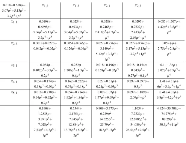
Here we present a run of our algorithm ??, where the input data are taken from Raghavan and Syed (2002). There are 5 states, the first two are controlled by player 1 and states 3 and 4 are for player 2; in the final state both players have no action choice. The immediate rewards and the probability transitions for every couple (state,action) for both players are shown in table 1.

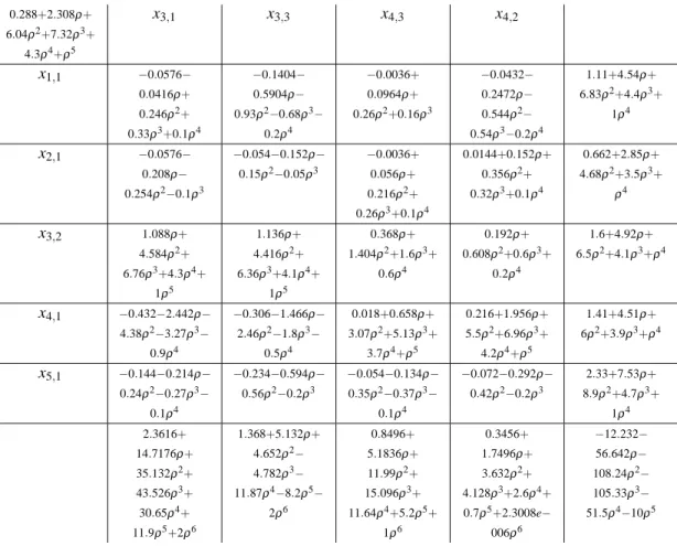
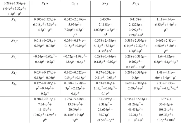
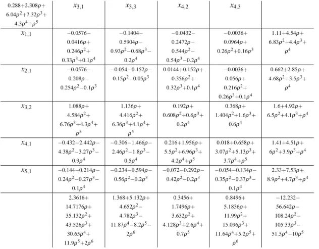
We choose the initial strategy (g(a2|s3) = 1, g(a3|s4) = 1) for player 2. We report the optimum

tableau obtained by player 1 at the end of step 2 of the first iteration of our algorithm (tab.4) and the tableau of player 2 after the first improvement at step 3 (tab.5). Analogously, the tableaux 6 and 7 are associated to the second and last iteration of our algorithm. It is known (see Hordijk et al. 1985) that all the elements of simplex tableaux have a common denominator, stored in the top left-hand box. The last column of each tableau contains the numerator of the value of the basic variables, which are listed in the first column. The last row indicates the numerator of the reduced costs.

The optimum long term average strategy for player 1 is f∗(a1|s1) = 1, f∗(a2|s2) = 1, and for

By computing the first positive root of the reduced costs of the two last optimal tableaux we find that the strategies(f∗_{, g}∗_{) are alsoβ-discount optimal for all the discount factorβ∈ [β}∗_{; 1), where} β∗∼_{= 0.74458.}

Note that the optimal strategies differ from the ones of Raghavan and Syed (2002), in which the discount factor is set to 0.999. We suspect that this is due to some clerical errors.

8

A lower complexity algorithm

LetΓbe a zero-sum two-player stochastic game with perfect information. Consider the following

algorithm: This is essentially a best reponse algorithm, in which at each step each player alternatively

Step 1 Choose a stationary pure strategy g0for player 2. Set k := 0.

Step 2 Find the Blackwell optimal strategy fkfor player 1 in the MDPΓ1(gk).

Step 3 If gkis Blackwell optimal inΓ2(fk), then set (f∗, g∗) := (fk, gk) and stop. Otherwise, find the Blackwell optimal strategy gk+1for player 2 in the MDPΓ2(fk), set k := k + 1 and go to step 2.

looks for his own Blackwell optimal strategy.

Obviously, if the above algorithm stops,(f∗, g∗) forms a couple of uniform discount and long term

average optimal strategies, since they are both Blackwell optimal in the respective MDPs,Γ1(g∗)

andΓ2(f∗).

The proof that the algorithm ?? never cycles is still an open problem. It is quite natural to try to prove thatΦ_ρ(fk+1, gk+1) ≤lΦρ(fk, gk), but it is not difficult to find a counterexample.

Raghavan and Syed (2002) conjecture as follows:

Conjecture 8.1. LetΓ be a two-player zero-sum stochastic game with perfect information and

α= (f, g) a couple of pure stationary strategies for the 2 players. For every discount factorβ∈ [0; 1),

there are no sequencesα0,α1, . . . ,αksuch thatΦ_β(αk) =Φ_β(α0), whereαiis an adjacent

improve-ment with respect toαi−1in theβ-discounted stochastic gameΓfor only one player for any i> 0.

If Conjecture 8.1 were valid, then we could conclude that the algorithm ?? terminates in finite time.

8.1

Complexity

In our first algorithm ??, player 1 faces at each step an MDP optimization problem in the field of rational functions with real coefficients, which is solvable in polynomial time. Player 2, instead, is

involved in a lexicographic search throughout the algorithm unfolding, whose complexity is at worst exponential in time.

Player 2 lexicographically expands his search of his optimum strategy, and at the k-th iteration the two players find the solution of a subgameΓkwhich monotonically tends to the entire stochastic gameΓ.

Analogously to what Raghavan and Syed (2002) remark, we can assert that the efficiency of our algorithm ?? is mostly due to the fact that most of the actions dominate totally other actions. In other words, it occurs very often that the optimum action a∗∈ A(s), s ∈ S, found in an iteration k such that

A(s) ⊂Γk, is optimum also inΓ, and consequently remains the same in all the remaining iterations. This exponentially reduces the policy space in which the algorithm needs to search.

Remark 4. As discussed in section 6, in the algorithm ?? players’ roles are interchangeble. Since

most of the actions dominate totally other actions, we suggest to assign the step 2 of the algorithm to the player whose total number of available actions is greater.

Differently from Raghavan and Syed (2002), the search for player 1 does not need to be lexico-graphic, and player 1 is left totally free to optimize the MDP that he faces at each iteration of the algorithm in the most efficient way.

Let us compare in terms of number of pivoting the following three algorithms:

M₁: Algorithm ??, in which in step 2 player 1 pivots with respect to the variable with the minimum reduced cost until he finds his own Blackwell optimal strategy.

M₂: Algorithm ??, in which in step 2 player 1 pursues a lexicographic search, pivoting iteratively with respect to the first non-basic variable with a negative (in the field F(R)) reduced cost.

This method is analogous to the one shown by Raghavan and Syed (2002), but in the field

F(R).

M3: Algorithm ??.

The results are shown in tables 2 and 3. The simulations were carried out on 10000 randomly generated stochastic games with 4 states, 2 for player 1 and 2 for player 2. In each state 5 actions are available for the controlling player.

Table 2: Average number of pivotings for the 3 methods.

n. pivoting

M1 40.59

M2 41.87

M3 24.93

It is evident that the algorithm M3is much faster than the other two, but unfortunately its

con-vergence is not proven yet. However, in our numerical experiment with 10000 randomly generated stochastic games, it never cycles. The difference between M1and M2is due to the more efficient

Table 3: Mi> Mjwhen, fixing the game, the number of pivotings in Miis strictly smaller

than the number of pivoting in Mj.

> (%) M1 M2 M3

M1 - 52.85 18.57

M2 42.18 - 15.26

M3 80.05 82.75

-Table 4: Optimum tableau for player 1 at the first iteration.

0.018+0.658ρ+ 3.07ρ2_+5.13ρ3₊ 3.7ρ4_+ρ5 x1,2 x1,3 x2,1 x2,3 x1,1 0.0198+ 0.6698ρ+ 3.06ρ2_+5.11ρ3₊ 3.7ρ4_+ρ5 0.0234+ 0.6934ρ+ 3.04ρ2_+5.07ρ3₊ 3.7ρ4_+ρ5 0.0288+ 0.7468ρ+ 2.418ρ2_+2.7ρ3₊ ρ4 0.0297+ 0.7527ρ+ 2.413ρ2₊ 2.69ρ3_+ρ4 0.087+1.707ρ+ 4.42ρ2_+3.8ρ3₊ ρ4 x2,2 0.0018+0.022ρ+ 0.042ρ2_+0.02ρ3 0.0054+0.066ρ+ 0.126ρ2_+0.06ρ3 0.027+0.756ρ+ 3.149ρ2₊ 5.12ρ3_+3.7ρ4₊ 1ρ5 0.0279+0.767ρ+ 3.17ρ2_+5.13ρ3₊ 3.7ρ4_+1ρ5 0.059+ρ+ 2.75ρ2_+2.8ρ3₊ ρ4 x3,1 −0.084ρ− 0.402ρ2_−0.5ρ3₋ 0.2ρ4 −0.252ρ− 1.206ρ2_−1.5ρ3₋ 0.6ρ4 0.018+0.196ρ+ 0.158ρ2_−0.02ρ3 0.018+0.154ρ− 0.043ρ2₋ 0.27ρ3_−0.1ρ4 0.1+1.36ρ+ 3.07ρ2_+2.9ρ3₊ ρ4 x4,1 0.054+0.174ρ+ 0.18ρ2_+0.06ρ3 0.162+0.522ρ+ 0.54ρ2_+0.18ρ3 0.27+0.51ρ+ 0.21ρ2_−0.03ρ3 0.297+0.597ρ+ 0.3ρ2 1.41+4.51ρ+ 6ρ2+3.9ρ3_+1ρ4 x5,1 0.018+0.238ρ+ 0.64ρ2_+0.62ρ3₊ 0.2ρ4 0.054+0.714ρ+ 1.92ρ2_+1.86ρ3₊ 0.6ρ4 0.09+1.07ρ+ 1.77ρ2_+0.69ρ3₋ 0.1ρ4 0.099+1.189ρ+ 2.09ρ2_+ρ3 0.41+4.01ρ+ 6.8ρ2_+4.2ρ3_+ρ4 0.1908+ 1.2838ρ+ 3.891ρ2₊ 7.028ρ3₊ 7.53ρ4_+4.3ρ5₊ 1ρ6 0.5544+ 3.1754ρ+ 7.945ρ2₊ 12.884ρ3₊ 13.76ρ4_+8.2ρ5₊ 2ρ6 0.909+3.373ρ+ 0.229ρ2₋ 14.525ρ3₋ 25.79ρ4₋ 18.5ρ5_−5ρ6 1.1034+ 7.7329ρ+ 22.6785ρ2₊ 34.089ρ3₊ 26.54ρ4_+9.5ρ5₊ 1ρ6 4.924+30.709ρ+ 74.775ρ2₊ 88.29ρ3₊ 50.3ρ4_+11ρ5

References

[1] E. Altman, K. Avrachenkov and J.A. Filar, Asymptotic linear programming and policy improve-ment for singularly perturbed Markov decision processes, ZOR: Mathematical Methods of Oper-ations Research, Vol.49, No.1, pp.97-109 (1999).

Table 5: Optimum tableau for player 2 at the first iteration. 0.288+2.308ρ+ 6.04ρ2_+7.32ρ3₊ 4.3ρ4_+ρ5 x3,1 x3,3 x4,3 x4,2 x1,1 −0.0576− 0.0416ρ+ 0.246ρ2₊ 0.33ρ3_+0.1ρ4 −0.1404− 0.5904ρ− 0.93ρ2_−0.68ρ3₋ 0.2ρ4 −0.0036+ 0.0964ρ+ 0.26ρ2_+0.16ρ3 −0.0432− 0.2472ρ− 0.544ρ2₋ 0.54ρ3_−0.2ρ4 1.11+4.54ρ+ 6.83ρ2_+4.4ρ3₊ 1ρ4 x2,1 −0.0576− 0.208ρ− 0.254ρ2_−0.1ρ3 −0.054−0.152ρ− 0.15ρ2_−0.05ρ3 −0.0036+ 0.056ρ+ 0.216ρ2₊ 0.26ρ3_+0.1ρ4 0.0144+0.152ρ+ 0.356ρ2₊ 0.32ρ3_+0.1ρ4 0.662+2.85ρ+ 4.68ρ2_+3.5ρ3₊ ρ4 x3,2 1.088ρ+ 4.584ρ2₊ 6.76ρ3_+4.3ρ4₊ 1ρ5 1.136ρ+ 4.416ρ2₊ 6.36ρ3_+4.1ρ4₊ 1ρ5 0.368ρ+ 1.404ρ2_+1.6ρ3₊ 0.6ρ4 0.192ρ+ 0.608ρ2_+0.6ρ3₊ 0.2ρ4 1.6+4.92ρ+ 6.5ρ2_+4.1ρ3_+ρ4 x4,1 −0.432−2.442ρ− 4.38ρ2_−3.27ρ3₋ 0.9ρ4 −0.306−1.466ρ− 2.46ρ2_−1.8ρ3₋ 0.5ρ4 0.018+0.658ρ+ 3.07ρ2_+5.13ρ3₊ 3.7ρ4_+ρ5 0.216+1.956ρ+ 5.5ρ2_+6.96ρ3₊ 4.2ρ4_+ρ5 1.41+4.51ρ+ 6ρ2+3.9ρ3_+ρ4 x5,1 −0.144−0.214ρ− 0.24ρ2_−0.27ρ3₋ 0.1ρ4 −0.234−0.594ρ− 0.56ρ2_−0.2ρ3 −0.054−0.134ρ− 0.35ρ2_−0.37ρ3₋ 0.1ρ4 −0.072−0.292ρ− 0.42ρ2_−0.2ρ3 2.33+7.53ρ+ 8.9ρ2_+4.7ρ3₊ 1ρ4 2.3616+ 14.7176ρ+ 35.132ρ2₊ 43.526ρ3₊ 30.65ρ4₊ 11.9ρ5_+2ρ6 1.368+5.132ρ+ 4.652ρ2₋ 4.782ρ3₋ 11.87ρ4_−8.2ρ5₋ 2ρ6 0.8496+ 5.1836ρ+ 11.99ρ2₊ 15.096ρ3₊ 11.64ρ4_+5.2ρ5₊ 1ρ6 0.3456+ 1.7496ρ+ 3.632ρ2₊ 4.128ρ3_+2.6ρ4₊ 0.7ρ5_+2.3008e− 006ρ6 −12.232− 56.642ρ− 108.24ρ2₋ 105.33ρ3₋ 51.5ρ4_−10ρ5

Table 6: Optimum tableau for player 1 at the second iteration. 0.288+2.308ρ+ 6.04ρ2_+7.32ρ3₊ 4.3ρ4_+ρ5 x1,2 x1,3 x2,1 x2,3 x1,1 0.306+2.324ρ+ 6.018ρ2_+7.3ρ3₊ 4.3ρ4_+ρ5 0.342+2.356ρ+ 5.974ρ2₊ 7.26ρ3_+4.3ρ4₊ ρ5 0.4068+ 2.1148ρ+ 4.008ρ2_+3.3ρ3₊ ρ4 0.4158+ 2.1228ρ+ 3.997ρ2₊ 3.29ρ3_+ρ4 1.11+4.54ρ+ 6.83ρ2_+4.4ρ3₊ ρ4 x2,2 0.018+0.058ρ+ 0.06ρ2_+0.02ρ3 0.054+0.174ρ+ 0.18ρ2_+0.06ρ3 0.378+2.478ρ+ 6.11ρ2_+7.31ρ3₊ 4.3ρ4_+ρ5 0.387+2.507ρ+ 6.14ρ2_+7.32ρ3₊ 4.3ρ4_+ρ5 0.662+2.85ρ+ 4.68ρ2_+3.5ρ3₊ ρ4 x3,1 −0.24ρ−0.66ρ2₋ 0.62ρ3_−0.2ρ4 −0.72ρ−1.98ρ2₋ 1.86ρ3_−0.6ρ4 0.288+0.436ρ+ 0.128ρ2_−0.02ρ3 0.288+0.316ρ− 0.202ρ2₋ 0.33ρ3_−0.1ρ4 1.6+4.92ρ+ 6.5ρ2_+4.1ρ3_+ρ4 x4,1 0.054+0.174ρ+ 0.18ρ2_+0.06ρ3 0.162+0.522ρ+ 0.54ρ2_+0.18ρ3 0.27+0.51ρ+ 0.21ρ2_−0.03ρ3 0.297+0.597ρ+ 0.3ρ2 1.41+4.51ρ+ 6ρ2+3.9ρ3_+ρ4 x5,1 0.126+0.586ρ+ ρ2_+0.74ρ3₊ 0.2ρ4 0.378+1.758ρ+ 3ρ2_+2.22ρ3₊ 0.6ρ4 0.63+2.09ρ+ 2.19ρ2_+0.63ρ3₋ 0.1ρ4 0.693+2.383ρ+ 2.69ρ2_+ρ3 2.33+7.53ρ+ 8.9ρ2_+4.7ρ3_+ρ4 0.504+2.818ρ+ 7.344ρ2₊ 11.15ρ3₊ 10.02ρ4_+4.9ρ5₊ ρ6 1.224+5.858ρ+ 13.684ρ2₊ 20.09ρ3₊ 18.44ρ4_+9.4ρ5₊ 2ρ6 1.8+2.896ρ− 8.318ρ2₋ 29.624ρ3₋ 36.71ρ4₋ 21.5ρ5_−5ρ6 3.636+18.583ρ+ 41.268ρ2₊ 49.431ρ3₊ 32.21ρ4₊ 10.1ρ5_+ρ6 12.232+ 56.642ρ+ 108.24ρ2₊ 105.33ρ3₊ 51.5ρ4_+10ρ5

Table 7: Optimum tableau for player 2 at the second iteration. 0.288+2.308ρ+ 6.04ρ2_+7.32ρ3₊ 4.3ρ4_+ρ5 x3,1 x3,3 x4,2 x4,3 x1,1 −0.0576− 0.0416ρ+ 0.246ρ2₊ 0.33ρ3_+0.1ρ4 −0.1404− 0.5904ρ− 0.93ρ2_−0.68ρ3₋ 0.2ρ4 −0.0432− 0.2472ρ− 0.544ρ2₋ 0.54ρ3_−0.2ρ4 −0.0036+ 0.0964ρ+ 0.26ρ2_+0.16ρ3 1.11+4.54ρ+ 6.83ρ2_+4.4ρ3₊ ρ4 x2,1 −0.0576− 0.208ρ− 0.254ρ2_−0.1ρ3 −0.054−0.152ρ− 0.15ρ2_−0.05ρ3 0.0144+0.152ρ+ 0.356ρ2₊ 0.32ρ3_+0.1ρ4 −0.0036+ 0.056ρ+ 0.216ρ2₊ 0.26ρ3_+0.1ρ4 0.662+2.85ρ+ 4.68ρ2_+3.5ρ3₊ ρ4 x3,2 1.088ρ+ 4.584ρ2₊ 6.76ρ3_+4.3ρ4₊ ρ5 1.136ρ+ 4.416ρ2₊ 6.36ρ3_+4.1ρ4₊ ρ5 0.192ρ+ 0.608ρ2_+0.6ρ3₊ 0.2ρ4 0.368ρ+ 1.404ρ2_+1.6ρ3₊ 0.6ρ4 1.6+4.92ρ+ 6.5ρ2_+4.1ρ3_+ρ4 x4,1 −0.432−2.442ρ− 4.38ρ2_−3.27ρ3₋ 0.9ρ4 −0.306−1.466ρ− 2.46ρ2_−1.8ρ3₋ 0.5ρ4 0.216+1.956ρ+ 5.5ρ2_+6.96ρ3₊ 4.2ρ4_+ρ5 0.018+0.658ρ+ 3.07ρ2_+5.13ρ3₊ 3.7ρ4_+ρ5 1.41+4.51ρ+ 6ρ2+3.9ρ3_+ρ4 x5,1 −0.144−0.214ρ− 0.24ρ2_−0.27ρ3₋ 0.1ρ4 −0.234−0.594ρ− 0.56ρ2_−0.2ρ3 −0.072−0.292ρ− 0.42ρ2_−0.2ρ3 −0.054−0.134ρ− 0.35ρ2_−0.37ρ3₋ 0.1ρ4 2.33+7.53ρ+ 8.9ρ2_+4.7ρ3_+ρ4 2.3616+ 14.7176ρ+ 35.132ρ2₊ 43.526ρ3₊ 30.65ρ4₊ 11.9ρ5_+2ρ6 1.368+5.132ρ+ 4.652ρ2₋ 4.782ρ3₋ 11.87ρ4_−8.2ρ5₋ 2ρ6 0.3456+ 1.7496ρ+ 3.632ρ2₊ 4.128ρ3_+2.6ρ4₊ 0.7ρ5 0.8496+ 5.1836ρ+ 11.99ρ2₊ 15.096ρ3₊ 11.64ρ4_+5.2ρ5₊ ρ6 −12.232− 56.642ρ− 108.24ρ2₋ 105.33ρ3₋ 51.5ρ4_−10ρ5

[2] E. Altman, E. A. Feinberg, A. Shwartz, Weighted discounted stochastic games with perfect information, Annals of the International Society of Dynamic Games, Vol. 5, pp. 303-324 (2000). [3] T. Bewley, E. Kohlberg, The asymptotic theory of stochastic games, Mathematics of Operations

Research, Vol. 1, No. 3, pp. 197-208 (1976).

[4] K. Chatterjee, R. Majumdar, T.A. Henzinger, Stochastic limit-average games are in EXPTIME, International Journal of Game Theory, Vol. 37, No. 2, pp. 219-234 (2008).

[5] B.C. Eaves, U.G. Rothblum, Formulation of linear problems and solution by a universal ma-chine, Mathematical Programming, Vol. 65, No. 1-3, pp. 263-309 (1994).

[6] J. Filar, K. Vrieze, Competitive Markov Decision Processes, Springer (1996).

[7] J.A. Filar, E. Altman and K. Avrachenkov, An asymptotic simplex method for singularly per-turbed linear programs, Operations Research Letters, Vol. 30, No. 5, pp. 295-307 (2002). [8] D. Gillette, Stochastic games with zero stop probabilities, Contributions to the theory of games,

Princeton University Press, Vol. 3, pp. 179-187 (1957).

[9] A. Hordijk, R. Dekker, L.C.M. Kallenberg, Sensitivity Analysis in Discounted Markov Decision Processes, OR Spektrum, Vol. 7, No. 3, pp. 143-151 (1985).

[10] D.G. Luenberger, Y. Ye, Linear and nonlinear programming (Third ed.), Springer (2008). [11] J.F. Mertens, A. Neyman, Stochastic games, International Journal of Game Theory, Vol. 10,

pp. 53-66 (1981).

[12] T. Parthasarathy, T.E.S. Raghavan, An orderfield property for stochastic games when one player controls transition probabilities, Journal of Optimization Theory and Applications, Vol. 33, No. 3, pp. 375-392 (1981).

[13] M. L. Puterman, Markov Decision Processes: Discrete Stochastic Dynamic Programming, Wi-ley (1994).

[14] T.E.S. Raghavan, Z. Syed, A policy-improvement type algorithm for solving zero-sum two-person stochastic games of perfect information, Mathematical Programming, Vol. 95, No. 3, pp. 513-532 (2003).

[15] L.S. Shapley, Stochastic games, Proceedings of the National Academy of Sciences USA, Vol. 39, pp. 1095-1100 (1953).

[16] E. Solan, N. Vieille, Computing uniformly optimal strategies in two-player stochastic games, Economic Theory, Vol. 42, No. 1, pp. 237-253 (2010).

[17] F. Thuijsman, T.E.S. Raghavan, Perfect information stochastic games and related classes, In-ternational Journal of Game Theory, Vol. 26, pp. 403-408 (1997).

Unité de recherche INRIA Futurs : Parc Club Orsay Université - ZAC des Vignes 4, rue Jacques Monod - 91893 ORSAY Cedex (France)

Unité de recherche INRIA Lorraine : LORIA, Technopôle de Nancy-Brabois - Campus scientifique 615, rue du Jardin Botanique - BP 101 - 54602 Villers-lès-Nancy Cedex (France)

Unité de recherche INRIA Rennes : IRISA, Campus universitaire de Beaulieu - 35042 Rennes Cedex (France) Unité de recherche INRIA Rhône-Alpes : 655, avenue de l’Europe - 38334 Montbonnot Saint-Ismier (France) Unité de recherche INRIA Rocquencourt : Domaine de Voluceau - Rocquencourt - BP 105 - 78153 Le Chesnay Cedex (France)