Building efficient algorithms by learning to compress

Building Efficient Algorithms by

Learning to Compress

by

Davis W. Blalock

B.S., University of Virginia (2014)

S.M., Massachusetts Institute of Technology (2016)

Submitted to the Department of Electrical Engineering and Computer

Science

in partial fulfillment of the requirements for the degree of

Doctor of Philosophy in Electrical Engineering and

Computer Science

at the

MASSACHUSETTS INSTITUTE OF TECHNOLOGY

September 2020

© Davis W. Blalock, MMXX. All rights reserved.

The author hereby grants to MIT permission to reproduce and to

distribute publicly paper and electronic copies of this thesis document

in whole or in part in any medium now known or hereafter created.

Author . . . .

Department of Electrical Engineering and Computer Science

August 28, 2020

Certified by . . . .

John V. Guttag

Thesis Supervisor

Accepted by . . . .

Leslie A. Kolodziejski

Professor of Electrical Engineering and Computer Science

Chair, Department Committee on Graduate Students

Building Efficient Algorithms by

Learning to Compress

by

Davis W. Blalock

Submitted to the Department of Electrical Engineering and Computer Science on August 28, 2020, in partial fulfillment of the

requirements for the degree of

Doctor of Philosophy in Electrical Engineering and Computer Science

Abstract

The amount of data in the world is doubling every two years. Such abundant data offers immense opportunities, but also imposes immense computation, storage, and energy costs. This thesis introduces efficient algorithms for reducing these costs for bottlenecks in real world data analysis and machine learning pipelines.

Concretely, we introduce algorithms for:

• Lossless compression of time series. This algorithm compresses better than any existing method, despite requiring only the resources available on a low-power edge device.

• Approximate matrix-vector multiplies. This algorithm accelerates approximate sim-ilarity scans by an order of magnitude relative to existing methods.

• Approximate matrix-matrix multiplies. This algorithm often outperforms existing approximation methods by more than 10× and non-approximate computation by more than 100×.

We provide extensive empirical analyses of all three algorithms using real-world datasets and realistic workloads. We also prove bounds on the errors introduced by the two approximation algorithms.

The theme unifying all of these contributions is learned compression. While com-pression is typically thought of only as a means to reduce data size, we show that specially designed compression schemes can also dramatically increase computation speed and reduce memory requirements.

Thesis Supervisor: John V. Guttag

Acknowledgments

This PhD would not have been possible without the support and efforts of many people.

At the top of this list is my advisor, John Guttag. It’s difficult to identify all the positive aspects of having John as an advisor, so I will stick to only a few key points. First, John is extremely supportive and kind—he genuinely wants what’s best for his graduate students and is generous and understanding far beyond the call of duty. In addition, one could not ask for a more knowledgeable mentor; John has deep expertise in many areas of computer science, and I doubt I could have tackled the problems I did without his willingness and ability to straddle many subfields at once. This knowledgeability also extends to the practice of research itself; John can often transform writing, presentations, and problem framings from lackluster to exceptional in the span of a single round of feedback.

I am also indebted to my collaborators and labmates. I would particularly like to thank Divya Shanmugam and Jose Javier Gonzalez Ortiz for managing to put up with me over the course of multiple research projects. I would also like to thank Anima, Yun, Guha, Joel, Jen, Amy, Maggie, Adrian, Tristan, Marzyeh, Tiam, Harini, Katie, Marianne, Emily, Addie, Wayne, Sra, Matt, Dina, Maryann, Roshni, and Aniruddh for their friendship, feedback, and ideas over the years.

Along similar lines, I would like to thank Sam Madden and Tamara Broderick for serving on my thesis committee and being great collaborators in research (and other) endeavors in the past few years. Sam and Tamara not only possess deep expertise in their fields, but are also enjoyable and interesting to work with.

I would be remiss not to include some mentors from before MIT. Foremost, I’d like to thank John Lach and Ben Boudaoud for taking a chance on me when I was an undergrad who didn’t know anything. I’d also like to thank Jeff, Kevin, Jermaine, Jim, Jake, Drake, and the rest of the PocketSonics team for mentoring me throughout many years of internships.

influence on me getting where I am today. But seriously, I could never thank them enough or adequately describe their positive impact on my life in a paragraph, so I will just note that I’m profoundly grateful for all the sacrifices they’ve made for me and for the good fortune of getting to be part of this family.

Contents

1 Introduction 15

2 Compressing Integer Time Series 19

2.1 Introduction . . . 19

2.2 Definitions and Background . . . 22

2.2.1 Definitions . . . 22

2.2.2 Hardware Constraints . . . 22

2.2.3 Data Characteristics . . . 23

2.3 Related Work . . . 24

2.3.1 Compression of Time Series . . . 24

2.3.2 Compression of Integers . . . 25 2.3.3 General-Purpose Compression . . . 26 2.3.4 Predictive Filtering . . . 26 2.4 Method . . . 27 2.4.1 Overview . . . 27 2.4.2 Forecasting . . . 29 2.4.3 Bit Packing . . . 33 2.4.4 Entropy Coding . . . 36 2.4.5 Vectorization . . . 36 2.5 Experimental Results . . . 37 2.5.1 Datasets . . . 37 2.5.2 Comparison Algorithms . . . 38 2.5.3 Compression Ratio . . . 39

2.5.4 Decompression Speed . . . 42

2.5.5 Compression Speed . . . 43

2.5.6 FIRE Speed . . . 45

2.5.7 When to Use Sprintz . . . 46

2.5.8 Generalizing to Floats . . . 48

2.6 Summary . . . 50

3 Fast Approximate Scalar Reductions 51 3.1 Introduction . . . 51

3.1.1 Problem Statement . . . 53

3.1.2 Assumptions . . . 54

3.2 Related Work . . . 55

3.3 Method . . . 57

3.3.1 Background: Product Quantization . . . 57

3.3.2 _Bolt . . . 61 3.3.3 Theoretical Guarantees . . . 64 3.4 Experimental Results . . . 65 3.4.1 Datasets . . . 66 3.4.2 Comparison Algorithms . . . 67 3.4.3 Encoding Speed . . . 68 3.4.4 Query Speed . . . 68

3.4.5 Nearest Neighbor Accuracy . . . 72

3.4.6 Accuracy in Preserving Distances and Dot Products . . . 74

3.5 Summary . . . 75

4 Fast Approximate Matrix Multiplication 77 4.1 Introduction . . . 77

4.1.1 Problem Formulation . . . 79

4.2 Related Work . . . 79

4.2.1 Linear Approximation . . . 80

4.3 Background - Product Quantization . . . 81

4.4 Our Method . . . 83

4.4.1 Hash Function Family, 𝑔(·) . . . 83

4.4.2 Learning the Hash Function Parameters . . . 84

4.4.3 Optimizing the Prototypes . . . 86

4.4.4 Fast 8-Bit Aggregation, 𝑓 (·, ·) . . . . 87

4.4.5 Complexity . . . 88

4.4.6 Theoretical Guarantees . . . 89

4.5 Experiments . . . 90

4.5.1 Methods Tested . . . 91

4.5.2 _{How Fast is Maddness? . . . .} 92

4.5.3 Softmax Classifier . . . 93

4.5.4 Kernel-Based Classification . . . 94

4.5.5 Image Filtering . . . 96

4.6 Summary . . . 97

5 Summary and Conclusion 99 A Additional Theoretical Analysis of Bolt 103 A.1 Quantization Error . . . 103

A.1.1 Definitions . . . 103

A.1.2 Guarantees . . . 105

A.2 Dot Product Error . . . 108

A.2.1 Definitions and Preliminaries . . . 108

A.2.2 Guarantees . . . 112

A.2.3 Euclidean Distance Error . . . 114

B Additional Theoretical Analysis of Maddness 119 B.1 Proof of Generalization Guarantee . . . 119

C Additional Method and Experiment Details for Maddness 129

C.1 Quantizing Lookup Tables . . . 129

C.2 Quantization and MaddnessHash . . . 130

C.3 Subroutines for Training MaddnessHash . . . 131

C.4 Additional Experimental Details . . . 131

C.4.1 Exact Matrix Multiplication . . . 132

C.4.2 Additional Baselines . . . 132

C.4.3 UCR Time Series Archive . . . 133

C.4.4 Caltech101 . . . 134

List of Figures

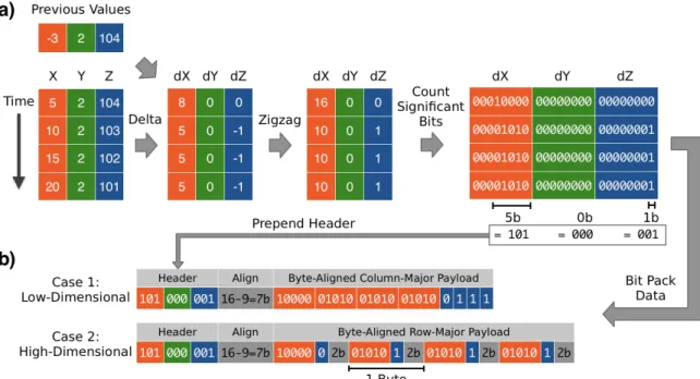
2-1 _{Overview of Sprintz using a delta coding predictor. a) Delta} cod-ing of each column, followed by zigzag encodcod-ing of resultcod-ing errors. The maximum number of significant bits is computed for each col-umn. b) These numbers of bits are stored in a header, and the original data is stored as a byte-aligned payload, with leading zeros removed. When there are few columns, each column’s data is stored contigu-ously. When there are many columns, each row is stored contiguously, possibly with padding to ensure alignment on a byte boundary. . . . 34 2-2 Boxplots of compression performance of different algorithms on the

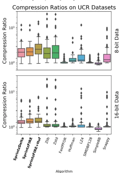
UCR Time Series Archive. Each boxplot captures the distribution of one algorithm across all 85 datasets. . . 40 2-3 Compression performance of different algorithms on the UCR Time

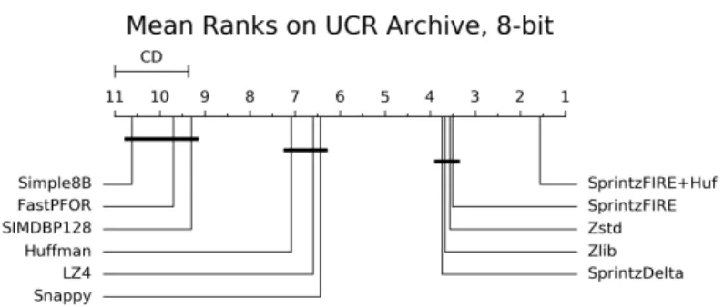
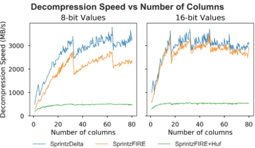
Series Archive. The x-axis is the mean rank of each method, where rank 1 on a given dataset has the highest ratio. Methods joined with a horizontal black line are not statistically significantly different. . . . 42 2-4 _{Sprintz becomes faster as the number of columns increases and as}

the width of each sample approaches multiples of 32B (on a machine with 32B vector registers). . . 44 2-5 _{Sprintz compresses at hundreds of MB/s even in the slowest case: its}

highest-ratio setting with incompressible 8-bit data. On lower settings with 16-bit data, it can exceed 1GB/s. . . 44

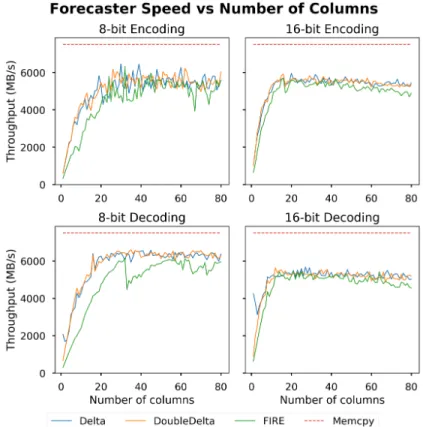
2-6 _{Fire is nearly as fast as delta and double delta coding. For a moderate} number of columns, it runs at 5-6GB/s on a machine with 7.5GB/s memcpy speed. . . 45 2-7 _{Sprintz achieves excellent compression ratios and speed on relatively}

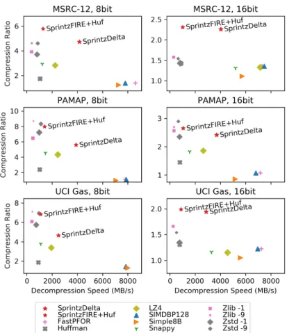
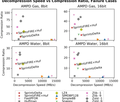
slow-changing time series with many variables. . . 47 2-8 _{Sprintz is less effective than other methods when the time series has}

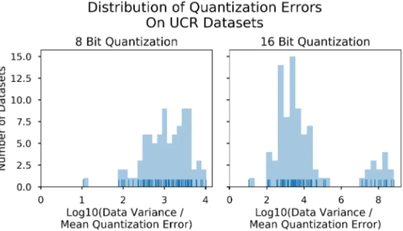
large, abrupt changes and few variables. . . 48 2-9 Quantizing floating point time series to integers introduces error that

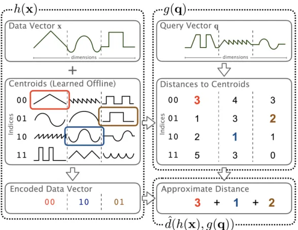
is orders of magnitude smaller than the variance of the data. Even with eight bits, quantization introduces less than 1% error on 82 of 85 datasets. . . 49 3-1 Product Quantization. The ℎ(·) function returns the index of the most

similar centroid to the data vector 𝑥 in each subspace. The 𝑔(·) func-tion computes a lookup table of distances between the query vector 𝑞 and each centroid in each subspace. The aggregation function ^𝑑(·, ·)

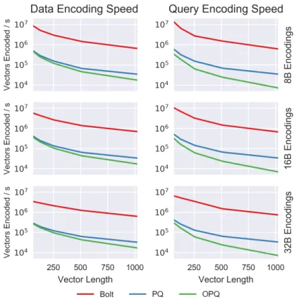
sums the table entries corresponding to each index. . . 58 3-2 _{Bolt encodes both data and query vectors significantly faster than}

similar algorithms. . . 69 3-3 _{Bolt can compute the distances or similarities between a query and}

the vectors of a compressed database up to 10× faster than other MCQ algorithms. It is also faster than binary embedding methods, which use the hardware popcount instruction, and matrix-vector multiplies using batches of 1, 256, or 1024 vectors. . . 70 3-4 _{Using a naive nested loop implementation, Bolt can compute}

approx-imate matrix products faster than optimized matrix multiply routines. Except for small matrices, Bolt is faster even when it must encode the matrices from scratch as a first step. . . 71 3-5 _{Compared to other MCQ algorithms, Bolt is slightly less accurate in}

3-6 _{Bolt dot products are highly correlated with true dot products, though} slightly less so than those from other MCQ algorithms. . . 75 4-1 _{Maddness encodes the 𝐴 matrix orders of magnitude more quickly}

than existing vector quantization methods. . . 93 4-2 _{Given the preprocessed matrices, Maddness computes the}

approxi-mate output twice as fast as the fastest existing method. . . 93 4-3 _{Maddness achieves a far better speed-accuracy tradeoff than any}

ex-isting method when approximating two softmax classifiers. . . 94 4-4 Fraction of UCR datasets for which each method preserves a given

fraction of the original accuracy versus the method’s degree of speedup. Maddness enables much greater speedups for a given level of accuracy degradation. . . 95 4-5 _{Despite there being only two columns in the matrix 𝐵, Maddness still}

achieves a significant speedup with reasonable accuracy. Methods that are Pareto dominated by exact matrix multiplication on both tasks are not shown; this includes all methods but Maddness and SparsePCA. 96 C-1 Maddness achieves a far better speed versus squared error tradeoff

than any existing method when approximating two softmax classifiers. These results parallel the speed versus classification accuracy results, except that the addition of our ridge regression is much more beneficial on CIFAR-100. . . 135 C-2 Maddness also achieves a far better speed versus accuracy tradeoff

when speed is measured as number of operations instead of wall time. Fewer operations with a high accuracy (up and to the left) is better. . 136

Chapter 1

Introduction

As datasets grow larger, so too do the costs of using them. These costs come in the form of computation, storage, memory, network, and energy usage. This thesis introduces algorithms to reduce these costs for various common elements of real-world data collection and analysis pipelines.

The central theme of our work is using machine learning to construct and manipu-late efficient, low-level representations of data. We show that by learning to compress data into specific, algorithm-friendly formats, we can obtain dramatic speed and space savings—often 10× to 100×—compared to either the original data or vector-valued embeddings. This is not merely a matter of quantizing floating point scalars, projecting data into lower-dimensional spaces, or otherwise employing well-known techniques; it is instead a matter of examining the “full stack,” from application requirements to processor instruction sets, in order to jointly formalize problems, de-fine efficient algorithms, and design compute-friendly data representations. Where applicable, we also prove theoretical guarantees about the resulting methods.

To make these claims more concrete, it is helpful to introduce the three problems discussed in this thesis:

Compression of time series data (Chapter 2). Time series constitute a large and growing fraction of the world’s data, but there has been little work on how best to compress them. Such compression is especially important at the point of

collection; low-power devices such as wearable health trackers must expend a great deal of energy to transmit data, so reductions in data size yield vital reductions in power consumption. We introduce a lossless compression algorithm for time series that achieves state-of-the-art compression ratios and speed, despite using only the limited resources available on low-power hardware. A key element of this method is an algorithm for simultaneous online prediction of and training on samples that operates at over 5GB/s in a single CPU thread. This extreme speed makes it practical to replace fixed compression heuristics with a learned model, yielding significant space savings.

One application of this method is in gathering data from fitness wearables for gesture and activity recognition. This task is difficult and has attracted enormous attention both in industry [7, 119, 8, 6] and academia [88, 134, 135, 136, 89, 151, 30, 66, 21]. In order to construct accurate recognition models, it is desirable to collect as much accelerometer, gyroscope, and other data from each device as possible. However, transmitting this data from a wearable device to a phone or the cloud consumes precious battery life. This has led to interest in on-device compression [21]. We demonstrate using numerous datasets acquired from both wearable devices and a wide range of other sensors that our compression algorithm significantly outperforms existing alternatives. Moreover, it does so despite using 100× less memory than many competing methods.

Acceleration of Similarity Scans (Chapter 3). Similarity search is one of the core operations behind modern web and mobile applications. Such searches decom-pose into a coarse retrieval step and a linear scan step. We describe an algorithm to dramatically accelerate the linear scan step. It is conceptually similar to existing linear scan algorithms, but achieves large speedups by taking into account character-istics of modern hardware. The core of the method is a learning-based algorithm for compressing the database being searched, along with a compression format that can be scanned without decompressing the data.

image retrieval at Google [79, 163] and Facebook [4]. We demonstrate our method’s superiority on various benchmark datasets for both similarity search in general and image retrieval in particular.

Fast Approximate Matrix Products (Chapter 4). Matrix multiplication is one of the most fundamental operations in machine learning and data analysis. It is also the computational bottleneck in many workloads. We introduce an algorithm to quickly approximate matrix products that greatly outperforms existing methods for realistic matrix sizes. Our approach is a significant methodological departure from most work in this area in two ways: first, it exploits a training dataset to learn useful approximations; and second, it uses nonlinear transformations of the matrices, a counter-intuitive approach when approximating linear operations. Our method is well suited for accelerating neural network layers, which have linear operations as their computational bottleneck.

As stated previously, these methods are unified by a pattern of learning efficient representations and designing algorithms that exploit these representations.

In the first algorithm, we learn to represent time series as a sequence of low-bitwidth integers in a vectorizable data layout. The learning comes in the form of the online forecaster. Reducing space is the main focus, but, as we demonstrate, our compressed format can also be decompressed at extreme speed—often 2GB/s or more in a single CPU thread.

In the second algorithm, we learn to map vectors of floating point numbers to vectors of categorical values, each of which can be stored using only a few bits. This representation is both more compact than the original and much faster to operate on; for example, it allows us to approximate 256-element dot products in roughly two CPU cycles.

In the third algorithm, the form of the learned representations is the same as in the second, but the functions creating and using them are more efficient for matrix multiplication. First, we replace an exact clustering step with a learned

locality-sensitive hash function. Second, we replace an exact summation with a noisy estima-tor whose errors we analyze and correct for in closed form. And finally, we relax a set of constraints on parameters that other methods cannot relax without an immense performance penalty. These changes significantly increase quality for a given level of speed; among other results, we accelerate a softmax classifier on the CIFAR-10 dataset by a factor of 15× with only a .25% drop in accuracy, or over 100× with a 1.1% drop in accuracy, while also compressing the input representation by factors of 128× and 512× respectively. Our second algorithm, as well as all other existing methods, are more than an order of magnitude slower at these accuracies.

We discuss these three algorithms in more detail in Chapters 2-4, and conclude in Chapter 5 with additional observations and a discussion of the lessons that can be drawn from this work.

Chapter 2

Compressing Integer Time Series

2.1

Introduction

Thanks to the proliferation of smartphones, wearables, autonomous vehicles, and other connected devices, it is becoming common to collect large quantities of sensor-generated time series. Once this data is centralized in servers, many tools exist to analyze and create value from it [184, 50, 169, 160, 29, 178, 152, 162]. How-ever, centralizing the data can be challenging because of power constraints on the devices collecting it. In particular, transmitting data wirelessly is extremely power-intensive—on a representative set of chips [95, 96], transmitting data over Bluetooth Low Energy (BLE) costs tens of milliwatts, while computing at full power costs only tens of microwatts.

One strategy for reducing this power consumption is to extract information locally and only transmit summaries [172, 11, 35]. This can be effective in some cases, but requires both a predefined use case for which a summary is sufficient and an appropriate method of constructing this summary. Devising such a method can be a significant endeavor [172]. For common but difficult tasks such as gesture and activity recognition from wearables [7, 119, 8, 6, 88, 135, 136, 89, 151, 30, 66, 21], collecting large quantities of sensor data is desirable, and it is not clear how appropriate on-device summaries could be constructed; furthermore, even if some summarization method worked well for all present use cases, discarding the raw data would both

make further algorithmic advances difficult and reduce the competitive moat available to the device’s manufacturer.

A complementary and more general approach is to compress the data before trans-mitting it [11, 21, 93, 33, 170]. This allows arbitrary subsequent analysis and does not require elaborate summary construction algorithms. Unfortunately, existing com-pression methods either 1) are only applicable for specific types of data, such as time-stamps [148, 14, 118], audio [41, 154, 2, 138] or EEG [172, 124] recordings; or 2) use algorithms that are ill-suited to sensor-generated time series.

More specifically, existing methods (e.g., [122, 63, 133, 105, 43, 44, 55, 69, 116]) violate one or more of the following design requirements:

1. Small block size. On devices with only a few kilobytes of memory, it is not possible to buffer large amounts of data before compressing it. Moreover, even with more memory, buffering can add unacceptable latency; for example, a smartwatch transmitting nine axes of 8-bit motion data at 20Hz to a smartphone would need to wait 10000/(9 × 1 × 20) = 56 seconds to fill even a 10KB buffer. This precludes using this data for gesture recognition and would add unacceptable user interface latency for step counting, activity recognition, or most other purposes.

2. High decompression speed. While the device collecting the data may not need to decompress it, it is desirable to have an algorithm that could also function well in a central database. This eliminates the need to transcode the data at the server and simplifies the application. In a database, time series workloads are not only read-heavy [35, 14, 29], but often necessitate materializing data (or downsampled versions thereof) for visualization, clustering, computing correlations, or other operations [35]. At the same time, writing is often append-only [148, 35]. As a result, decompression speed is paramount, while compression speed need only be fast enough to keep up with the rate of data ingestion.

3. Lossless. Given that time series are almost always noisy and often oversampled, it might not seem necessary to compress them losslessly. However, noise and over-sampling 1) tend to vary across applications, and 2) are often best addressed in an application-specific way as a preprocessing step. Consequently, instead of assuming

that some level of downsampling or some particular smoothing will be appropriate for all data, it is better for the compression algorithm to preserve what it is given and leave preprocessing up to the application developer.

The primary contribution of this work is Sprintz, a compression algorithm for time series that offers state-of-the-art compression ratios and speed while also sat-isfying all of the above requirements. It requires <1KB of memory, can use blocks of data as small as eight samples, and can decompress at up to 3GB/s in a single thread. Sprintz’s effectiveness stems from exploiting 1) temporal correlations in each variable’s value and variance, and 2) the potential for parallelization across different variables, realized through the use of vector instructions. Sprintz operates directly only on integer time series. However, as we discuss in Section 2.5.8, straightforward preprocessing allows it to be applied to most floating point time series as well.

A key component of Sprintz’s operation is a novel, vectorized forecasting al-gorithm for integers. This alal-gorithm can simultaneously train online and generate predictions at close to the speed of memcpy, while significantly improving compres-sion ratios compared to delta coding.

A second contribution is an empirical comparison of a range of algorithms cur-rently used to compress time series, evaluated across a wide array of public datasets. We also make available code to easily reproduce these experiments, including the plots and statistical tests in the paper. To the best of our knowledge, this constitutes the largest public benchmark for time series compression.

The remainder of this paper is structured as follows. In Section 2.2, we introduce relevant definitions, background, and details regarding the problem we consider. In Section 4.2, we survey related work and what distinguishes Sprintz. In Sections 4.4 and 4.5, we describe Sprintz and evaluate it across a number of publicly-available datasets. We also discuss when Sprintz is advantageous relative to other approaches.

2.2

Definitions and Background

Before elaborating upon how our method works, we introduce necessary definitions and provide relevant information regarding the problem being solved.

2.2.1

Definitions

Definition 2.2.1. Sample. A sample is a vector 𝑥 ∈ R𝐷. 𝐷 is the sample’s di-mensionality. Each element of the sample is an integer represented using a number of bits 𝑤, the bitwidth. The bitwidth 𝑤 is shared by all elements.

Definition 2.2.2. Time Series. A time series 𝑋 of length 𝑇 is a sequence of 𝑇

samples, 𝑥1, . . . , 𝑥𝑇. All samples 𝑥𝑡 share the same bitwidth 𝑤 and dimensionality

𝐷. If 𝐷 = 1, 𝑋 is called univariate; otherwise it is multivariate.

Definition 2.2.3. Rows, Columns. When represented in memory, we assume that

each sample of a time series is one row and each dimension is one column. Because data arrives as samples and memory constraints may limit how many samples can be buffered, we assume that the data is stored in row-major order—i.e., such that each sample is stored contiguously.

2.2.2

Hardware Constraints

Many connected devices are powered by batteries or harvested energy [83]. This results in strict power budgets and, in order to satisfy them, omission of certain functionality. In particular, many devices lack hardware support for floating point operations, SIMD (vector) instructions, and integer division. Moreover, they often have no more than a few kilobytes of memory, clocks of tens of MHz at most, and 8-, 16-, or 32-bit processors instead of 64-bit [95, 96, 5].

In contrast, we assume that the hardware used to decompress the data does not share these limitations. It is likely a modern server with SIMD instructions, gigabytes of RAM, and a multi-GHz clock. However, because the amount of data it must

store and query can be large, compression ratio and decompression speed are still important.

2.2.3

Data Characteristics

From a compression perspective, time series have four attributes uncommon in other data.

1. Lack of exact repeats. In text or structured records, there are many sequences of bytes—often corresponding to words or phrases—that will exactly repeat many times. This makes dictionary-based methods a natural fit. In time series, however, the presence of noise makes exact repeats less common [30, 150].

2. Multiple variables. Real-world time series often consist of multiple variables that are collected and accessed together. For example, the Inertial Measurement Unit (IMU) in modern smartphones collects three-dimensional acceleration, gyroscope, and magnetometer data, for a total of nine variables sampled at each time step. These variables are also likely to be read together, since each on its own is insufficient to characterize the phone’s motion.

3. Low bitwidth. Any data collected by a sensor will be digitized into an integer by an Analog-to-Digital Converter (ADC). Nearly all ADCs have a precision of 32 bits or fewer [3], and typically 16 or fewer of these bits are useful. For example, even lossless audio codecs store only 16 bits per sample [41, 154]. Even data that is not collected from a sensor can often be stored using six or fewer bits without loss of performance for many tasks [150, 90, 122].

4. Temporal correlation. Since the real world usually evolves slowly relative to the sampling rate, successive samples of a time series tend to have similar values. However, when multiple variables are present and samples are stored contiguously, this correlation is often present only with a lag—e.g., with nine IMU variables, every ninth value is similar. Lag correlations violate the assumptions of most compressors, which treat adjacent bytes as the most likely to be related.

Much of the reason Sprintz outperforms existing methods is that it exploits or accounts for all of these characteristics, while existing methods do not.

2.3

Related Work

Sprintz draws upon ideas from time series compression, time series forecasting, in-teger compression, general-purpose compression, and high-performance computing. From a technical perspective, Sprintz is unusual or unique in its abilities to:

1. Bit pack with extremely small block sizes 2. Bit pack low-bitwidth integers effectively

3. Efficiently exploit correlation between nearby samples in multivariate time series 4. Naturally integrate both run-length encoding and bit packing

5. Exploit vectorized hardware through forecaster, learning algorithm, and bit packing method co-design

From an application persective, Sprintz is distinct in that it enables higher-ratio lossless compression with far less memory and latency than competing methods.

2.3.1

Compression of Time Series

Most work on compressing time series has focused on lossy techniques. The most common approach is to approximate the data as a sequence of low-order polynomials [106, 116, 63, 170, 105, 104]. An alternative, commonly seen in the data mining literature, is to discretize the time series using Symbolic Aggregate Approximation (SAX) [122] or its variations [159, 37]. These approaches are designed to preserve enough information about the time series to support indexing or specific data mining algorithms (e.g. [159, 149, 107]), rather than to compress the time series per se. As a result, they are extremely lossy; a hundred-sample time series might be compressed into one or two bytes, depending on the exact discretization parameters.

For audio time series specifically, there are a large number of lossy codecs [138, 154, 2, 171], as well as a small number of lossless [41, 20] codecs. In principle, some

of these could be applied to non-audio time series. However, modern codecs make such strong assumptions about the possible numbers of channels, sampling rates, bit depths, or other characteristics that it is infeasible to use them on non-audio time series.

Many fewer algorithms exist for lossless time series compression. For floating point time series, the only algorithm of which we are aware is that of the Gorilla database [148]. This method XORs each value with the previous value to obtain a diff, and then bit packs the diffs. In contrast to our approach, it assumes that time series are univariate and have 64-bit floating point elements.

For lossless compression of integer time series (including timestamps), existing approaches include directly applying general-purpose compressors [35, 162, 157, 84, 178], (double) delta encoding and then applying an integer compressor [29, 148], or predictive coding and byte packing [114]. These approaches can work well, but, as we will show, tend to offer both less compression and less speed than Sprintz.

2.3.2

Compression of Integers

The fastest methods of compressing integers are generally based on bit packing— i.e., using at most 𝑏 bits to represent values in {0, 2𝑏 _{− 1}, and storing these bits}

contiguously [161, 190, 118]. Since 𝑏 is determined by the largest value that must be encoded, naively applying this method yields limited compression. To improve it, one can encode fixed-size blocks of data at a time, so that 𝑏 can be set based on the largest values in a block instead of the whole dataset [156, 190, 118]. A further improvement is to ignore the largest few values when setting 𝑏 and store their omitted bits separately [190, 118].

Sprintz bit packing differs significantly from existing methods in two ways. First, it compresses much smaller blocks of samples. This reduces its throughput as com-pared to, e.g., FastPFor [118], but significantly improves compression ratios (c.f. Sec-tion 4.5). This is because large values only increase 𝑏 for a few samples instead of for many. Second, Sprintz is designed for 8- and 16-bit integers, rather than 32- or 64-bit integers. Existing methods are often inapplicable to lower-64-bitwidth data (unless

converted to higher-bitwidth data) thanks to strong assumptions about bitwidth and data layout.

A common [41, 154] alternative to bit packing is Golomb coding [73], or its special case Rice coding [153]. The idea is to assume that the values follow a geometric distribution, often with a rate constant fit to the data.

Both bit packing and Golomb coding are bit-based methods in that they do not guarantee that encoded values will be aligned on byte boundaries. When this is undesirable, one can employ byte-based methods such as 4-Wise Null Suppression [156], LEB128 [45], or Varint-G8IU [165]. These methods reduce the number of bytes used to store each sample by encoding in a few bits how many bytes are necessary to represent its value, and then encoding only that many bytes. Some, such as Simple8B [19] and SIMD-GroupSimple [187], allow fractional bytes to be stored while preserving byte alignment for groups of samples.

2.3.3

General-Purpose Compression

A reasonable alternative to using a time series compressor would be to apply a general-purpose compression algorithm, possibly after delta coding or other prepro-cessing. Thanks largely to the development of Asymmetric Numeral Systems (ANS) [60] for entropy coding, general purpose compressors have advanced greatly in recent years. In particular, Zstd [44], Brotli [13], LZ4 [43] and others have attained speed-compression tradeoffs significantly better than traditional methods such as GZIP [69], LZO [144], etc. However, these methods have much higher memory requirements than Sprintz and, empirically, often do not compress time series as well and/or decom-press as quickly.

2.3.4

Predictive Filtering

For numeric data such as time series, there are four types of predictive coding com-monly in use: predictive filtering [34], delta coding [118, 161], double delta coding [29, 148], and XOR-based encoding [148]. In predictive filtering, each prediction is a

linear combination of a fixed number of recent samples. This can be understood as an autoregressive model or the application of a Finite Impulse Response (FIR) filter. When the filter is learned from the data, this is termed “adaptive filtering.” Many audio compressors use some form of adaptive filtering [154, 41, 2].

Delta coding is a special case of predictive filtering where the prediction is always the previous value. Double delta coding, also called delta coding or delta-of-deltas coding, consists of applying delta coding twice in succession. XOR-based encoding is similar to delta coding, but replaces subtraction of the previous value with the XOR operation. This modification is often desirable for floating point data [148].

Our forecasting method can be understood as a special case of adaptive filtering. While adaptive filtering is a well-studied mathematical problem in the signal process-ing literature, we are unaware of a practical algorithm that attains speed within an order of magnitude of our own. I.e., our method’s primary novelty is as a vectorized

algorithm for fitting and predicting multivariate time series, rather than as a

math-ematical model of multivariate time series. That said, it does incorporate different modeling assumptions than other compression algorithms for time series in that it reduces the model to one parameter and omits a bias term; this imposed structure enables the model’s high speed.

2.4

Method

To describe how Sprintz works, we first provide an overview of the algorithm, then discuss each of its components in detail.

2.4.1

Overview

Sprintz is a bit-packing-based predictive coder. It consists of four components: 1. Forecasting. Sprintz employs a forecaster to predict each sample based on

sample, which is typically smaller in magnitude than the next sample itself.

2. Bit packing. Sprintz then bit packs the errors as a “payload” and prepends a header with sufficient information to invert the bit packing.

3. Run-length encoding. If a block of errors is all zeros, Sprintz waits for a block in which some error is nonzero and then writes out the number of all-zero blocks instead of the empty payload.

4. Entropy coding. Sprintz Huffman codes the headers and payloads.

These components are run on blocks of eight samples (motivated in Section 2.4.3), and can be modified to yield different compression-speed tradeoffs. Concretely, one can 1) skip entropy coding for greater speed and 2) choose between delta coding and our online learning method as forecasting algorithms. The latter is slightly slower but often improves compression.

We chose these steps since they allow for high speed and exploit the characteristics of time series. Forecasting leverages the high correlation of nearby samples to reduce the entropy of the data. Run-length encoding allows for extreme compression in the common scenario that there is no change in the data—e.g., a user’s smartphone may be stationary for many hours while the user is asleep. Our method of bit packing exploits temporal correlation in the variability of the data by using the same bitwidth for points that are within the same block. Huffman coding is not specific to time series but has low memory requirements and improves compression ratios.

An overview of how Sprintz compresses one block of samples is shown in Algo-rithm 1. In lines 2-5, Sprintz predicts each sample based on the previous sample and any state stored by the forecasting algorithm. For the first sample in a block, the previous sample is the last element of the previous block, or zeros for the initial block. In lines 6-8, Sprintz determines the number of bits required to store the largest error in each column and then bit packs the values in that column using that many bits. (Recall that each column is one variable of the time series). If all columns require 0 bits, Sprintz continues reading in blocks until some error requires >0 bits (lines 11-13). At this point, it writes out a header of all zeros and then the number of all-zero blocks. Finally, it writes out the number of bits required by each column

in the latest block as a header, and the bit packed data as a payload. Both header and payload are compressed with Huffman coding.

Algorithm 1 encodeBlock({𝑥1, . . . , 𝑥𝐵}, forecaster)

1: Let buff be a temporary buffer

2: for 𝑖 ← 1, . . . , 𝐵 do // For each sample

3: 𝑥^𝑖 ← forecaster.predict(𝑥𝑖−1)

4: err𝑖 ← 𝑥𝑖− ^𝑥𝑖

5: forecaster.train(𝑥𝑖−1, 𝑥𝑖, err𝑖)

6: for 𝑗 ← 1, . . . , 𝐷 do // For each column

7: nbits𝑗 ← max𝑖{requiredNumBits(err𝑖𝑗)}

8: packed_𝑗 ← bitPack({err1𝑗, . . . , err𝐵𝑗}, nbits𝑗)

9: // Run-length encode if all errors are zero 10: if nbits𝑗 == 0, 1 ≤ 𝑗 ≤ 𝐷 then

11: repeat // Scan until end of run

12: Read in another block and run lines 2-8

13: until ∃𝑗[nbits𝑗 ̸= 0]

14: Write 𝐷 0s as headers into buff

15: Write number of all-zero blocks as payload into buff

16: Output huffmanCode(buff)

17: Write nbits𝑗, 𝑗 = 1, . . . , 𝐷 as headers into buff

18: Write packed_𝑗, 𝑗 = 1, . . . , 𝐷 as payload into buff 19: Output huffmanCode(buff)

Sprintz begins decompression (Algorithm 2) by decoding the Huffman-coded bitstream into a header and a payload. Once decoded, these two components are easy to separate since the header is always first and of fixed size. If the header is all zeros, the payload indicates the length of a run of zero errors. In this case, Sprintz runs the predictor until the corresponding number of samples have been predicted. Since the errors are zero, the forecaster’s predictions are the true sample values. In the nonzero case, Sprintz unpacks the payload using the number of bits specified for each column by the header.

2.4.2

Forecasting

Sprintz can, in principle, employ an arbitrary forecasting algorithm. To achieve our desired decompression speeds, however, we restrict our focus to two methods: delta coding and Fire (Fast Integer REgression), a forecasting algorithm we introduce.

Algorithm 2 decodeBlock(bytes, 𝐵, 𝐷, forecaster)

1: nbits, payload ← huffmanDecode(bytes, 𝐵, 𝐷)

2: if nbits𝑗 == 0 ∀𝑗 then // Run-length encoded

3: numblocks ← readRunLength()

4: for 𝑖 ← 1, . . . , (𝐵 · numblocks) do

5: 𝑥𝑖 ← forecaster.predict(𝑥𝑖−1)

6: Output 𝑥𝑖

7: else // Not run-length encoded

8: for 𝑖 ← 1, . . . , 𝐵 do

9: 𝑥^𝑖 ← forecaster.predict(𝑥𝑖−1)

10: err𝑖 ←unpackErrorVector(𝑖, nbits, payload)

11: 𝑥𝑖 ← err𝑖+ ^𝑥𝑖

12: Output 𝑥𝑖

13: forecaster.train(𝑥𝑖−1, 𝑥𝑖, err𝑖)

Delta Coding

Forecasting with delta coding consists of predicting each sample 𝑥𝑖 to be equal to

the previous sample 𝑥𝑖−1, where 𝑥0 , 0. This method is stateless given 𝑥𝑖−1 and

is extremely fast. It is particularly fast when combined with run-length encoding, since it yields a run of zero errors if and only if the data is constant. This means that decompression of runs requires only copying a fixed vector, with no additional forecasting or training. Moreover, when answering queries, one can sometimes avoid decompression entirely—e.g., one can compute the max of all samples in the run by computing the max of only the first value.

FIRE

Forecasting with Fire is slightly more expensive than delta coding but often yields better compression. The basic idea of Fire is to model each value as a linear combina-tion of a fixed number of previous values and learn the coefficients of this combinacombina-tion. Specifically, we learn an autoregressive model of the form:

𝑥𝑖 = 𝑎𝑥𝑖−1+ 𝑏𝑥𝑖−2+ 𝜀𝑖 (2.1)

Different values of 𝑎 and 𝑏 are suitable for different data characteristics. If 𝑎 = 2,

𝑏 = −1, we obtain double delta coding, which extrapolates linearly from the previous

two points and works well when the time series is smooth. If 𝑎 = 1, 𝑏 = 0, we recover delta coding, which models the data as a random walk. If 𝑎 = 1₂, 𝑏 = 1₂, we predict each value to be the average of the previous two values, which is optimal if the 𝑥𝑖 are

i.i.d. Gaussians. In other words, these cases are appropriate for successively noisier data.

The reason Fire is effective is that it learns online what the best coefficients are for each variable. To make prediction and learning as efficient as possible, Fire restricts the coefficients to lie within a useful subspace. Specifically, we exploit the observation that all of the above cases can be written as:

𝑥𝑖 = 𝑥𝑖−1+ 𝛼𝑥𝑖−1− 𝛼𝑥𝑖−2+ 𝜀𝑖 (2.2)

for 𝛼 ∈ [−1₂, 1]. Letting 𝛿𝑖 , 𝑥𝑖− 𝑥𝑖−1 and subtracting 𝑥𝑖−1 from both sides, this is

equivalent to

𝛿𝑖 = 𝛼𝛿𝑖−1+ 𝜀𝑖 (2.3)

This means that we can capture all of the above cases by predicting the next delta as a rescaled version of the previous delta. This requires only a single addition and multiplication, reducing the learning problem to that of finding a suitable value for a single parameter.

To train and predict using this model, we use the functions shown in Algorithm 3. First, to initialize a Fire forecaster, one must specify three values: the number of columns 𝐷, the learning rate 𝜂, and the bitwidth 𝑤 of the integers stored in the columns. Internally, the forecaster also maintains an accumulator for each column (line 4) and the difference (delta) between the two most recently seen samples (line 5). The accumulator is a scaled version of the current 𝛼 value with a bitwidth of 2𝑤. It enables fast updates of 𝛼 with greater numerical precision than would be possible if modifying 𝛼 directly. The accumulators and deltas are both initialized to zeros.

Algorithm 3 FIRE_Forecaster Class

1: _{function Init(𝐷, 𝜂, 𝑤)} 2: self.learnShift ← lg(𝜂)

3: self.bitWidth ← 𝑤 // 8-bit or 16-bit

4: self.accumulators ← zeros(𝐷)

5: self.deltas ← zeros(𝐷)

6: _{function Predict(𝑥𝑖−1})

7: alphas ← self.accumulators » self.learnShift

8: 𝛿 ← (alphas ⊙ self.deltas) » self.bitWidth^ 9: return 𝑥𝑖−1+ ^𝛿

10: _{function Train(𝑥𝑖−1}, 𝑥𝑖, err𝑖)

11: gradients ← − sign(err𝑖) ⊙ self.deltas

12: self.accumulators ← self.accumulators − gradients

13: self.deltas ← 𝑥𝑖− 𝑥𝑖−1

To predict, the forecaster first derives the coefficient 𝛼 for each column based on the accumulator. By right shifting the accumulator log 2(𝜂) bits, the forecaster obtains a learning rate of 2− log 2(𝜂) = 𝜂. It then estimates the next deltas as the elementwise product (denoted ⊙) of these coefficients and the previous deltas. It predicts the next sample to be the previous sample plus these estimated deltas.

Because all values involved are integers, the multiplication is done using twice the bitwidth 𝑤 of the data type—e.g., using 16 bits for 8-bit data. The product is then right shifted by an amount equal to the bit width. This has the effect of performing a fixed-point multiplication with step size equal to 2−𝑤.

The forecaster trains by performing a gradient update on the 𝐿1 loss between the

true and predicted samples. This can be done independently for each column 𝑗 using the loss function:

ℒ(𝑥𝑖, ^𝑥𝑖) = |𝑥𝑖− ^𝑥𝑖| = |𝑥𝑖− (𝑥𝑖−1+ 𝛼 2𝑤 · 𝛿𝑖−1)| (2.4) = |𝛿𝑖− 𝛼 2𝑤 · 𝛿𝑖−1| (2.5)

therefore: 𝜕 𝜕𝛼|𝛿𝑖− 𝛼 2𝑤 · 𝛿𝑖−1| = ⎧ ⎪ ⎪ ⎨ ⎪ ⎪ ⎩ −2−𝑤_𝛿 𝑖−1 𝑥𝑖 > ^𝑥𝑖 2−𝑤𝛿𝑖−1 𝑥𝑖 ≤ ^𝑥𝑖 (2.6) = − sign(𝜀) · 2−𝑤𝛿𝑖−1 (2.7) ∝ − sign(𝜀) · 𝛿𝑖−1 (2.8)

where we define 𝜀 , 𝑥𝑖− ^𝑥𝑖 and ignore the 2−𝑤 as a constant that can be absorbed

into the learning rate. In all experiments reported here, we set the learning rate to 1₂. This value is unlikely to be ideal for any particular dataset, but preliminary experiments showed that it consistently worked reasonably well.

In practice, Fire differs from the above pseudocode in three ways. First, instead of computing the coefficient for each sample, we compute it once at the start of each block. Second, instead of performing a gradient update after each sample, we average the gradients of all samples in each block and then perform one update. Finally, we only compute a gradient for every other sample, since this has little or no effect on the accuracy and slightly improves speed.

2.4.3

Bit Packing

An illustration of Sprintz’s bit packing is given in Figure 2-1. The prediction errors from delta coding or Fire are zigzag encoded [75] and then the minimum number of bits required is computed for each column. Zigzag encoding is an invertible transform that interleaves positive and negative integers such that each positive integer is rep-resented by twice its absolute value and each negative integer is reprep-resented by twice its absolute value minus one. This makes all values nonnegative and maps integers farther from zero to larger numbers.

Given the zigzag-encoded errors, the number of bits 𝑤′ required in each column can be computed as the bitwidth minus the fewest leading zeros in any of that column’s errors. E.g., in Figure 2-1a, the first column’s largest encoded value is 16, represented as 00010000, which has three leading zeros. This means that we require 𝑤′ _{= 8−3 = 5}

Figure 2-1: Overview of Sprintz using a delta coding predictor. a) Delta coding of each column, followed by zigzag encoding of resulting errors. The maximum number of significant bits is computed for each column. b) These numbers of bits are stored in a header, and the original data is stored as a byte-aligned pay-load, with leading zeros removed. When there are few columns, each column’s data is stored contiguously. When there are many columns, each row is stored contiguously, possibly with padding to ensure alignment on a byte boundary.

bits to store the values in this column. One can find this value by OR-ing all the values in a column together and then using a built-in function such as GCC’s __builtin_clz to compute the number of leading zeros in a single assembly instruction (c.f. [118]). This optimization motivates our use of zigzag encoding to make all values nonnegative. Once the number of bits 𝑤′ required for each column is known, the zigzag-encoded errors can be bit packed. First, Sprintz writes out a header consisting of 𝐷 unsigned integers, one for each column, storing the bitwidths. Each integer is stored in log 2(𝑤) bits, where 𝑤 is the bitwidth of the data. Since there are 𝑤 + 1 possible values of

𝑤′ (including 0), width 𝑤 − 1 is treated as a width of 𝑤 by both the encoder and decoder. E.g., 8-bit data that could only be compressed to seven bits is both stored and decoded with a bitwidth of eight.

After writing the headers, Sprintz takes the appropriate number of low bits from each element and packs them into the payload. When there are few columns, all the bits for a given column are stored contiguously (i.e., column-major order). When

there are many columns, the bits for each sample are stored contiguously (i.e., row-major order). In the latter case, up to seven bits of padding are added at the end of each row so that all rows begin on a byte boundary. This means that the data for each column begins at a fixed bit offset within each row, facilitating vectorization of the decompressor. The threshold for choosing between the two formats is a sample width of 32 bits.

The reason for this threshold is as follows. Because the block begins in row-major order and we seek to reconstruct it the same way, the row-row-major bit packing case is more natural. For small numbers of columns, however, the row padding can significantly reduce the compression ratio. Indeed, for univariate 8-bit data, it makes compression ratios greater than one impossible. This gives rise to the column-major case; when using a block size of eight samples and column-column-major order, each column’s data always falls on a byte boundary without any padding. The downside of this approach is that both encoder and decoder must transpose the block. However, for up to four 8-bit columns or two 16-bit columns, this can be done quickly using SIMD shuffling instructions.1 _{This gives rise to the cutoff of 32-bit sample width for}

choosing between the formats.

As a minor bit packing optimization, one can store the headers for two or more blocks contiguously, so that there is one group of headers followed by one group of payloads. This allows many headers to share one set of padding bits between the headers and payload. Grouping headers does not require buffering more than one block of raw input, but it does require buffering the appropriate number of blocks of compressed output. In addition to slightly improving the compression ratio, it also enables more headers to be unpacked with a given number of vector instructions in the decompressor. Microbenchmarks show up to 10% improvement in decompression speed as the number of blocks in a group grows towards eight. However, we use groups of only two in all reported experiments to ensure that our results tend towards pessimism and are applicable under even the most extreme buffer size constraints.

1_{For recent processors with AVX-512 instructions, one could double these column counts, but we} refrain from assuming that these instructions will be available.

2.4.4

Entropy Coding

We entropy code the bit packed representation of each block using Huff0, an off-the-shelf Huffman coder [42]. This encoder treats individual bytes as symbols, regardless of the bitwidth of the original data. We use Huffman coding instead of Finite-State Entropy [42] or an arithmetic coding scheme since they are slower, and we never observed a meaningful increase in compression ratio.

The benefit of adding Huffman coding to bit packing stems from bit packing’s inability to optimally encode individual bytes. For a given packed bitwidth 𝑤, bit packing models its input as being uniformly distributed over an interval of size 2𝑤_.

Appropriately setting 𝑤 allows it to exploit the similar variances of nearby values, but does not optimally encode individual values (unless they truly are uniformly distributed within the interval). Huffman coding is complementary in that it fails to capture relationships between nearby bytes but optimally encodes individual bytes.

We Huffman code after bit packing, instead of before, for two reasons. First, doing so is faster. This is because the bit packed block is usually shorter than the original data, so less data is fed to the Huffman coding routines. These routines are slower than the rest of Sprintz, so minimizing their input size is beneficial. Second, this approach increases compression. Bit packed bytes benefit from Huffman coding, but Huffman coded bytes do not benefit from bit packing, since they seldom contain large numbers of leading zeros. This absence of leading zeros is unsurprising since Huffman codes are not byte-aligned and use ones and zeros in nearly equal measure.

2.4.5

Vectorization

Much of Sprintz’s speed comes from vectorization. For headers, the fixed bitwidths for each field and fixed number of fields allows for packing and unpacking with a mix of vectorized byte shuffles, shifts, and masks. For payloads, delta (de)coding, zigzag (de)coding, and Fire all operate on each column independently, and so naturally vectorize. Because the packed data for all rows is the same length and aligned to a byte boundary (in the high-dimensional case), the decoder can compute the bit offset

of each column’s data one time and then use this information repeatedly to unpack each row. In the low-dimensional case, all packed data fits in a single vector register which can be shuffled and masked appropriately for each possible number of columns. This is possible since there are at most four columns in this case. On an x86 machine, bit packing and unpacking can be accelerated with the pext and pdep instructions, respectively.

2.5

Experimental Results

To assess Sprintz’s effectiveness, we compared it to a number of state-of-the-art compression algorithms on a large set of publicly available datasets. All of our code and raw results are publicly available on the Sprintz website.2 _{All experiments use a}

single thread on a 2013 Macbook Pro with a 2.6GHz Intel Core i7-4960HQ processor. All reported timings and throughputs are the best of ten runs. We use the best, rather than average, since this is 1) a best practice in microbenchmarking [117], and 2) desirable in the presence of the non-random, purely additive noise characteristic of microbenchmarks. The best values are nearly always within 10% of the averages.

2.5.1

Datasets

• UCR [103] — The UCR Time Series Archive is a repository of 85 univariate time series datasets from various domains, commonly used for benchmarking time series algorithms. Because each dataset consists of many (often short) time series, we concatenate all the time series from each dataset to form a single longer time series. This is to allow dictionary-based methods to share information across time series, instead of compressing each in isolation. To mitigate artificial jumps in value from the end of one time series to the start of another, we linearly interpolate five samples between each pair.

• PAMAP [151] — The PAMAP dataset consists of inertial motion and heart rate

data from wearable sensors on subjects performing everyday actions. It has 31 variables, most of which are accelerometer and gyroscope readings.

• MSRC-12 [66] — The MSRC-12 dataset consists of 80 variables of (x, y, z, depth) positions of human joints captured by a Microsoft Kinect. The subjects performed various gestures one might perform when interacting with a video game.

• UCI Gas [65] — This dataset consists of 18 columns of gas concentration readings and ground truth concentrations during a chemical experiment.

• AMPDs [128] — The Almanac of Minutely Power Datasets describes electricity, water, and natural gas consumption recorded once per minute for two years at a single home.

For datasets stored as delimited files, we first parsed the data into a contiguous, numeric array and then dumped the bytes as a binary file. Before obtaining any timing results, we first loaded each dataset into main memory. Because the datasets are provided as floating point values (despite most reflecting analog-to-digital converter output that was originally integer-valued), we quantized them into integers before operating on them. We did so by linearly rescaling them such that the largest and smallest values corresponded to the largest and smallest values representable with the number of bits tested—e.g., 0 and 255 for 8 bits—and then applying the floor function. Note that this is the worst case scenario for our method since it maximizes the number of bits required to represent the data.

For multivariate datasets, we allowed all methods but our own to operate on the data one variable at a time; i.e., instead of interleaving values for every variable, we stored all values for each variable contiguously. This corresponds to allowing them an unlimited buffer size in which to store incoming data before compressing it. We allow these ideal conditions in order to eliminate buffer size as a lurking variable and ensure that our results for methods developed by others err towards optimism.

2.5.2

Comparison Algorithms

• FastPFor [118] — An algorithm similar to SIMD-BP128, but with better com-pression ratios.

• Simple8b [19] — An integer compression algorithm used by the popular time series database InfluxDB [29].

• Snappy [77] — A general-purpose compression algorithm developed by Google and used by InfluxDB, KairosDB [84], OpenTSDB [162], RocksDB [167], the Hadoop Distributed File System [160], and numerous other projects.

• Zstd [44] — Facebook’s state-of-the-art general-purpose compression algorithm. It is based on LZ77 and entropy codes using a mix of Huffman coding and Finite State Entropy (FSE) [42]. It is available in RocksDB [167].

• LZ4 [43] — A widely used general-purpose compression algorithm optimized for speed and based on LZ77. It is used by RocksDB and ChronicleDB [157].

• Zlib [55] — A popular implementation of the DEFLATE [54] dictionary coder, which also underlies gzip [69].

For Zlib and Zstd, we use a compression level of 9 unless stated otherwise. This level heavily prioritizes compression ratio at the expense of increased compression time. We use it to improve the results for these methods in experiments in which compression time is not penalized.

We also assess three variations of Sprintz, corresponding to different speed versus ratio tradeoffs. In ascending order of speed, they include:

1. SprintzFIRE+Huf. The full algorithm described in Section 4.4. 2. SprintzFIRE. Like SprintzFIRE+Huf, but without Huffman coding.

3. SprintzDelta. Like SprintzFIRE, but with delta coding instead of Fire as the forecaster.

2.5.3

Compression Ratio

In order to rigorously assess the compression performance of both Sprintz and ex-isting algorithms, it is desirable to evaluate each on a large corpus of time series from

heterogeneous domains. Consequently, we use the UCR Time Series Archive [103]. This corpus contains dozens of datasets and is almost universally used for evaluating time series classification and clustering algorithms in the data mining community.

The distributions of compression ratios on these datasets for the above algorithms are shown in in Figure 2-2. Sprintz exhibits consistently strong performance across almost all datasets. High-speed codecs such as Snappy, LZ4, and the integer codecs (FastPFor, SIMDBP128, Simple8B) hardly compress most datasets at all.

Figure 2-2: Boxplots of compression performance of different algorithms on the UCR Time Series Archive. Each boxplot captures the distribution of one algorithm across all 85 datasets.

Perhaps counter-intuitively, 8-bit data tends to yield higher compression ratios than 16-bit data. This is a product of the fact that the number of bits that are

“pre-dictable” is roughly constant. I.e., suppose that an algorithm can correctly predict the four most significant bits of a given value; this enables a 2:1 compression ratio in the 8-bit case, but only a 16:12 = 4:3 ratio in the 16-bit case.

To assess Sprintz’s performance statistically, we use a Nemenyi test [141] as recommended by Demsar [52]. This test compares the mean rank of each algorithm across all datasets, where the highest-ratio algorithm is given rank 1, the second-highest rank 2, and so on. The intuition for why this test is desirable is that it not only accounts for multiple hypothesis testing in making pairwise comparisons, but also prevents a small number of large or highly compressible datasets from dominating the results.

The results of the Nemenyi test are shown in the Critical Difference Diagrams [52] in Figure 2-3. These diagrams show the mean rank of each algorithm on the x-axis and join methods that are not statistically significantly different with a horizontal line. Sprintz on high-compression settings is significantly better than any existing algorithm. On lower settings, it is still as effective as the best current methods (Zlib and Zstd).

In addition to this overall comparison, it is important to assess whether Fire improves performance compared to delta coding. Since this is a single hypothesis with matched pairs, we assess it using a Wilcoxon signed rank test. This yields p-values of .0094 in the 8-bit case and 4.09e-12 in the 16-bit case. Fire obtains better compression on 51 of 85 datasets using 8 bits and 74 of 85 using 16. These results suggest that Fire is helpful on 8-bit data but even more helpful on 16-bit data.

To understand why 16-bit data benefits more, we examined datasets where Fire gives differing benefits in the two cases. The difference most commonly occurs when the data is highly compressible with just delta coding. With 8 bits and ∼4× compression, the forecaster’s task is effectively to guess whether the next delta is -1, 0, or 1 given a current delta drawn from this same set. The Bayes error rate is high for this problem, and Fire’s attempt to learn adds variance compared to the delta coding approach of always predicting zero. In contrast, with 16 bits, the deltas span many more values and retain continuity that Fire can exploit.

Figure 2-3: Compression performance of different algorithms on the UCR Time Series Archive. The x-axis is the mean rank of each method, where rank 1 on a given dataset has the highest ratio. Methods joined with a horizontal black line are not statistically significantly different.

2.5.4

Decompression Speed

To systematically assess the speed of Sprintz, we ran it on time series with varying numbers of columns and varying levels of compressibility. Because real datasets have a fixed and limited number of columns, we ran this experiment on synthetic data. Specifically, we generated a synthetic dataset of 100 million random values uniformly distributed across the full range of those possible for the given bitwidth. This data is incompressible and thus provides a worst-case estimate of Sprintz’s speed (though in practice, we find that the speed is largely consistent across levels of compressibility). We compressed the data with Sprintz set to treat it as if it had 1 through 80 columns. Numbers that do not evenly divide the data size result in Sprintz memcpy-ing the trailmemcpy-ing bytes.

While using this synthetic data cannot tell us anything about Sprintz’s compres-sion ratio, it is suitable for throughput measurement. This is because both Sprintz’s sequence of executed instructions and memory access patterns are effectively

indepen-dent of the data distribution—Sprintz’s core loop has no conditional branches and Sprintz’s memory accesses are always sequential. Moreover, it exhibits throughputs on real data matching or slightly exceeding the numbers in this subsection for the corresponding number of columns (c.f. Figure 2-7).

As shown in Figure 2-4, Sprintz becomes faster as the number of columns in-creases and as the number of columns approaches multiples of 32 for 8-bit data or 16 for 16-bit data. These values correspond to the 256-bit width of a SIMD register on the machine used for testing. There is small but consistent overhead associated with using Fire over delta coding, but both approaches are extremely fast. Without Huff-man coding, Sprintz decompresses at multiple GB/s once rows exceed ∼16B. With Huffman coding, the other components of Sprintz are no longer the bottleneck and Sprintz consistently decompresses at over 500MB/s. Note that we omit comparison to other algorithms in this section since their speed varies with compressibility, not number of columns; see Section 2.5.7 for a direct comparison. Further note that the speed’s dependence on number of columns is not an artifact of more columns yielding larger blocks of data. The limiting factor is serial dependence between decoding one sample and predicting the next one; this is accelerated by having wider samples that fill a vector register, but not by having longer blocks. There is a slight downward trend in the 16-bit data as the number of dimensions becomes large; this is a result of poor read locality in our prototype implementation.

2.5.5

Compression Speed

It is important that Sprintz’s compression speed be fast enough to keep up with the rate of data ingestion. We measured Sprintz’s compression speed using the same methodology as in the previous subsection. As shown in Figure 2-5, Sprintz com-presses 8-bit data at over 200MB/s on the highest-ratio setting and 600MB/s on the fastest setting. These numbers are roughly 50% larger on 16-bit data. We refrained from vectorizing this prototype implementation because 1) 200MB/s is already fast enough to run in real time even if every thread were fed data from its own gigabit

Figure 2-4: Sprintz becomes faster as the number of columns increases and as the width of each sample approaches multiples of 32B (on a machine with 32B vector registers).

network connection, and 2) low-power devices often lack vector instructions, so the measured speeds are more indicative of the rate at which these devices could com-press (if scaled to the appropriate clock frequency). We again omit comparison to other compressors for the same reason as in the previous section. The dips after four columns in 8-bit data and two columns in 16-bit data correspond to the switch from column-major bit packing to row-major bit packing.

Figure 2-5: Sprintz compresses at hundreds of MB/s even in the slowest case: its highest-ratio setting with incompressible 8-bit data. On lower settings with 16-bit data, it can exceed 1GB/s.