Improvement of surface flow network prediction for the modeling of erosion processes in agricultural landscapes

(1)

HAL Id: hal-00780330

https://hal-brgm.archives-ouvertes.fr/hal-00780330

Submitted on 29 May 2020

HAL is a multi-disciplinary open access

archive for the deposit and dissemination of sci-entific research documents, whether they are pub-lished or not. The documents may come from teaching and research institutions in France or abroad, or from public or private research centers.

L’archive ouverte pluridisciplinaire HAL, est destinée au dépôt et à la diffusion de documents scientifiques de niveau recherche, publiés ou non, émanant des établissements d’enseignement et de recherche français ou étrangers, des laboratoires publics ou privés.

Improvement of surface flow network prediction for the

modeling of erosion processes in agricultural landscapes

Alain Couturier, Joël Daroussin, Frédéric Darboux, Véronique Souchère, Yves

Le Bissonnais, Olivier Cerdan, Dominique King

To cite this version:

Alain Couturier, Joël Daroussin, Frédéric Darboux, Véronique Souchère, Yves Le Bissonnais, et al.. Improvement of surface flow network prediction for the modeling of erosion processes in agricultural landscapes. Geomorphology, Elsevier, 2013, 183, pp.120-129. �10.1016/j.geomorph.2012.07.025�. �hal-00780330�

(2)

Version postprint

Manuscrit d’auteur / Author Manuscri

p

t Manuscrit d’auteur / Author Manuscri

p

t

Version définitive du manuscrit publié dans / Final version of the manuscript published in : Geomorphology, 2013, 183, 120-129 http://dx.doi.org/10.1016/j.geomorph.2012.07.025

A. Couturier et al. 1

Improvement of Surface Flow Network 2

Improvement of Surface Flow Network Prediction

3

for the Modeling of Erosion Processes

4

in Agricultural Landscapes

5

Alain Couturier

a,

*

,

Joël

Daroussin

a,

Frédéric

Darboux

a,

Véronique

Souchère

b,c,

Yves

6

Le Bissonnais

d,

Olivier

Cerdan

e,

Dominique

King

a

7 8

a

INRA, UR0272 Science du sol, Centre de recherche d'Orléans, CS 40001, 45075 Orléans

9

Cedex 2, France

10

b

INRA, UMR1048 SADAPT, B.P. 1, 78850 Thiverval Grignon, France

11

c

AgroParisTech, UMR 1048 SADAPT, F-75005 Paris, France

12

d

INRA. LISAH (Laboratoire d’étude des Interactions Sol - Agrosystème - Hydrosystème),

13

Unité Mixte de Recherche INRA - IRD - SupAgro Montpellier - Campus AGRO, Bat. 24 - 2

14

place Viala - 34060 MONTPELLIER Cedex 1 - France

15

e

BRGM, ARN, 3 av. Claude Guillemin, BP 6009, 45060 Orléans, France

16

*Corresponding author. Email: Alain.Couturier@orleans.inra.fr 17

Ph: +33 2 38 41 81 01 ; Fax: +33 2 38 41 78 69 18

(3)

Version postprint

p

t

Abstract

1

The modeling of soil erosion by water supposes an accurate and thorough understanding of the 2

hydrology. Thus, it is critical to have a good delineation of the surface flow path. The flow network 3

data are critical for important uses such as flood forecasting and watershed management. Geographic 4

Information System (GIS) functions are able to compute a flow network directly from the digital 5

elevation models. Because the flow directions are only based on the topography, the other factors 6

controlling the flow directions are overlooked. In the agricultural areas, work such as tillage can have 7

a large impact on the flow direction. We propose a 5-step procedure to account for such man-made 8

features. The use of this procedure clearly improves the quality of the computed flow network. This 9

procedure has been successfully implemented in a GIS and improves the prediction of surface flow 10

and therefore improves water erosion modeling at the watershed scale. 11

Keywords: Overland flow; modeling; DEM; tillage direction; surface flow pattern; GIS

12

1 Introduction

13

The modeling of overland flow and soil erosion requires a good knowledge of surface water flow 14

paths. Previous works have demonstrated that one of the main factors that explains the initiation and 15

location of erosive phenomena is the area contributing runoff (Thorne and Zevenbergen, 1990; Auzet 16

et al., 1995). Govers et al. (2000) and Le Bissonnais et al. (2005) found that the occurrence of erosion 17

phenomena is strongly related to the runoff-generation process. It has also been shown that the flow 18

paths and flow concentration processes inside a watershed are important (Takken et al., 2005). In fact, 19

erosion caused by overland flow is a threshold phenomenon for which triggering occurs at specific 20

times and locations (Boiffin et al., 1988; Papy and Boiffin, 1989; Ludwig et al., 1995; Le Bissonnais 21

and Gascuel-Odoux, 1998). So, even if runoff models predict correctly the water flux at the outlet of a 22

catchment using a standard flow direction algorithm, they may be not adapted for modeling erosion 23

and simulating the effect of anti-erosion management schemes (Souchère et al., 2005; Furlan et al., 24

2012). 25

(4)

Version postprint

p

t

For more than ten years, several studies have been performed to determine and model the location and 1

the size of areas contributing to runoff within catchments, including their changes under the combined 2

effect of farming operations and meteorological conditions (Ludwig et al., 1995; Desmet and Govers, 3

1997; Souchère et al., 1998; Govers et al., 2000; Takken et al., 2001). These studies demonstrated that 4

furrows created by tillage operations could affect the flow directions as much as the topographic slope. 5

However, most current hydrologic models, such as the WEPP (Flanagan and Nearing, 1995), AGNPS 6

(Bingner and Theurer, 2007) and EUROSEM (Morgan et al., 1998) consider the topographic slope to 7

be the only factor controlling the water flow path. Thus, even if these models include sophisticated 8

water routing algorithms and up-to-date finite difference schemes to compute water fluxes, they 9

cannot properly model the actual flow paths in agricultural watersheds. 10

Orlandini et al. (2003, 2011) developed methods to improved the classical D8 flow network 11

calculation from Digital Elevation Model (DEM) (Tarboton, 1997). The path-based LAD and D8-12

LTD reduced the flow drift without the inconvenience of introducing dispersive flow. However, they 13

were tested in mountainous areas were steep slopes constrain the flow direction whatever the surface 14

roughness and anthropogenic landscape features. Bailly et al. (2008) designed an approach for 15

automated ditch network detection from LiDAR data in vineyard landscapes. This methodology 16

appears transposable to other linear anthropogenic features under the condition that they are located on 17

field boundaries and that they correspond to a sufficient elevation discontinuity so that they can be 18

identified in LiDAR profiles. In addition, since is it based on the availability of LiDAR data, there is 19

still a need for improving flow network determination in the case of low slope agricultural landscapes, 20

taking into account more easily accessible tillage direction and roughness information. A predictive 21

erosion model at the watershed scale was developed with the aim of balancing the amount of data 22

required, the cost of their acquisition, and the description of fundamental erosion processes. This 23

model, named STREAM, is based on the understanding and parameterization of prevailing factors at 24

local scales from experimental results and on the specific features at the watershed scale (Cerdan et al., 25

2002a, b; Le Bissonnais et al., 2005). In this paper, we present the ‘flow network’ module 26

implemented in the STREAM model. This module allows the model to account for the effect of the 27

tillage operations on the directions of the surface water flow. The method in use is based on the 28

(5)

Version postprint

p

t

modification of a regular model of the surface water flow network (i.e. a flow network model based on 1

the topography only). From this topographic flow network, a flow network accounting for the tillage 2

directions and preferential flow paths is built. The processing is raster-based (i.e. cell-based) and 3

makes use of Geographic Information System (GIS) capabilities to analyze the soil surface water 4

movement according to the terrain morphology, tillage direction, and preferential flow paths. The first 5

part of this paper presents the ‘flow network’ module and the methodological developments required 6

to introduce preferential flow paths in a regular DEM. In the second part, we apply the model to a test 7

watershed, and we analyze and discuss the relevance of the results based on the methodological and 8

hydrological standpoints. We then emphasize the main achievements and perspectives for future 9

improvements of the ‘flow network’ module. 10

2 Material and methods

11

The ‘flow network’ module creates a network of flow directions for every point of the studied area, 12

usually a watershed. The watershed is the reference unit for water and erosion management. Many 13

algorithms have been published to compute a flow network on a grid DEM (e.g., O’Callaghan and 14

Mark, 1984; Tarboton, 1997; Orlandini et al., 2003). The most sophisticated can define several flow 15

directions for each cell, such as the “multiple flow direction” of Quinn et al. (1991). For our purpose 16

of demonstrating the importance of taking into account the agricultural features for constructing an 17

accurate flow network, we decided to use a simple “single flow direction” algorithm close to the well-18

known D8 algorithm (O’Callaghan and Mark, 1984). In our case, the network of flow directions is a 19

set of cell-based data for which the module defines a unique flow direction for each cell. Because the 20

published algorithms are topography-based only, we believe large discrepancies between the 21

computed flow networks and the real network would be found wherever agricultural features have an 22

effect on the flow directions. 23

In most existing networks of flow directions, the flow directions are defined based on the DEM only. 24

Thereafter, a flow direction network computed from the DEM only is named ‘topographic flow 25

network.’ The novelty of the ‘flow network’ module is its ability to account for the effects of human-26

induced features on the water flow directions in the agricultural watersheds. The improved flow 27

(6)

Version postprint

p

t

network better mimics the actual flow network and thus enhances the prediction of the water flow 1

locations and fluxes. Because of this improvement, the watershed manager will make more accurate 2

decisions for the implementation of soil and conservation practices. Accounting for agricultural 3

features implies some specific processing, as detailed below. 4

2.1 Data 5

Three types of geographic and semantic data are required by the ‘flow network’ module. 6

2.1.1 Roughness 7

The first mandatory layer represents the agricultural fields as polygons. This vector-type layer must 8

cover the entire area to be modeled. Each polygon is associated with attributes describing the soil 9

surface characteristics, such as the soil surface roughness. Following Souchère et al. (1998), the 10

roughness is defined as the height difference (in cm) between the high points and low points of the soil 11

surface microtopography. The roughness is defined at the scale of a square meter along the tillage 12

direction (first roughness index) and across the tillage direction (second roughness index). These 13

indices were specifically designed for the overland flow studies. They can be noted by visual 14

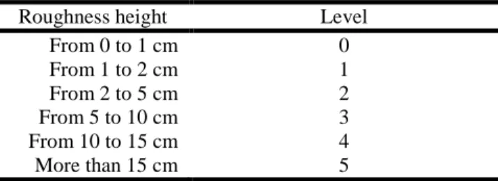
inspection during field mapping. Each of the two roughness indices are tagged using a six-level scale 15

(Table 1). Thus, two roughness attributes are recorded for each polygon. The polygons must also have 16

an attribute describing the tillage direction in degrees (from 0 to 179°). 17

2.1.2 Topography 18

The second mandatory layer is raster-type and represents the topography of the studied area. It is a 19

DEM. The common area between the DEM and the agricultural field polygons defines the largest area 20

that can be modeled by the ‘flow network’ module. To account for the edge effects caused by some 21

numerical treatments, a 5-cell buffer is added around the area defined by the agricultural field 22

polygons. 23

(7)

Version postprint

p

t

2.1.3 Preferential flow paths 1

The third layer is optional. It accounts for the preferential flow paths caused by objects such as the 2

headlands (i.e., the unplowed land at both ends of a field after the primary plowing: headlands are 3

usually plowed subsequently, across the primary plowing direction), open furrows (i.e., a long shallow 4

trench in the ground left in the middle of the field or between two fields after plowing), and roads. 5

This layer is vector-type with a line topology. Each line has attributes describing its hydrologic 6

behavior. Depending on these attributes, changes in the flow directions of the underlying cells will be 7

made, thereby modifying the flow network. 8

2.2 Computation of the flow network 9

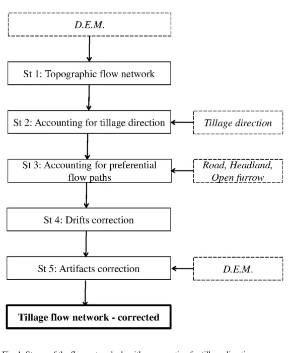
The successive stages of the algorithm are illustrated in Figure 1. 10

11

2.2.1 Stage 1 – Building the topographic flow model of flow directions 12

In a the Geographical Information System (GIS) software using square cell raster grids, one of eight 13

possible flow directions is assigned to each grid cell. Each of these eight possible directions leads to 14

one of the eight neighboring cells. The flow direction for the cell under inspection is computed from a 15

raster DEM representing the topography by selecting the neighboring cell with the steepest descent. 16

This generates a strictly convergent flow network (i.e., the flow of one cell is never routed to more 17

than one other cell). When applied to a DEM free of sinks, starting from any cell and following the 18

flow direction from cell to cell always leads to the edges of the studied area (the edges can be 19

identified by cells with a special value called ‘NODATA’). 20

The first stage consists of computing the topographic flow network. It is called the topographic flow 21

network because it is built by accounting for the topography only. This network is then used as a 22

reference to build the flow network that accounts for the manmade features, as described hereafter. 23

2.2.2 Stage 2 – Modifying the topographic flow network to account for tillage directions 24

In the cultivated fields, the flow directions are not always the topographic flow direction. The flow 25

directions can be modified following some rules described in Souchère et al. (1998). In locations with 26

large slope gradients, the actual flow directions are determined by the topography only, whereas in 27

(8)

Version postprint

p

t

locations with gentle slopes, the actual flow directions can be determined either by the topography or 1

by the direction of the tillage, depending on the soil surface roughness. 2

In fact, the tillage operations alter the surface roughness by making it anisotropic. As a consequence, 3

the tillage operations can create preferential flow directions. Some of the tillage operations create such 4

large roughness anisotropy that the flow will always follow the tillage direction. For example, the 5

ridging of potato fields creates a large roughness across the tillage direction but a low roughness along 6

the tillage direction. As a consequence, the flow is channeled by the ridges. 7

Souchère et al. (1998) assumed that the overland flow direction at a given location depends on two 8

major variables: the slope intensity, and the angle between the azimuths of the steepest slope and of 9

the tillage direction. To verify this assumption, they measured the slope with an Abney level and the 10

angle between the two directions with a compass on 60 plots. At the same time, the actual overland 11

flow direction was noted for each plot either by direct observation during rainstorms or by analyzing 12

the traces left by overland flow just after the event. 13

Ten observations demonstrated that if the difference between the roughness across and the roughness 14

along the tillage direction is greater than two levels (as defined in Table 1), the flow direction is 15

always the tillage direction. For the other fifty observations (i.e. if the roughness anisotropy is equal or 16

lower to two levels), the flow can be along the tillage direction or along the topographic slope. In this 17

case, the observations were ranked in two sub-populations corresponding to: (i) plots where the 18

observed overland flow follows predominantly the slope direction and (ii) plots where tillage imposes 19

the overland flow direction. Using these data, an analysis of the variance and a discriminant analysis 20

were performed using the two chosen variables – the slope intensity and the angle between the steepest 21

slope and the tillage direction – to produce a suitable procedure for automatically determining the 22

overland flow direction. 23

Souchère et al. (1998) used this discriminant function to categorize the grid cells into two sets: those 24

with a flow direction along the topographic slope and those with a flow direction along the tillage 25

direction. The discriminant function is: 26 03 . 3 45 . 5 6669 . 0 95 . 19 74 . 61 6646 . 0 − − − − = angleW slope Discrim (1) 27

(9)

Version postprint

p

t

with angleW the angle (in degree) between the tillage direction and the topographic slope aspect, and 1

slope the topographic slope gradient (in %).

2

The value Discrim is then used with a threshold equal to 0.1249 to assign the grid cells with the tillage 3

direction (Discrim > 0.1249) or to keep the direction of the topographic flow network computed in the 4

first stage described above (Discrim ≤ 0.1249). The statistical analysis of Souchère et al. (1998) 5

showed that 92% of the 50 test plots were correctly classified by the discriminant function, while the 6

wrongly classified plots had intermediate situations in terms of (1) the slope gradient and (2) the angle 7

between the tillage direction and the slope aspect. 8

After stage 2, there is a flow network accounting for tillage directions, but, resulting from the 9

limitation of flow to only height possible directions per cell, a bias (or drift) is present in the flow 10

directions. This will be corrected in stage 4 of the procedure. But before this correction takes place, the 11

preferential flow paths are included. 12

2.2.3 Stage 3 – Modifying the tillage flow network to account for preferential flow paths 13

If the user chooses to provide the optional layer describing the preferential flow paths, this information 14

is processed: 15

• In the headlands, the discriminant function (1) is used with the tillage direction inside the 16

headland. Typically, this tillage direction crosses the general tillage direction of the field but is 17

parallel to one of the field edges. 18

• For roads, the direction of the topography is kept. 19

• For open furrows, the flow direction is set to be downslope, along the open furrow. 20

As a result of this third stage, the new flow network accounts not only for tillage directions but also for 21

preferential flow paths. It now needs to be corrected from the drift. 22

2.2.4 Stage 4 – Cancellation of the drift in the tillage flow network 23

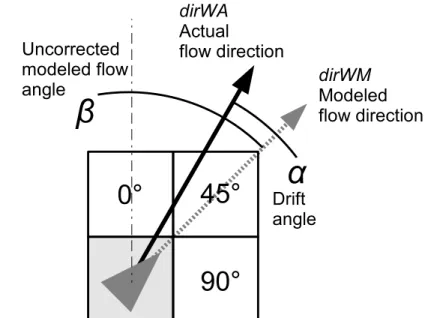
When tillage directions are translated into flow directions (at stage 2), drifts in the modeled flow 24

directions are introduced. The flow directions on square grids are set in 45° increments. The 25

intermediate directions cannot be modeled at the scale of a single grid cell. The drift causes a 26

misdirection of the flow (Fig. 2). The maximum drift angle is equal to 22.5°. This effect is especially 27

(10)

Version postprint

p

t

sensitive for long fields: the modeled flow directions will lead the flow to cross the field edge instead 1

of being parallel to it. This can lead to a misrepresentation of the flow network. Moreover, by 2

changing the contributing area at the watershed outlet, the drift can cause miscalculations of the 3

cumulated flow. 4

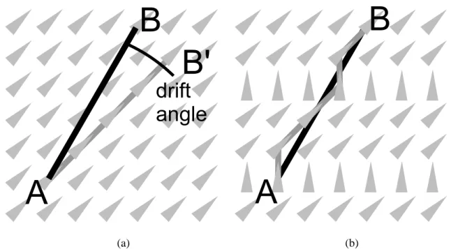
The effect is illustrated at the scale of several cells in Figure 3(a). The actual flow direction is along 5

AB, at the azimuth at 30°. By following the grey arrows, the flow network should lead from point A to 6

point B. However, with the grey arrows having an azimuth of 45°, they lead to point B’ instead. The 7

angle between AB and AB’ is equal to the drift angle. 8

To accound for the drift, the modeled tillage flow direction needs to be corrected at a constant interval 9

(every x columns or every y rows). The interval between the corrections is calculated based on 10

trigonometry. 11

We define the drift

α

as the angle between dirWA (the actual tillage direction) and dirWM (the 12

modeled flow direction before correction) (Fig. 2): 13 dirWM dirWA− =

α

(2) 14

α

ranges from -22.5° to 22.5°. 15

We define

β

as the modeled flow direction before correction.

β

takes one of the eight possible 16

directions (0°, 45°, 90°, etc.). 17

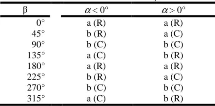
Depending on the case, the correction consists of applying one of the following two formulas: 18

α

β

/tan cos _(a) 19

α

β

/tan sin _(b) 20

Table 2 indicates the formula to be used depending on the values of

α

and

β

, and determines whether 21

the correction must be applied on an interval of rows (R) or columns (C). 22

The removal of the drift, by counterbalancing it at regular intervals, creates a better overall flow 23

direction (Fig. 3(b)). The tillage flow network after the drift cancellation follows the line AB. This 24

method of drift cancellation better models the tillage direction at the field scale. 25

(11)

Version postprint

p

t

2.2.5 Stage 5 – Removal of flow direction artifacts 1

The introduction of constrained flow directions in the topographic flow direction model generates 2

some artifacts. These artifacts are inconsistencies that make the flow network inappropriate for 3

hydrological processing. The computation of the flow accumulation requires first the definition of the 4

flow direction of all of the cells. The changes introduced by the tillage direction and the preferential 5

flow paths are made at the scale of the individual cells without considering the flow directions in the 6

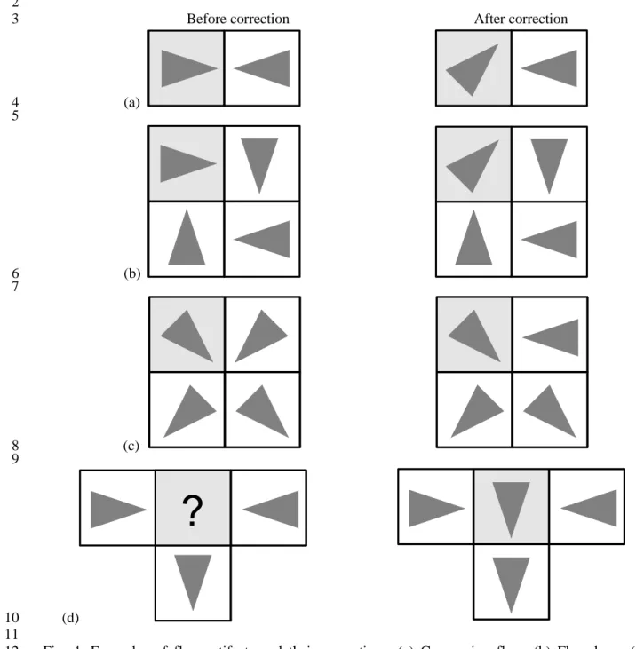
neighboring cells. This creates four kinds of artifacts: converging flows, flow loops, crossing flows, 7

and unspecified directions (Fig. 4 left). These artifacts need to be removed before the flow 8

accumulation can be computed properly (Fig. 4 right). All of these changes in flow directions are 9

made without taking into account the actual flow paths. 10

• Converging flows. Converging flows occur when two neighboring cells point to each other making

11

it impossible to define a downstream flow path (Fig. 4(a) left). The solution consists of changing 12

the flow direction of the current cell to switch it to the topographic direction (Fig. 4(a) right). 13

• Flow loops. Following a flow path that leads back to an already visited cell is considered a flow

14

loop (Fig. 4(b) left), again making it impossible to define a downstream flow path. Again, the 15

solution consists of changing the flow direction of the current cell to switch it to the topographic 16

direction (Fig. 4(b) right). 17

• Crossing flows. This type of artifact occurs when the direction of the neighboring cell (white

18

background in (Fig. 4(c) left)) is at 90° to the current cell (grey background). The solution consists 19

of changing the direction of the neighboring cell by 45° so that it now flows into the current cell 20

(Fig. 4(c) right). Doing so – instead of changing the current cell – ensures that no other crossing 21

flow is being created by the change. 22

• Unspecified directions. Unspecified directions can be created during the computation of the flow

23

directions when working within the open furrows. At stage 3, the modeling of the flow directions 24

within the open furrows is achieved by artificially increasing the altitudes of the cells surrounding 25

the furrows. Doing so ensures that the flow direction is identical to that of the underlying furrow. 26

But, as a consequence, when a furrow crosses a thalweg, a local minimum appears in the DEM, 27

(12)

Version postprint

p

t

causing a so-called ‘sink.’ Such a sink has the effect of disrupting the flow path network where it 1

should normally lead to the edge of the study area. The sink cells receive an unspecified flow 2

direction (Fig. 4(d) left). The solution to an unspecified direction again consists of switching it 3

back to the topographic flow direction. This causes the open furrow to overflow at the location of 4

the thalweg it crosses. Hence, this solution restores the usual behavior of an open furrow at the 5

field (Fig. 4(d) right). 6

The automatic procedure to remove artifacts is run twice in the ‘flow network’ module. During the 7

first run, the corrections are not applied to the cells labeled as open furrows. This avoids the creation 8

of crossing flows. In most of the cases, this solves the artifacts around the open furrows, except for the 9

unspecified directions. During the second run, all of the remaining artifacts are solved, including those 10

located in the open furrows. 11

2.3 Test watershed 12

The ‘flow network’ module was implemented in the “STREAM” watershed hydrologic modeling 13

software (Cerdan et al., 2002b). This section details how the tillage directions and associated 14

manmade features modify the flow network. The modeled flow network is compared to the actual flow 15

network. 16

2.3.1 Watershed description 17

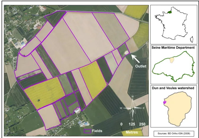
The watershed used to test the ‘flow network’ module is located in northern France, in the department 18

of Seine Maritime, in the commune of Blosseville (Fig. 5). The agricultural watershed has a surface 19

area of 87 hectares, with loamy soils sensitive to crusting. The lateral flows are mostly surface flows. 20

The village, located at the outlet of the watershed, has undergone significant damage caused by muddy 21

floods. To decrease the risk of flooding, a watershed management plan was set up. The STREAM 22

model was used to evaluate the effectiveness of the soil and water conservation practices. 23

2.3.2 Data requirements 24

Except for the DEM, the method has been designed for using data that do not require any specific 25

equipment (laser scanner, etc.) during the field data collection. A first field study was performed to 26

(13)

Version postprint

p

t

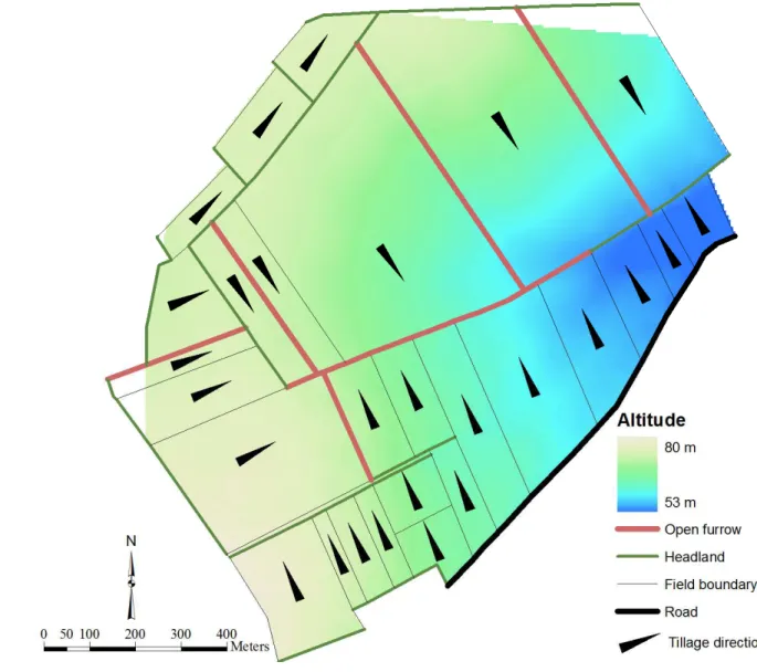
obtain, for each agricultural field, the information necessary to model the flow directions: tillage 1

direction, roughness along the tillage direction, roughness across the tillage direction, and location and 2

type of preferential flow paths (Fig. 6) or (Fig. 7). In less than two hours, these parameters could be 3

easily mapped by the visual inspection of all fields. It makes the use of the ‘flow network’ module 4

cost-effective. In addition, the formation of an operator is easy. The information needed to build the 5

DEM came from digitizing the contour lines of a topographic map and from a complementary survey 6

of topographic points. It had a horizontal resolution of 5 m. Altitudes were stored as floating-point 7

numbers. 8

This enables the prediction of soil surface characteristics could be deduced from information on crop 9

type, soil surface texture, and rainfall regimes (Delmas et al., 2012). This enables to predict soil 10

surface characteristics and their evolution during the cultivation season without further field study. 11

2.4 Validation 12

The computed flow networks are compared to the observed rill network. Erosion rills are a direct and 13

visible indication of flow directions inside a watershed. They were mapped using a theodolite. Given 14

the size of the catchment, they could be mapped on only part of the watershed. A thorough cell-to-cell 15

comparison of the actual versus predicted flow network would not have been possible because the 16

actual flow directions cannot be detected everywhere. 17

First, the validation is performed by a visual comparison of the computed flow networks with the 18

observed flow network. Then, to quantify the improvement induced by the proposed algorithm, the 19

following methodology is executed: 20

• The flow networks, refined as much as possible, are computed both from the topographic flow 21

network (TOPO) and the tillage flow network (TILL). The lines in the observed erosion network 22

(OBS) are cut into 5-meter-long segments corresponding to the DEM resolution. For each segment 23

of these 3 networks (TOPO, TILL, and OBS), the flow azimuth is computed (TOPOAZIM, 24

TILLAZIM, and OBSAZIM). For each segment in the observed network (OBS), the nearest 25

segment in both the topographic (TOPO) and the tillage (TILL) flow network is identified. This 26

allows attributing the nearest TOPOAZIM and TILLAZIM to the OBS segment. At this stage, for 27

(14)

Version postprint

p

t

each observed erosion line segment, its own azimuth, the azimuth of the topographic flow 1

network, and the azimuth of the tillage flow network are known. 2

• The absolute acute angle (gap angle) between the observed and the topographic network azimuth 3

is computed (TOPOGAP = modulo180(abs(OBSAZIM - TOPOAZIM))). The same is performed 4

with the tillage network azimuth (TILLGAP = modulo180(abs(OBSAZIM - TILLAZIM))). The 5

difference (Q) between these two angles (Q = TOPOGAP - TILLGAP) provides, for each 6

observed segment (OBS) considered a ground truth, an indication of the improvement in quality 7

obtained using the tillage flow network instead of the topographic flow network. A positive Q 8

value indicates a gain in quality, whereas a negative Q value indicates a loss in quality. The value 9

itself indicates the intensity of this gain/loss of quality. 10

3 Results and discussion

11

3.1 Model of the flow directions 12

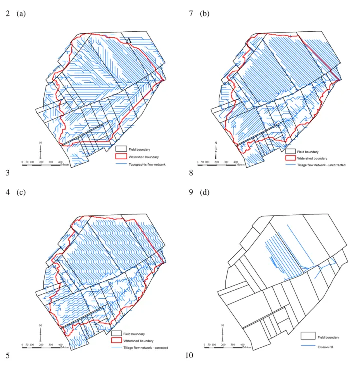
The first stage was to create the topographic flow network based on the DEM (Fig. 8(a)). 13

The second stage makes use of the discriminant function to define the cells where the flow is 14

controlled by the tillage direction. This stage also includes the effect of the preferential flow paths on 15

flow directions. According to the discriminant function, the tillage operations control a large part of 16

the flow directions inside the watershed (Fig. 9). In the northern part of the watershed, the tillage 17

operations define the flow direction in most of the agricultural fields. After this stage, the tillage flow 18

network shows a drift in the flow directions (Fig. 8(b)): in the northern part of the watershed, the flow 19

network crosses the field boundaries. If overland flow is modeled using this network, water will be 20

routed from one field to a sideway field, even if the tillage directions, which, at this location, should 21

control the flow direction, are parallel to the field boundaries (Fig. 7). This clearly illustrates the drift 22

of flow directions caused by the requirement for the flow directions to be along one of the eight 23

directions at the cell scale. The tillage operations on the northern fields have an actual direction of 24

145°. At the cell level, the closest direction is 135°. This caused the flow direction of 145° (south-east) 25

to be overstated among the flow directions in the uncorrected tillage flow network (Fig. 10). 26

(15)

Version postprint

p

t

To alleviate this problem, the drift-cancellation method is used to shift by 45° some of the cells with 1

the appropriate ratio. For the specific case of actual directions at 145°, some of the directions modeled 2

at 135° are shifted to the direction 180°. After drift cancellation, the number of flow directions 3

pointing at 135° is decreased in the corrected tillage flow network (Fig. 10). Simultaneously, the 4

number of directions at 180° is increased. After the removal of the flow direction artifacts, the new 5

network better accounts for the tillage directions and is consistent with the hydrologic uses (Fig. 8(c)): 6

the flow network remains parallel to the field boundaries instead of crossing them sideways. Taking 7

into account tillage operations and cancelling the drift also modified the watershed boundaries 8

(compare Fig. 8(a) and Fig. 8(c)): two fields located in A on Fig. 8(a) are now fully connected to the 9

outlet, which was not the case with the topographic model. This underlines also the need of using a 10

DEM covering an area larger than that of the study area. 11

3.2 Validity of the tillage flow network 12

The above section demonstrates that the tillage flow network sensibly incorporates manmade features 13

in an agricultural watershed. The validity of the tillage flow network can be further estimated by a 14

comparison with the actual flow network. 15

The actual flow network is the network of the observed rills (Fig. 8(d)). The visual comparison of 16

Fig. 8(a) with Fig. 8(d) shows that the topographic network does not account well for the actual flow 17

network. The same exercise with Figure 8(c) or Figure 8(d) provides a better match of the corrected 18

tillage network with the actual flow network. 19

Figure 11 represents the frequency distribution of Q values. Out of the 1240 observed segments, the 20

proposed algorithm modified 587 segments (47%) by more than 1°. Among these, 455 segments 21

(77%) have a positive Q. Hence, most of flow directions modified by the proposed algorithms led to 22

an improved flow direction. This clearly demonstrates that taking into account tillage directions 23

improves the quality of the flow network. 24

(16)

Version postprint

p

t

4. Conclusions and perspectives

1

In an agricultural context, and for a watershed with gentle slopes, the surface flow network is largely 2

affected by agricultural practices. The flow network computed from the DEM solely does not match 3

the actual flow network with enough accuracy to allow for a good modeling of the overland flow and 4

soil erosion. 5

The topographic network model can be improved with information about the tillage operations and 6

preferential flow paths (such as open furrows). Including this information introduces some artifacts in 7

the flow directions. These artifacts must be corrected to create a flow network usable for hydrologic 8

purposes. The most important artifact is a drift in the flow direction everywhere the flow direction is 9

controlled by the tillage operations. A method to cancel this drift is proposed. It should be applicable 10

to most of the cell-based flow networks. The automatic procedures to correct other artifacts are also 11

presented. 12

The comparison among the topographic flow network, the corrected tillage flow network, and the 13

observed erosion marks shows that the described method matches successfully the actual flow 14

network. It also shows that using only the topography to account for the flow directions leads to large 15

discrepancies in the agricultural areas. 16

The proposed method could be further improved. Currently, only the convergent flows are modeled 17

because we are using a “single flow direction” algorithm. However, some field observations show that 18

divergent flow can also occur, especially in sedimentation areas. Another flow network algorithm, 19

such as the “multiple flow algorithm” of Quinn et al. (1991), could be implemented to account for this 20

feature. The visual observations also showed that the flow directions can change depending on the 21

water flux. For a small water flux, the flow depth is low and the flow direction is along the tillage 22

direction. However, for a larger water flux, the flow depth increases and the furrows can overflow, 23

increasing the flow to the topographic slope aspect. This phenomenon can occur during a single rain 24

event and is not accounted for in the current method. No alternative method is currently available. 25

New research will be needed to address this issue. However, future studies will have to face the 26

(17)

Version postprint

p

t

difficulty of the distributed water-flux measurements inside an agricultural field. Taking changes in 1

flow depth into account would lead to a network able to evolve during a rainfall event. 2

Acknowledgements

3

This work was funded by a GESSOL research grant from the French Ministry of Environment. This 4

support is gratefully acknowledged. It was also supported by the ANR VMC program within the 5

framework of the MESOEROS21 and LANDSOIL projects. The authors are grateful to the two 6

anonymous reviewers who helped improve the manuscript. 7

References

8

Auzet, A.V., Boiffin, J., Ludwig, B., 1995. Concentrated flow erosion in cultivated catchments: 9

influence of soil surface state. Earth Surface Processes and Landforms 20, 759–767. 10

Bailly, J.S., Lagacherie, P., Millier, C., Puech, C., Kosuth, P., 2008. Agrarian landscapes linear 11

features detection from LiDAR: application to artificial drainage networks. International Journal of 12

Remote Sensing 29, 3489–3508. 13

Bingner, R.L., Theurer, F.D., 2007. AGNPS: AGricultural Non-Point Source Pollution Model. 14

Available online at: http://www.ars.usda.gov/Research/docs.htm?docid=5199 (accessed on 11 July 15

2012). 16

Boiffin, J., Papy, F., Eimberck, M., 1988. Influence of cropping systems on the risk of concentrated 17

flow erosion. I. ─ Analysis of the conditions for initiating erosion [in French]. Agronomie 8, 663– 18

673. 19

Cerdan, O., Le Bissonnais, Y., Souchère, V., Martin, P., Lecomte, V., 2002a. Sediment concentration 20

in interrill flow: Interactions between soil surface conditions, vegetation and rainfall. Earth Surface 21

Processes and Landforms 27, 193–205. 22

Cerdan, O., Souchère, V., Lecomte, V., Couturier, A., Le Bissonnais, Y., 2002b. Incorporating soil 23

surface crusting processes in an expert-based runoff model: STREAM (Sealing and Transfer by 24

Runoff and Erosion related to Agricultural Management). Catena 46, 189–205. 25

(18)

Version postprint

p

t

Delmas, M., Pak, L., Cerdan, O., Souchère, V., Le Bissonnais, Y., Couturier, A., Sorel, L., 2012. 1

Water and sediment transfer from the field to the river in an agricultural catchment of the European 2

Loess belt. Journal of Hydrology 420-421, 255–263. 3

Desmet, P.J.J., Govers, G., 1997. Two-dimensional modelling of the within-field variation in rill and 4

gully geometry and location related to topography. Catena 29, 283–306. 5

Flanagan, D.C., Nearing, M.A., 1995. USDA - Water Erosion Prediction Project. Hillslope profile and 6

watershed model documentation. Report n°10, USDA-ARS, National Soil Erosion Research 7

Laboratory, West Lafayette, Indiana, Available online at: 8

http://www.ars.usda.gov/research/publications/publications.htm?seq_no_115=64035 (accessed on 9

11 July 2012). 10

Furlan, A., Poussin J.C., Mailhol, J.C., Le Bissonnais, Y., Gumiere, S.J., 2012. Designing 11

management options to reduce surface runoff and sediment yield with farmers: An experiment in 12

South-Western France. Journal of Environmental Management 96, 74–85. 13

Govers, G., Takken, I., Helming, K., 2000. Soil roughness and overland flow. Agronomie 20, 131– 14

146. 15

Le Bissonnais, Y., Gascuel-Odoux, C., 1998. Water erosion of cultivated soils in temperate area [in 16

French]. In: Stengel, P., Gelin, S., (Eds.), Sol: interface fragile. INRA Edition, Paris, pp. 129–144. 17

Le Bissonnais, Y., Cerdan, O., Lecomte, V., Benkhadra, H., Souchère, V., Martin, P., 2005. 18

Variability of soil surface characteristics influencing runoff and interrill erosion. Catena 62, 111– 19

124. 20

Ludwig, B., Boiffin, J., Chadoeuf, J., Auzet, A.V., 1995. Hydrological structure and erosion damage 21

caused by concentrated flow in cultivated catchments. Catena 25, 227–252. 22

Morgan, R.P.C., Quinton, J.N., Smith, R.E., Govers, G., Poesen, J.W.A., Auerswald, K., Chisci, G., 23

Torri, D., Styczen, M.E., 1998. The European Soil Eosion Model (EUROSEM): a dynamic 24

approach for predicting sediment transport from fields and small catchments. Earth Surface 25

Processes and Landforms 23, 527–544. 26

O’Callaghan, J.F., Mark, D.M., 1984. The extraction of drainage networks from digital elevation data. 27

Computer Vision, Graphics, and Image Processing 28, 323–344. 28

(19)

Version postprint

p

t

Orlandini, S., Moretti, G., Franchini, M., 2003. Path-based methods for the determination of 1

nondispersive drainage directions in grid-based digital elevation models. Water Resources 2

Research 39, 1144. 3

Orlandini, S., Tarolli, P., Moretti, G., Dalla Fontana, G., 2011. On the prediction of channel heads in a 4

complex alpine terrain using gridded elevation data, Water Resources Research 47, W02538, doi: 5

10.1029/2010WR009648. 6

Papy, F., Boiffin, J., 1989. The use of farming systems for the control of runoff and erosion. In Soil 7

Erosion Protection Measures in Europe. Proceedings of the European Community. Workshop on 8

Soil Erosion Protection, Freising, Germany, pp. 29–38. 9

Quinn, P., Beven, K., Chevallier, P., Planchon, O., 1991. The prediction of hillslope flow paths for 10

distributed hydrological modelling using digital terrain models Hydrological Processes 5, 59–79. 11

Souchère, V., King, D., Daroussin, J., Papy, F., Capillon, A., 1998. Effect of tillage on runoff 12

direction: consequences on runoff contributing area within agricultural catchments. Journal of 13

Hydrology 206, 256–267. 14

Souchère, V., Cerdan, O., Dubreuil, N., Le Bissonnais, Y., King, C. 2005. Modelling the impact of 15

agri-environmental scenarios on runoff in a cultivated catchment (Normandy, France). Catena 61, 16

229–240. 17

Tarboton, D.G., 1997. A new method for the determination of flow directions and upslope areas in 18

grid digital elevation models. Water Resources Research 33, 309–319. 19

Takken, I., Govers, G., Jetten, V., Nachtergaele, L., Steegen, A., Poesen, J., 2001. Effects of tillage on 20

runoff and erosion patterns. Soil & Tillage Research 61, 55–60. 21

Takken, I., Govers, G., Jetten, V., Nachtergaele, J., Steegen, A., Poesen, J., 2005. The influence of 22

both process descriptions and runoff patterns on predictions from a spatially distributed soil erosion 23

model. Earth Surface Processes and Landforms 30, 213–229. 24

Thorne, C.R., Zevenbergen, L.W., 1990. Prediction of ephemeral gully erosion on cropland in the 25

south-eastern United States. In: Boardman, J., Foster, D.L., Dearing, J.A. (Eds.), Soil Erosion on 26

Agricultural Land. Wiley, Chichester, pp. 447–460. 27

(20)

Version postprint

p

t

1

Table 1 - Roughness heights and corresponding levels Roughness height Level

From 0 to 1 cm 0 From 1 to 2 cm 1 From 2 to 5 cm 2 From 5 to 10 cm 3 From 10 to 15 cm 4 More than 15 cm 5 2

(21)

Version postprint

p

t

1

Table 2. Drift correction to be applied depending on the drift angle α and the topographic flow direction

modeled before correction β. β α < 0° α > 0° 0° a (R) a (R) 45° b (R) a (C) 90° b (C) b (C) 135° a (C) b (R) 180° a (R) a (R) 225° b (R) a (C) 270° b (C) b (C) 315° a (C) b (R)

Note: ‘a’ and ‘b’ refer to the formula numbers in the text.

2

‘C’ (‘R’) means that the correction has to be applied at a

3

given interval along the ‘columns’ (‘rows’)

4 5

(22)

Version postprint

p

t

List of figures

1

Fig. 1. Stages of the flow network algorithm accounting for tillage directions. 2

Fig. 2. Drift and drift angle. At the scale of a grid cell, the flow direction does not necessarily match 3

the actual flow direction. β represents the modeled flow direction. The drift angle α between the 4

modeled and the actual directions can be as great as 22.5°. 5

Fig. 3. Drift and its correction. The actual flow travels from point A to point B. (a) The drift causes the 6

flow to travel from point A to point B’. (b) The drift correction consists of tilting the flow direction at 7

regular intervals. It restores a general flow direction matching the actual flow direction. 8

Fig. 4. Examples of flow artifacts and their corrections. (a) Converging flow, (b) Flow loop, (c) 9

Crossing flow, (d) Unspecified flow direction. The cell under consideration has a grey background. 10

Fig. 5. Location map of the study area. 11

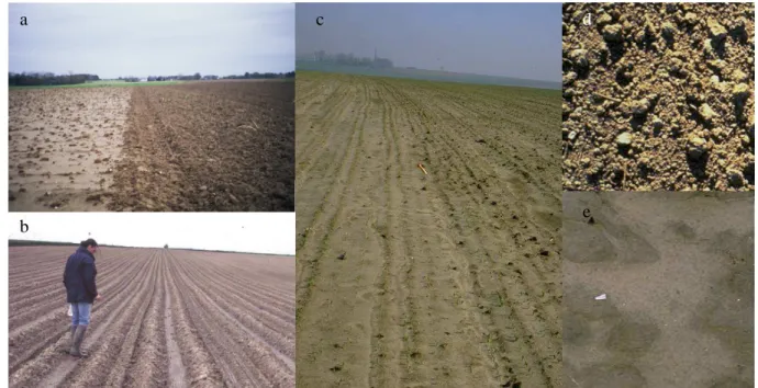
Fig. 6. Effects of the tillage operations on sealing, roughness, and surface runoff. (a) Crusted surface 12

on the left, tilled on the right. (b) Tilled field with deep furrows. (c) crusted furrows. (d) uncrusted 13

seedbed. (e) structural and sedimentary crusts. 14

Fig. 7. Data used by the ‘flow network’ module. 15

Fig. 8. Comparison of computed and observed flow networks. (a) Topographic flow model, based on 16

the Digital Elevation Model only. (b) Tillage flow network before the correction of the drift. (c) 17

Tillage flow network after the correction of the drift. (d) Erosion rill showing the actual flow direction 18

as observed in the field. 19

Fig. 9. Effect of the tillage and topography on flow directions. The flow can either follow the 20

topographic slope directions (light tone/brown color) or the tillage directions (dark tone/green color). 21

Fig. 10. Distribution of the flow directions for the computed flow networks. 22

Fig. 11. Frequency distribution of the Q values. A positive Q value indicates a gain in quality brought 23

by the proposed algorithm, whereas a negative Q value indicates a loss in quality. 24

(23)

Version postprint

p

t

1

2

Fig. 1. Stages of the flow network algorithm accounting for tillage directions. 3

(24)

Version postprint

p

t

1

2

Fig. 2. Drift and drift angle. At the scale of a grid cell, the flow direction does not necessarily match 3

the actual flow direction. β represents the modeled flow direction. The drift angle α between the 4

modeled and the actual directions can be as great as 22.5°. 5

6 7

(25)

Version postprint

p

t

Version définitive du manuscrit publié dans / Final version of the manuscript published in : Geomorphology, 2013, 183, 120-129 http://dx.doi.org/10.1016/j.geomorph.2012.07.025 1 2 (a) (b) 3

Fig. 3. Drift and its correction. The actual flow travels from point A to point B. (a) The drift causes the 4

flow to travel from point A to point B’. (b) The drift correction consists of tilting the flow direction at 5

regular intervals. It restores a general flow direction matching the actual flow direction. 6

(26)

Version postprint

p

t

1 2

Before correction After correction 3 (a) 4 5 (b) 6 7 (c) 8 9 (d) 10 11

Fig. 4. Examples of flow artifacts and their corrections. (a) Converging flow, (b) Flow loop, (c) 12

Crossing flow, (d) Unspecified flow direction. The cell under consideration has a grey background. 13

(27)

Version postprint

p

t

1

2

Fig. 5. Location map of the study area. 3

(28)

Version postprint

p

t

1

2

Fig. 6. Effects of the tillage operations on sealing, roughness, and surface runoff. (a) Crusted surface 3

on the left, tilled on the right. (b) Tilled field with deep furrows. (c) crusted furrows. (d) uncrusted 4

seedbed. (e) structural and sedimentary crusts. 5 6 a b c d e

(29)

Version postprint

p

t

1

2

Fig. 7. Data used by the ‘flow network’ module. 3

(30)

Version postprint

p

t

Version définitive du manuscrit publié dans / Final version of the manuscript published in : Geomorphology, 2013, 183, 120-129 http://dx.doi.org/10.1016/j.geomorph.2012.07.025 1 (a) 2 3 (c) 4 5 6 (b) 7 8 (d) 9 10 11

Fig. 8. Comparison of computed and observed flow networks. (a) Topographic flow model, based on 12

the Digital Elevation Model only. (b) Tillage flow network before the correction of the drift. (c) 13

Tillage flow network after the correction of the drift. (d) Erosion rill showing the actual flow direction 14

as observed in the field. 15

16

(31)

Version postprint

p

t

1

2 3

Fig. 9. Effect of the tillage and topography on flow directions. The flow can either follow the 4

topographic slope directions (light tone/brown color) or the tillage directions (dark tone/green color). 5

(32)

Version postprint

p

t

1

North-West North North-East East South-East South South-West West

0 10 20 30 40 50 Frequency (%)

Topographic flow network

Tillage flow network (uncorrected) Tillage flow network (corrected)

2

Fig. 10. Distribution of the flow directions for the computed flow networks. 3

(33)

Version postprint

p

t

1

2

Fig. 11. Frequency distribution of the Q values. A positive Q value indicates a gain in quality brought 3

by the proposed algorithm, whereas a negative Q value indicates a loss in quality. 4