Analysis and design of transonic cascades with splitter vanes

(1)

3 90803 OOL66926~ 8

ANALYSIS AND DESIGN OF TRANSONIC

CASCADES WITH SPLITTER VANES

by

H.H. Youngren

GTL Report #203

rJ778 .M41 .G24

March 1991

(2)

ANALYSIS AND DESIGN OF TRANSONIC

CASCADES WITH SPLITTER VANES

by

H.H. Youngren

GTL Report

#203

March 1991

This research was supported by the Air Force Office of Scientific Research, Grant

AFOSR-89-0373, with Captain Henry E. Helin as Program Manager and Dr. Arthur J. Wennerstrom as

Technical Monitor.

(3)

Analysis and Design of Transonic Cascades

with Splitter Vanes

by

Harold Hayes Youngren

A new computational method, MISES, is developed for turbomachinery design and

analysis applications. The method is based on the fully coupled viscous /inviscid method,

ISES, and is applicable to blade-to-blade analysis of axial fan and compressor stator or

rotors with optional splitter vanes. Quasi-three dimensional effects for stream surface radius, streamtube thickness and wheel rotation may be included. The flow is modeled with the steady Euler equations and the integral boundary layer equations. A robust Newton-Raphson method is used to solve the coupled non-linear system of equations, requiring only several minutes for solution on a typical workstation. Design options are implemented for either single surface or camber redesign.

The method is exercised by comparison with transonic cascade tests to validate the quasi-three-dimensional formulation. The results show excellent correlation to measured pressure distributions and loss levels. The multiple blade capability is demonstrated by comparison to test data for a supersonic cascade with splitter vane. New splitter vane configurations for improving the performance of the supersonic cascade are explored, resulting in large increases in turning and reduced loss.

(4)

Acknowledgements

This all started when I returned to MIT in 1987 to work on the Daedalus project and

to get a degree or two on the side... The former effort came off pretty much on schedule, give or take a crashed airplane or so. The latter effort ended up taking somewhat longer than I had anticipated...

I would first and foremost like to thank Mark Drela, thesis supervisor and long time

friend and airplane hacker, Newton whiz-extraordinaire, for all the help and fun along the way. His support on many fronts has made things easier. Also thanks to Mike Giles, co-whiz and friend, for ideas and help with his UNSFLO program.

I would also like to acknowledge the patience and persistence of Professors Witmer

and Markey for helping me back into the academic world of MIT after a long hiatus at Lockheed. Thanks.

The gang at the CFDL has been a source of support, entertainment and good com-pany. Thanks to you all, especially Sandy and Gerd my erstwhile climbing partners, Dana, Dave2, Phil2, Kousuke, Tom(the cartoonist), Peter, Andre, Helene, Missy, Ling and Bob Haimes. The special award for office-mate-beyond-the-call-of-duty goes to Eric Gaidos who tolerated my endless hackery on his computer terminal with an out of this world attitude...

Thanks especially to my family - Susan, Peter, Beth and my mother who have all come to think that this madness would never end. Finally, I would like to thank Cheryl, who has been patient and understanding beyond all reckoning with this compulsion to leave California (God's country) and return to Bean Town. Its time to go back.

This research was supported by the Air Force Office of Scientific Research Grant

AFSOR-89-0373, with Captain Henry E. Helin as Program Manager and Dr. Arthur J.

(5)

4.4.2 Computational Model . . . . 4.4.3 AVDR Effects . . . . 4.4.4 Pressure Comparison . . . . 57 59 61 62 62 64 . . . . 65 . . . . 65 . . . . 67 . . . . 6 7 . . . . 6 7 . . . . 69 . . . . 73 . . . . 73 . . . . 77 . . . . 78 . . . . 79 . . . . 80 . . . . 84

(8)

4.5 Convergence of Newton Solution . . . .9

5 Results - Design Applications 5.1 ARL Cascade w/o Splitter ... 5.2 Splitter Vane -Background ... 5.3 Splitter Vane Circumferential Position 5.4 Overview of ARL Cascade Flow Field 5.5 Modal Re-design of ARL Cascade . . . . 5.6 Alternate Design Directions . . . . 5.6.1 Splitter Vane Rotation . . . . 5.6.2 Short Chord Splitter Vane . . . . 5.6.3 Splitter Vane Axial Position . . . 5.6.4 Tandem Splitter Vane . . . . 94 . . . . 94 . . . . 9 6 . . . . 9 6 . . . . 9 9 . . . . 100 . . . . 103 . . . . 103 . . . . 104 . . . . 106 . . . . 108

6 Conclusions and Recommendations

6.1 Test Cases... ...

6.2 Splitter Vane Optimization . . . .

6.3 Recommendations for Further Work . . . .

6.4 Characteristics of Ill-posed Boundary Conditions . . . .

A Development of Quasi-3D Euler Method

111 112 112 113 114 115 90

(9)

A.1 Coordinate System .1 A.2 A.3 A.4 A.5 A.6 A.7

A.5.4 S and N Momentum Equations .

A.5.5 Upwinding Scheme . . . .

A.5.6 Reduced N-Momentum Equation

Energy Equation . . . . Linearization of Equations . . . . Euler Equations . . . . Conservation Cell . . . . Continuity Equation . . . . Momentum Equation . . . .

A.5.1 Pressure Terms . . .

A.5.2 Flux Terms . . . . .

A.5.3 Rotational Forces . .

B Development of Quasi-3D Boundary Layer

B.1 Background -2D Boundary Layer . . . .

B.2 Quasi-3D Boundary Layer . . . .

B.2.1 Inviscid/ Viscous Coupling . . . .

C Cascade Loss Calculation

C.1 Inviscid Loss Calculation. . . . .

. . . . 116 ... 117 . . . ... . . . . 120 . . . . 121 . . . . 121 . . . . 123 . . . . 125 . . . . 127 . . . . 128 . . . . 129 . . . . 130 . . . . 131 132 132 134 135 136 137 115

(10)

C.2

C.3

C.4

Viscous Loss Calculation . . . .

Loss at Uniform Exit Condition . . . .

Loss Sensitivity Calculation . . . .

137

139

141

D Matrices and Linear System Solution 144

D.1 Newton System . . . . 144

D.1.1 Jacobian Matrix . . . . 146

D.1.2 Block Structure . . . . 147

D.1.3 Matrix Blocks with Boundary Layer . . . . 149

D.2 Solution of Linear System . . . . 151

D.2.1 Solution Method for Choked Flow . . . . 152

D.3 Multiple Blades . . . . 154

D.3.1 Block Structure for Multiple blades . . . . 155

D.3.2 Multiple Blade Choked Flow Solution . . . . 157

D.4 Offset-Periodic Matrix . . . . 158

D.4.1 Offset Block Structure . . . . 160

D.4.2 Offset Matrix Solution . . . . 160

(11)

List of Figures

1.1 Blade sections for ARL cascade with splitter vane. . . . .

1.2 Effect of splitter vane on pressure distributions for ARL cascade...

2.1 Cascade coordinate system . . . .

2.2 Blade-to-blade flow on a stream surface of revolution . . . .

2.3 Meridional (r-z) plane for defining stream surfaces . . . .

2.4 Equivalent inviscid flow defined by BL displacement thickness . . . .

2.5 Variation of mass flow with Mach number . . . .

2.6 Supersonic/axially-subsonic inflow for cascade, showing inlet wave system

2.7 Characteristic families for local angle 0 and Mach . . . .

3.1 Streamline grid system for discrete Euler equations. . . . .

3.2 Conservation cell and variable locations. . . . .

3.3 Boundary conditions on domain boundaries. . . . .

3.4 Domain of dependence for S-momentum and N-momentum equations. .

3.5 Boundary conditions for viscous coupling. . . . .

3.6 Mode shapes and design modes for geometric perturbations. . . . .

23 24 26 27 27 29 32 34 35 39 39 41 45 49 50

(12)

3.7 Cascade with splitter blade, showing stagnation lines. . . . . 52

3.8 Grid arrangement for multiple blades. . . . . 52

3.9 Design modes for splitter movement and rotation . . . . . 54

3.10 Dispersion effects at shock for skewed grid. . . . . 57

3.11 Supersonic odd-even instability for skewed grids. . . . . 58

3.12 Grid and Mach contours for blunt LE blade, = 500, M = 1.3 . . . . . 58

3.13 Layout of offset-periodic grid. . . . . 59

3.14 Pressure distribution for supersonic cascade with offset-periodic grid. . . 60

3.15 Grid and Mach contours for cascade with offset-periodic grid. . . . . 60

3.16 Arrangement of off-diagonal periodicity terms for offset grid. . . . . 61

4.1 UTRC test case grid 132x20 . . . . 66

4.2 Pressure distribution for UTRC Build I: M = 0.113,,81 = 38.0', AVDR = 1.023... ... 66

4.3 Blade section for DFVLR tests . . . . 68

4.4 Offset-periodic 220x20 grid for DFVLR cases . . . . 69

4.5 AVDR Effect on DFVLR blade: M = 0.82, 01 = 58.50.. . . . . 70

4.6 AVDR Effect on DFVLR blade: M = 0.92, ,1 = 58.5 . . . . 71

4.7 AVDR Effect on DFVLR blade: M = 1.03, #3 = 58.50 . . . . 72

(13)

4.9 Comparison of predicted and measured loss for DFVLR cascade . . . . . 73

4.10 DFVLR blade: Al = 1.023, i3 = 56.8', AVDR = 1.092 . . . . 75

4.11 Mach contours for DFVLR blade, M = 1.023, contour interval 0.05 . . . 75

4.12 DFVLR blade: M = 1.086, 31 = 58.5', AVDR = 1.184 . . . . 76

4.13 Mach contours for DFVLR blade, M = 1.086, contour interval 0.05 . . . 76

4.14 Blade and splitter vane for ARL cascade . . . . 77

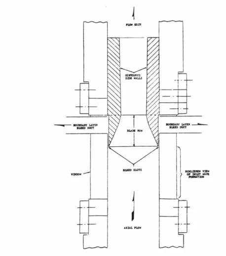
4.15 Top view of ARL test section showing sidewall contraction . . . . 79

4.16 Offset-periodic 220x20 grid for ARL cases . . . . 80

4.17 Streamtube width for ARL cascade at metal-metal and 109% AVDR. . . 81

4.18 Effect of AVDR on exit angle for ARL cascade . . . . 82

4.19 Effect of AVDR on total and viscous loss for ARL cascade . . . . 82

4.20 Pressure distribution for AVDR = 1.95. . . . . 83

4.21 Pressure distribution for AVDR = 2.295. . . . . 83

4.22 Surface pressures for ARL with splitter, P2/PI = 2.034, 109% AVDR. . 85 4.23 Mach contours for ARL cascade, contour interval 0.05, P2/P1 = 2.034 . 85 4.24 Surface pressures for ARL blades, P2/P1 = 1.741, 109% AVDR. . . . . . 86

4.25 Mach contours for ARL cascade, contour interval 0.05, P2/PI = 1.741 . 86 4.26 Effect of pressure ratio on exit angle for ARL cascade 109% AVDR. . . 87

(14)

4.28 Thickening of blade boundary layer with sidewall boundary layer fluid. . 89

4.29 Convergence of Max density change for analysis cases . . . . 91

4.30 Convergence of loss for analysis cases . . . . 91

4.31 Convergence of Max density change for ARL Splitter with initialized flow field . . . . 93

5.1 Pressure distribution for main blade at P2/p1 = 1.93, 109% AVDR . . . . 95

5.2 Pressure distribution for main blade at P2/P1 = 2.03, 109% AVDR . . . . 95

5.3 Effect of splitter vane circumferential position on loss . . . . 97

5.4 Pressure distribution for ARL cascade with 44% splitter position . . . . 98

5.5 Pressure distribution for ARL cascade with 56% splitter position . . . . 98

5.6 Redesigned blade section compared to original ARL blades. . . . . 101

5.7 Surface pressures for redesigned ARL cascade at P2/PI = 1.93 . . . . 102

5.8 Surface pressures for ARL cascade at +30 splitter incidence . . . . 104

5.9 Surface pressures for shortened chord splitter at P2/p1 = 1.93 . . . . 105

5.10 Surface pressures for original splitter at P2/P1 = 1.93 . . . . 105

5.11 Surface pressures for ARL cascade at p2/p1 = 2.03 . . . . 107

5.12 Surface pressures for ARL cascade with splitter moved +0.20 downstream 107 5.13 Tandem configuration with 70% chord splitter vane. . . . . 109

(15)

5.15 Mach contours for 70% chord tandem splitter . . . .1

6.1 Characteristic behavior for ill-posed boundary conditions. . . . . 114

A.1 Conservation cell on nodal grid . . . . 117

A.2 Conservation cell and edge vectors . . . . 118

A.3 Conservation cell . . . . 118

A.4 Flux terms from circumferential displacement of velocity vectors . . . . 123

A.5 Pressures on neighboring streamtubes . . . . 129

D.1 Newton variables for discrete Euler equations. . . . . 144

D.2 Domain of dependence for S-momentum and N-momentum equations. 145 D.3 Structure of Ai and Ci blocks. . . . . 147

D.4 Structure of Zi and Bi blocks. . . . . 147

D.5 Structure of inlet blocks. . . . . 148

D.6 Structure of exit blocks. . . . . 148

D.7 Domain of dependence of boundary layer unknowns, from Drela. . . . . 149

D.8 Shifting of S-momentum equation rows for choked solver. . . . . 153

D.9 Layout of streamtubes and streamlines in multiple blade grid . . . . 154

D.10 Domain of dependence for reduced N-momentum equation across stag-nation stream line. . . . . 155

D.11 Offset-periodic inlet geometry and indexing. . . . . 158

(16)

(17)

List of Tables

Discrete boundary conditions on domain edges. . . . .

Direct constraint equations for global DOF's. . . . .

5.1 Stepwise modal redesign of ARL cascade with splitter vane. .

5.2 Effect of splitter rotation, P2!PI = 1.93, 109% AVDR. . . . . .

5.3 Effect of splitter axial position, P2/Pl = 2.03, 109% AVDR. . .

C.1

Loss as a function of outlet length . . . .

. . . . . 100 . . . . . 103 . . . . . 106 139 3.1 3.2 . . . 42 . . . 47

(18)

a A,, AVDR b B B Cir C ,,, C, Dilo,., D,.of h H I IJ i".U i1i M/ 1 in', 0 fnj ft n An N

Nomenclature

speed of sound

quasi-normal face area vectors normal area

axial velocity density ratio P2q2 pt qi

streamtube width

streamwise face area vectors chord

inlet characteristic variable pressure coefficient

P,

specific heats

global movement modes for intermediate blades force vector

geometric mode enthalpy

BL shape factor rothalpy

streamwise offset on

j

1 streamline for offset grid streamwise and quasi-normal indices

unit vectors

maximum grid indices Mach number

local streamwise and circumferential coordinates total mass flow

mass flow in streamtube

j

geometric mode amplitude streamline normal coordinate gap between streamline and wall quasi-normal area vector

(19)

p pressure, pressure on quasi-normal face

ql velocity vector

q speed

r radius

RI) Reynolds number

streamwise direction vector

s boundary layer arc-length, components of streamwise vector S7,11,7 s,, inlet and outlet slopes

S streamwise area vector

T temperature

u speed in boundary layer

A V cell volume

X x direction, also m' coordinate

y y direction, also circumferential coordinate

z axial coordinate

flow angle change

V* boundary layer displacement thickness ratio of specific heats c,/c,.

A,

y first and second-order dissipation coefficients

V Prandtl-Meyer function

W non-dimensionalized loss parameter

11 rotational velocity

11+, i- pressures on streamline faces

p density

7' shear

0 BL momentum thickness

(20)

Superscripts:

()

averaged quantity () dimensional quantity

( )

vector

(^)

unit vector )+ 'upper' streamline

(

) 'lower' streamline Subscripts:

( )o

stagnation quantities

( )

inlet quantities, conservation cell node index

(

)2 exit quantities, conservation cell node index

(

):3

mixed-out quantities, conservation cell node index

(

) edge (outer)

(

);,

inner, outer stream surface face

( ),,,,

inlet quantity

(

),( 7n

isentropic

(

), leading edge, trailing edge

(

),... mean line

(

),,; reference quantity (at r = 0)

(

) ,specified quantity

(21)

Chapter 1 Introduction

This thesis will present a new computational method, MISES', which extends the fully coupled viscous/inviscid method, ISES, for application to quasi-three-dimensional cas-cade design. This method is intended for use as a tool for compressor cascas-cade design and analysis and for blade-to-blade design of axial stators and rotors.

The viscous flow is modeled using the steady Euler equations and integral boundary layer equations solved with a Newton-Raphson technique, the approach used in the

ISES code of Giles and Drela [1]. This has several advantages for design applications -accuracy, speed and a robust inverse design capability. Primarily, it is the speed that makes this approach attractive for design - a typical case is solved in 3-10 Newton cycles, a matter of minutes on a fast workstation. The accuracy also has a strong influence on the design process - the drag predictions from ISES are sufficiently good that they can be reliably used by a designer to optimize an airfoil at both on-design and off-design conditions, using wind tunnel testing only to verify the computational predictions. Although blade-to-blade design for turbomachinery is similar to the isolated airfoil design problem, there are additional difficulties in solving the viscous/inviscid governing equations, which are strongly coupled for transonic cascades. A design method for turbomachinery requires accurate loss prediction for strong shocks and for separated

flows.

This work also focuses on the analysis and design of cascades with multiple blades, specifically splitter vanes. These are introduced to reduce loss and increase turning

by changing the distribution of blade loading. They also increase blockage and can

increase viscous losses. This thesis addresses some of the design issues for multiple

(22)

blade cascades, focusing on the optimization of the splitter vane in a highly loaded supersonic cascade.

1.1 Motivation and Background

Improved levels of performance from gas turbine engines have motivated designers to place increasing reliance on computational techniques in the design process. This is especially true as blade loadings in compressors and turbines are increased and higher levels of refinement in design are attained. Unlike typical external aerodynamic design problems, where the design is driven to virtually eliminate strong non-linear flow effects, the interacting compressible and viscous effects in cascades lead to complex flows that frequently involve significant three-dimensionality, flow separation and shock loss.

The current state of the art in computational methods for cascade analysis is three-dimensional Navier-Stokes simulations, normally using the Reynolds-averaged form of the equations with a turbulence model. These methods have the advantage of modeling all of the relevant viscous blockage effects and may be applied to analyze virtually any cascade flow. Navier-Stokes methods are presently too expensive and cumbersome to use for the bulk of the design process, typically requiring 300 to 6000 time steps to approximate steady state, involving hours of time on fast computers.

Although the flow in axial turbomachinery is three-dimensional, a useful and often necessary simplification for design purposes is to approximate the flow through a stage as a set of two-dimensional blade-to-blade problems defined on axisymmetric stream surfaces. Axisymmetric through-flow codes are used early in the preliminary design process to define circumferentially averaged conditions in one or more stages of the machine based on initial estimates of work and loss. These calculations define the flow. in terms of axisymmetric stream surfaces. At the next level of design refinement the stream surface radius and spacing can be used to define a set of quasi-3D blade-to-blade design problems for each stage. These allow the designer to select or design blade profiles at several radial stations to define the complete three-dimensional rotor

(23)

or stator blade. The blade-to-blade technique works surprisingly well for most design applications, limited in effectiveness largely by the estimates for boundary layer effects on the inner and outer casing walls and by three-dimensional effects not accounted for with the axisymmetric assumptions. In the context of simpler, faster and reasonably accurate preliminary design tools, the more complex three-dimensional methods can be most effectively used as 'numerical wind tunnels' to verify the design.

1.2 Cascades with Splitter Vanes

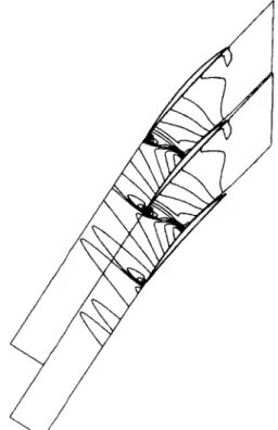
One of the goals of this work is to develop capability for analysis and design of cas-cades with intermediate blades, or splitter vanes, that are added to the basic blading to increase turning or reduce flow separation and loss. The case used as a guide for this development was a high turning supersonic compressor stage with splitter vane devel-oped and tested by the Aerospace Research Lab (ARL) in the early to mid 1970's. The high inlet Mach number and strong sidewall contraction (2:1) made this an extremely challenging test case. The blade cross-sections for the ARL two-dimensional cascade are shown in Figure 1.1. The splitter vane for this case was intended to operate in the subsonic portion of the passage downstream of the shock. The basic effect of the splitter vane on blade loading is shown in Figure 1.2, where the main blade loading is relieved

by the overlapping vane.

The ARL cascade has been the subject of several previous studies, both experimental and analytical. This cascade started out as part of a high pressure-ratio, high diffusion axial rotor developed for the USAF. Tests had indicated excessive deviation angles that were reduced by the addition of a partial flow splitter. The two-dimensional cascade was tested by Holtman et al as a single blade [2] and later with a splitter vane [3). A rotor using this concept was later designed and tested by Wennerstrom and Frost

[4],

encountering test problems from stator choking. A later experimental study [5] in 1977 examined optimization of splitter vane location.

(24)

0.0

Figure 1.1: Blade sections for ARL cascade with splitter vane.

examined the ARL cascade with and without the splitter vane, attempting to do a design study with

limited

success. A second effort

[7]

in 1978, again by Dodge, brought a much more capable inviscid 3D potential method to bear on the ARL cascade and rotor, although the

lack

of viscous blockage effects made comparisons to test data somewhat inconclusive.

The large loss levels and deviation angles from the experiment indicate that the ARL cascade has extensive separated flow, which is likely the source of problems in earlier analytical work. The current method, with its full inviscid/viscous coupling scheme, is capable of modeling these blockage effects and should give a more complete picture of the splitter vane interaction with the main blade.

(25)

C,

0.0 0.5 1.0 RRL CASCADE MACH a 1.460 P2/Pt - 1.930 AVOR - 2.242 RL CASCADE

RL CASCADE WITH SPLITTER VANE

/ I / / I' / I \ / ~Sp1itter vane * )I*% \~*-~ / II, *--~1 '~~~~~'1 / /

Figure 1.2: Effect of splitter vane on pressure distributions for ARL cascade.

1.3 Overview of Thesis

The thesis is structured so the introductory material briefly discusses the development of the method, while the bulky derivations and detailed material is presented in the appendices. A brief sketch of the contents of the thesis is given below:

Chapter 2 introduces the coordinate systems, governing equations and boundary con-ditions appropriate to the quasi-3D blade to blade problem.

Chapter 3 presents the discrete form for the equations and boundary conditions on the intrinsic streamline grid. The Newton-Raphson method used to solve the non-linear system is discussed. Design options and the modifications for multiple blade analysis and design are introduced. The offset-periodic grid and solver used for supersonic cascades is discussed.

-0.5 MISES IV 1.0

(26)

Chapter 4 exercises the method on several analysis test cases at subsonic, transonic and supersonic inlet Mach numbers to validate the quasi-3D capabilities. Solutions for the supersonic ARL cascade with splitter vane are compared to test data.

Chapter 5 examines the ARL cascade with splitter vane in greater detail. The effects the splitter vane position are analyzed and compared to test data. The splitter and main blade are redesigned to optimize loss and turning. Additional avenues for cascade modification are explored using the method.

Appendix A presents the derivation of the discrete form of the quasi-3D Euler equa-tions on the streamline grid.

Appendix B outlines the modifications to the integral boundary layer method to in-clude quasi-3D effects.

Appendix C presents the loss model and the loss sensitivity calculation used in design optimization.

(27)

Chapter 2 Theory

2.1 Cascade Coordinate Systems

The geometric quantities defining a two-dimensional cascade are illustrated in Fig-ure 2.1. The cascade blades are periodic in y with pitch yp,-ii/,. The blade chordlines

Yp

Figure 2.1: Cascade coordinate system

are inclined to x direction by the stagger angle . The inlet flow direction is f31 and the

outlet flow angle is

f2-The three-dimensional flow in an axial stator or rotor is treated as an axisymmetric meridional flow and a quasi-3D blade-to-blade flow defined on the axisymmetric stream surfaces, as shown in Figure 2.2. In this figure blade elements for the blade-to-blade flow

(28)

are shown defined by a stream surface of revolution. The axisymmetric stream surfaces are defined in terms of the radius r(z) and streamtube thickness b(z), where z is the axial coordinate, and are shown as streamlines in the meridional plane in Figure 2.3. Meridional streamlines can be determined using a through-flow method to solve the

Stream surface of revolution viewed along blade axis.

Figure 2.2: Blade-to-blade flow on a stream surface of revolution

casing

r

b

hub

z

Figure 2.3: Meridional (r-z) plane for defining stream surfaces

axial and radial equilibrium relations for mass, momentum and energy given the basic stage inflow and outflow parameters and the hub and tip casing shapes. The flow over a complete blade can be approximated by a set of quasi-3D blade-to-blade problems for stream surfaces at several radial stations, a technique that forms the basis of many preliminary design systems for compressor design.

(29)

The cascade definitions in Figure 2.1 are also used for axial stator blades with x and y corresponding to the axial coordinate z and circumferential coordinate 0. Alternatively, x and y will correspond to a local m', 0 coordinate system defined on the stream surface. This choice is advantageous because it is a conformal mapping of the surface of revolution to a plane, preserving angles and shapes. The new coordinate

m'

is defined as the normalized arc-length in the r - z plane.

, J m f (dr)_T 2 +(dz)2

(2.1)

In the current method the quasi-3D blade-to-blade flow is solved on a stream surface in an m', 0 coordinate system with specified radius and stream tube thickness.

These definitions also apply for a rotor, except that the flow problem is defined in a blade-relative coordinate system rotating with respect to an inertial frame. Referring to Figure 2.1, the blades on an axial rotor are defined to rotate with angular velocity Q in the -y direction.

2.2 Viscous/Inviscid Flow Solution

Unlike most airfoil flows, cascade flows normally exhibit strong coupling between the inviscid flow and the viscous boundary layers, particularly at transonic and supersonic Mach numbers. This coupling can be sufficiently strong, involving extensive flow separa-tion, that the flow cannot be solved without considering viscous effects on blockage, e.g. the ARL cascade in Chapter 4. Viscous effects must also be included for the prediction of cascade losses.

Instead of solving the viscous flow directly, the zonal approach of ISES is used. An equivalent inviscid flow, EIF [8], is postulated using a displacement surface to represent the viscous layer, as illustrated in Figure 2.4. The inner boundary of the EIF is displaced outward from the wall by the boundary layer displacement thickness *. The outer inviscid flow is solved using the steady state Euler equations while the boundary layer flow is solved using an integral boundary layer method. The outer flow is coupled

(30)

EIF 6- u

Figure 2.4: Equivalent inviscid flow defined by BL displacement thickness

to the boundary layer through the edge velocity and density that drive the integral boundary layer solution for the displacement thickness. These two interdependent flow domains are fully coupled by a simultaneous Newton-Raphson solution procedure for the non-linear equations.

2.3 Steady-State Euler Equations

The inviscid flow is solved using the steady-state Euler equations in a blade-relative coordinate system. The integral form for the Euler equations is derived using the conservation laws for mass, momentum and energy applied to a control volume V with boundary aV and unit normal ft.

Mass p(q - n) dA = 0 (2.2)

DV

Energy p(q -

n)

I dA = 0 (2.4)

These equations apply to a reference frame rotating with angular velocity 11 with respect to the inertial frame, adding rotational terms to the momentum and energy equations.

(31)

The source term in the momentum equation, f represents the Coriolis and centrifugal force terms in the blade relative system.

f = 0 x (fl x ie) + 21 X q (2.5)

The conserved quantity in energy equation is the rothalpy,

I,

which is invariant in the rotating system.

I = h + _(2.6)

2 2

The inviscid formulation is completed with the assumption of the ideal gas law.

h p

7 P with =c,/cc (2.7)

f - 1 p

The strategy for solving the inviscid equations is to discretize them on a streamline grid, eliminating convection terms across the streamline faces. This leads to a particu-larly simple form for the Euler equations, where the continuity and energy equations are replaced by statements of constant mass flow and rothalpy in each streamtube, leaving only the equations for streamwise and normal momentum to be solved.

2.4 Boundary Layer Solution

The viscous flow is solved using the integral boundary layer method from ISES

[91,

modified to include quasi-3D effects, see Appendix B. This is a two-equation method employing the venerable von Kirman integral momentum equation and the kinetic energy shape parameter equation. In turbulent flow regions a dissipation lag equation, similar to Green's lag equation [10], is added to model upstream history effects on the Reynolds stress. These equations have the form

-- = Ft(O,6*,u) (2.8) d [H*(0, 6*, u)] * d = .F2(,6*,ue, C-) (2.9) dC~ d = a , u , , ) (2.10) ds

(32)

Relations derived using Swafford's turbulent flow profiles provide turbulent closure for the shape factors, skin friction and dissipation.

In laminar flow regions the same basic scheme is used, with the dissipation lag equation (2.10) replaced by a transition equation. An envelope method for maximum disturbance amplification is used, based on spatial amplification of Tollmein-Schlichting waves in the Orr-Sommerfeld equation. The maximum disturbance amplitude variable N replaces C, in the BL equation set. The amplification equation has the form

dN

F4(0, 6* Uc) _(2.11)

ds

The transition point is determined by the variable N exceeding a specified critical value N... The result is roughly equivalent to the classical 0 transition prediction method. The laminar flow equations are completed using closure relations derived from correlations with Falkner-Skan profiles.

The boundary layer solution is influenced by the edge velocity u,,, which is also the surface velocity in the EIF. Correspondingly, the displacement thickness from the boundary layer influences the inviscid flow by offsetting the edge of the inviscid region from the surface. Because the inviscid and viscous solutions are fully coupled in the Newton system, flows involving separation may be calculated.

2.5 Boundary Conditions

The principal requirement for the boundary conditions is that they must completely specify the flow problem and be physically realizable. This is a more serious problem for cascades than for airfoils due to the finite domain and transonic or supersonic con-ditions into or within the passage, presenting far more opportunities to specify ill-posed boundary conditions.

The boundary conditions must specify the inflow thermodynamic quantities - stag-nation density and stagstag-nation enthalpy. Inflow direction must also be specified, although

(33)

1.0 0.8-rh/poao A 0.6 -o.4 -0.0 0.00 0.25 0.50 0.75 1.00 Mach number 1.25 1.50 1.75 2.00

Figure 2.5: Variation of mass flow with Mach number

the form this takes depends on the Mach number. One additional quantity must be spec-ified, either the mass flow or the exit pressure. Additional boundary conditions that constrain added variables (or DOF's) are required on a one-to-one basis. These are often used to drive the system to a specified flow condition or for design applications.

Some combinations of boundary conditions are ill-posed - consider the mass flow in a passage of area A, shown as a function of Mach number in Figure 2.5. Up to the point at which the passage chokes, the specification of mass flow is well-posed. Beyond the choke point, further increases of mass flow are ill-posed. In fact, the discrete equations with specified mass flow become increasingly ill-conditioned as the choking point is approached, leading to numerical problems. These can be alleviated by specifying exit pressure and allowing the mass flow be determined by the solution, which is well-posed because mass flow is uniquely specified by exit pressure, while the reverse is not true.

The Newton method used to solve the non-linear equations requires an initial flow condition from which to begin iterating to a solution. For a given mass flow in Figure 2.5 there exists two possible Mach numbers, one subsonic and one supersonic. It is essential

(34)

that the initial state correspond to the desired branch.

2.5.1 Subsonic BC's

For subsonic inflow the boundary conditions that must be specified depend on whether the flow in the passage is choked. These take the form

inflow BC outflow BC determined

Subsonic BC po, h, rn,#1 PCX*(

or

PL , ho,

T

Perin

Either of these combinations may be used for unchoked flow. Exit pressure need not be specified since pexia is uniquely determined for unchoked flow by the inlet conditions and cascade geometry. Alternatively, Pe.'i, can be specified, provided one of the inflow boundary conditions is dropped to avoid over-specifying the problem. The inlet flow angle 01 must be specified, although it should be imposed sufficiently far forward of the cascade that this specification is relatively unaffected by its flow disturbance. The inlet mass flow specifies the inlet Mach number, given the other inlet quantities.

As the flow becomes choked there is no longer a unique exit pressure for a given set of inflow conditions. The second boundary condition must be used, with peri, specified and one of the inflow boundary conditions dropped, usually mass flow since it is always uniquely determined by exit pressure.

2.5.2 Supersonic BC's

As a result of the high stagger angles used on supersonic cascades the inflow is normally also axially subsonic, i.e. MI cos 01 < 1.0. The incoming flow is influenced by the

fixed pattern of expansion and/or compression waves that run axially forward from the supersonic upper surface of the blade, see Figure 2.6. These waves turn the incoming

(35)

inlet

boundary-.

_/

LE.

waves

Figure 2.6: Supersonic/axially-subsonic inflow for cascade, showing inlet wave system

flow to approximately align with the supersonic portion of the blade upper surface. At the point where the cascade is choked the upstream flow into the infinite cascade is at the so-called "unique incidence" condition for the cascade. In practice, whenever the inflow is supersonic the range of inlet flow angles into the cascade is quite close to the unique incidence point.

Supersonic, axially subsonic BC inflow BC outflow BC determined

po, ho, Cin Pexzi

7n

The inflow angle cannot be arbitrarily specified for supersonic flow due to the in-fluence of the cascade wave system. The correct inlet condition for supersonic/axially-subsonic inflow is to specify an inlet characteristic condition so that the inlet boundary acts as a free boundary to expansion or compression waves in the flow domain, see [11, page 291]. This inflow condition is defined by

(36)

where 0 is the local inlet flow angle and v(M) is the Prandtl-Meyer function, _-_

7-1

v

= arctan

(Al

2 _-1) - arctan A/M2 _{- 1} 7+1 7+1 (2.13)

With inlet characteristic conditions the inflow angle and Mach number are no longer independent. As the inflow angle is changed by expansion or compression waves from the cascade, the local Mach number changes along the inlet characteristic. The Mach and local flow angle dependence for a family of characteristics is shown in Figure 2.7. Since the slope dO/dM vanishes at the sonic point, the Mach number becomes very sensitive to flow angle changes near M = 1.0.

0.6-0.4 -0 (radians) 0.2 - 0.0--0.2 -0.4 1- 1.1 1.2 1.3 1.4 Mach 1.5 1.6 1.7 1.8

Figure 2.7: Characteristic families for local angle 0 and Mach

2.5.3 Periodic BC

Periodic conditions for geometric continuity must be imposed on the stagnation stream-lines upstream and downstream of the blade. In addition the streamstream-lines must be force-free, set by imposing equal pressures across the periodic boundary.

-0

cig=0.4

cig=0.2

(37)

2.5.4 Solid Wall BC

Since a streamline-based solution technique is used for the inviscid flow, solid wall conditions are easily imposed since no mass flow crosses the blade surface streamline,

by definition. The solid wall boundary condition fixes the streamline position to the

blade surface, i.e. 8n = 0, where n is the coordinate normal to the surface streamline.

For viscous cases, where the EIF is displaced by the boundary layer, this becomes

Sn

= 6 (*), where

S

is the displacement thickness from the BL solution.

2.5.5 Design BC

One of the useful options for design applications is a form of inverse boundary condition where, instead of specifying the surface position and having the pressure set by the flow field, the surface pressure is specified directly and the streamline geometry is determined

by the flow solution. This is easily done within the framework of the streamline solver by imposing a wall pressure condition in place of the solid wall condition. An arbitrary

specified pressure distribution may not give a physically realizable blade, so specified pressure distributions are subject to several compatibility conditions, as discussed in

[9].

Inverse design boundary conditions cannot be applied over a separated region be-cause there exists only a very weak local constraint for surface displacement in the separated BL. A modal design scheme has been implemented, using a set of geometric shape functions (or bump functions), to circumvent this limitation. Modal design is discussed in greater detail in Chapter 3. Camber changes to achieve a specified pres-sure loading for fixed thickness may also be determined using a variant of the periodic boundary condition.

(38)

2.6 Loss Calculation

Losses through a cascade result from the entropy rise from inlet to outlet produced by inviscid shock losses and viscous dissipation in the blade boundary layers. The increase in entropy causes a reduction of the stagnation pressure from the equivalent isentropic value. The loss coefficient w is defined as the reduction in exit stagnation pressure non-dimensionalized by the inlet dynamic pressure.

- P(,,

(2.14)

Po, - PI

where

P.2

is the mass-averaged exit stagnation pressure and po, is the isentropic (i.e. lossless) stagnation pressure at the exit. Two approaches are used for calculating loss - a mass-averaged stagnation pressure defect at the exit plane, and an extrapolation to a fully mixed condition. Further details on the loss calculation are presented in Appendix C.

2.7 Non-Dimensionalization and Reference Quantities

Although the basic equations can be used with quantities having any consistent set of units, it is advantageous to impose a systematic non- dimensionalization of the quantities defining the geometry and flow. The physical quantities, such as i, etc., are

non-dimensionalized using reference quantities

2, ju

and &O.

z = . y= -Caxaal Caxial (2.15) P q P q pO ao

This means that, in the non-dimensional variables, inlet reference values for flow vari-ables are defined at r = 0 as

1 Pur 1 Pore-(2.16) 1 au,.f = 1 I= 7 -1

(39)

Chapter 3 Numerical Formulation

This chapter describes the numerical implementation of the Newton system and bound-ary conditions for the streamtube-based Euler solution with integral boundbound-ary layers.

A design capability for viscous cascade redesign using a set of geometric perturbation

modes is introduced. The basic scheme is generalized to treat multiple blade cascades and several new modes for the design of splitter vanes are introduced. Problems with regular topology grids for supersonic cascades are discussed along with the formula-tion for the new offset-periodic grid topology. Addiformula-tional details on the derivaformula-tion and implementation are presented in the Appendices.

3.1 Overview of Numerical Scheme

The viscous cascade flow is solved using a zonal approach, dividing the flow into an inviscid outer flow modeled using the steady-state Euler equations, and viscous layers over blades and in wakes modeled with an integral boundary layer method. The two zones are interacted by driving the boundary layer with the edge flow quantities from the inviscid flow, whose edge is defined by the boundary layer displacement thickness. The non-linear equations for the two zones are solved simultaneously using a Newton-Raphson solver making it possible to treat fully separated flows. The Newton solver uses a direct solution of the linearized system, making the method robust, and allowing additional well-conditioned degrees-of-freedom (DOF's) and constraint equations to be freely added to apply useful boundary conditions or design functions.

(40)

3.1.1 Inviscid Flow

The inviscid flow is solved with a conservative formulation of the steady-state Euler equations in the blade-relative coordinate system. The equations for mass, momentum and energy are solved on an I x J streamline grid of nodes that define the problem

domain, see Figure 3.1. The grid is defined by families of streamlines and quasi-normal lines indexed by j by i, respectively.

2

1 LE

Figure 3.1: Streamline grid system for discrete Euler equations.

The discrete form of the equations is derived by applying the integral equations 2.2 through 2.4 to the basic conservation cell ati, j, deufned on a streamtube between three quasi-normal lines, as shown in Figure 3.2. The use of the streamline grid considerably

jr x y r b conservation cell streamline quask-normal lin e p p q x _{y r b} Flow Variables

Figure 3.2: Conservation cell and variable locations.

5Fn

6e

(41)

simplifies the discrete form of the equations because it eliminates convection terms across the streamline grid faces. The velocity and density need only be defined on the two quasi-normal faces of the cell. Pressures are defined on quasi-normal faces as p, and on streamwise faces as IIt. The mass equation reduces to an implicit statement of constant mass flow in each streamtube.

rh l ₂ *..fl

Similarly the energy equation becomes an statement of constant rothalpy

I1 = I2 = -. = It

The two equations remaining explicitly are the components of momentum. The momen-tum forces are resolved into a streamwise, or S-momenmomen-tum, equation and a quasi-normal, or N-momentum, equation.

S. Fi~. = FSj (p, p, q, x, y, r,b) = 0 (3.1)

N = .Fv, (pp,q,II-,II+,xy,r,b) 0 (3.2)

where the forces consist of pressure, mass flux and rotational forces. Rather than use the N-momentum equation directly, the H streamline pressure variables are eliminated

by differencing the N-momentum equations on adjacent streamtubes. The resulting equation, the reduced N-momentum equation, gives the net force across the streamline directly.

F (pp, q, , y, r, b) 1 = 0 (3.3)

where the dependence is now on the variables in two streamtubes

j

and

j

+ 1. Note

that the solution of the Euler equations must result in the balancing of the streamwise forces in each streamtube and the normal forces across each streamline.

One of the advantages of this formulation is that the streamline equations require no added dissipation for subsonic flow. Dissipation is added in supersonic regions in the form of an upwinded velocity term, similar to a bulk viscosity. This term becomes significant in strong velocity gradients and stabilizes the scheme for capturing shocks. The first-order dissipation scheme from reference [9] is normally used, although a second-order dissipation scheme has been added that reduces spurious dissipation loss. Stability

(42)

problems at supersonic Mach numbers have limited the use of the second-order scheme to subsonic and transonic flows.

Corresponding to the two momentum equations for each conservation cell there must be two unknowns. These have been chosen as the changes in density

6p

on each quasi-normal cell face, and the quasi-normal displacement 6n of each streamline node, as shown in Figure 3.2. The grid node positions are therefore determined as part of the solution, making it simple to extend the basic method to design problems where the streamline shape corresponding to a specified pressure distribution is determined. The discrete form for the interior equations is fully derived in Appendix A.

3.1.2 Boundary Conditions

The system of interior equations must be closed by applying boundary conditions at the edges of the domain, see Figure 3.3 These take the form of periodic and solid wall

~~~~f

lo:6Tx0

slo _(Kutta)

All:. 0

Figure 3.3: Boundary conditions on domain boundaries.

boundary conditions on the

j

= 1 and

j

= J faces of the domain and inlet and exit slope conditions on the i = 1 and i = I faces. Although they are not unknowns in the equations, quantities for rothalpy and mass flow are also implicitly or explicitly set at

i = 1. Each streamtube also has a specified stagnation density condition set at the inlet.

(43)

The discrete form for the edge boundary conditions is summarized in Table 3.1. Pe-riodic conditions are applied across stagnation streamlines upstream and downstream of the blade, specifying Ani, the gap between streamlines

j

= 1 and

j

= J, accounting for

the pitch offset. Solid wall conditions are applied on each of the stagnation streamlines between the blade leading and trailing edge by imposing An, the gap between stream-line and the wall. These definitions for An are modified for viscous flows to account for blade and wake boundary layer displacement thickness.

Table 3.1: Discrete boundary conditions on domain edges.

The inlet flow direction is imposed by requiring that all streamline segments at i = 1 have a specified slope si-, = tan f1. For supersonic inlet conditions the inlet slope condition is replaced by an inlet characteristic condition specifying the local angle for streamlines 1 <

j

< J - 1. The angle for the remaining

j

= J streamline is set by

geometric periodicity.

Boundary type Discrete boundary condition

Anij = 0 solid surface Ani =

0

An1 = 0 periodic 0 IY2~₁- Ij = 8 n subsonic inflow X2.j - Z pl "- po = 0

supersonic inflow arcan I '(Mij) =cil

poi - Pu ₁ = 0

outflow '

Y-1,j Sout

(44)

The outlet flow direction is treated analogously to the inlet direction, and is imposed

by requiring that all segments at i = I have slope s0,₁j = tan32. In practice, to avoid

a large pressure jump at the blade trailing edge, the exit angle should be treated as an additional unknown which is set by the trailing edge Kutta condition.

The inlet stagnation density condition is imposed using

(h(2< ₎₂

(ho

-q-rgi (Or)

S ) Pore = 0 where ho = I - 2 + 2 (3.4)

The streamtube approach encourages several of the boundary conditions to be applied implicitly, written directly into the momentum equations. The rothalpy is constant in the domain and is not treated as an unknown. The mass flow is also constant for each streamtube and is treated implicitly. Mass flow is set by inflow Mach number and streamtube area at the inlet. The implicit treatment of mass flow requires special treatment for choked flow, where the mass flow is effectively determined by an imposed exit pressure. The details of the choked flow solution are discussed in Appendix D.

3.1.3 Newton-Raphson Solution

The complete set of flow equations and boundary conditions specify a large non-linear system which is solved using a full Newton-Raphson method. An initial streamline grid, roughly corresponding to an incompressible flow solution, is generated about the blades using an elliptic grid generator and supplies the initial guess for the Newton iteration. The flow field is initialized with a uniform density for subsonic flow, or a smooth gradient of density to a specified exit condition at supersonic or choked conditions.

The basic Newton method solves the general non-linear system

R(Q) = 0 (3.5)

where

Q

is the vector of variables and R is the vector of equations. At iteration level

m, the Newton solution procedure is

OR] = R"'

(3.6)

(45)

Q"f+I

=

Qm

+ 6Qrn

_(3.7)

Care must be taken with the last step when updating the variables to limit changes to ensure that the variables remain within reasonable limits. The Newton changes are clamped so that density and velocity may only change by 30% per iteration.

For the inviscid flow R consists of the S-momentum equations on each streamtube and the N-momentum equations on each streamline plus the boundary conditions at the domain edges. The vector of unknowns

Q

is made up of unknowns for the interior equations consisting of perturbations to the streamtube cell density

6p

defined on quasi-normal faces and perturbations to the streamline quasi-normal node displacement Sn. A few

additional global unknowns are normally introduced to control boundary conditions such as inlet or exit angle. One additional global constraint equation must be added to the system for each global unknown.

The Jacobian matrix

[)q

must be generated and inverted for each Newton step. This system represents the linearized change in the residual with respect to the un-knowns and is constructed by taking variations of the equations with respect to each of flow and geometric variables. These variations are resolved by repeated application of the chain rule for partial derivatives to be minimally expressed only in terms of the Newton system unknowns

6p

and Sn. For example, taking the S-momentum equation

3.1 at i, j

_Fs __s

O.Fs

0-Es

OFs

__s __s

6FS. 6P+ 8S6P+ Sq+ S+ Sy+ s6+ S6b

-p

ap

61q 19X

ay

Or

Ob

The variations bp, 6q, etc. are resolved in terms of their dependencies on 6p and Sn

using repeated applications of the chain rule, as an example the pressure variation

p(p, q, !, y, r, b) is resolved using

6 p +p /q 9r ax +p (q ax +q Oy +q ar ax

)p

6P+

+ap

+

ra

6n+--ap aq ap ar ax n aq ax an ay an

B~

where the intermediate derivatives such as a are generated and stored at each iteration level. Although it looks awkward on paper, the chain rule process is reasonably efficient at the Fortran level, at least.

(46)

3.1.4 Matrix System

The Jacobian matrix is a large linear system of I x (2J - 1) equations, made up of

(I - 2) x (J - 1) S-momentum equations and (I - 2) x (J - 2) reduced N-momentum equations. Boundary conditions supply equations on the j = 1 and j = J streamlines

and the i = 1 and i = I quasi-normal lines.

The domain of dependence for the S and N-momentum equations is relatively com-pact, as shown in Figure 3.4. The basic equations span three streamwise nodes,

corre-Vj

_Z'

A

_AC. v₁

~1 ~

,1c -M* i .1 reduced N-mom. .1. ,- ' 2. 1.1

Figure 3.4: Domain of dependence for S-momentum and N-momentum equations.

sponding to blocks Bi, Ai and Ci. The S-momentum equation spans one streamtube (two streamlines) and the N-momentum equation spans two streamtubes (three streamlines). Additional upstream dependence, due to artificial dissipation, increases the domain of dependence to include one or two additional streamwise nodes. The small 'molecule' of dependence results in a sparse Jacobian matrix whose equations are most efficiently

(47)

arranged as I block rows of (2J-1) equations in each block and have the form Ai, , I I-B2 A2 C₂ _IH2 62 -R2 Z B Bj A1 CQ 113 63 V4

j Z.I

B.4 A4 C4 I H R vi Zi B i A i _Ci _I_Hi _X _i _~~i (38 Y Z B A H 6 -( V Z B A Ci H -R Y I Z B I A, I HI I -RI G, G2 03j GGI 9 6 g R-g

The unknown vector for each block is Si (5ni,7,j, 8pii-J-i), corresponding to the

density changes and displacements on the i quasi-normal line. The Ri terms are the Newton residuals for the S-mom. and N-mom. equations. Additional global unknowns 6. _{and constraint equations, made up of Gi entries for the interior flow unknowns,} and G. entries for the global unknowns, do not fit within the compact block structure. The Hi blocks represent the effect of the global unknowns on the S-mom. and N-mom. equations. Further details on the block structure of the matrix and solution are presented in Appendix D.

3.1.5 Global Variables and DOF's

The large, sparse matrix in 3.8 is solved using a specialized direct solver that divides the full matrix into a banded matrix and a small matrix for the global unknowns. The global influence columns H are simply treated as additional right-hand sides, so that the addition of global unknowns, or DOF's to the system, increases the solution cost

by a negligible 3% per DOF. This treatment of global variables as separate unknowns

with global constraint equations adds considerable flexibility in the implementation of boundary conditions or design conditions. The equation added to constrain a DOF need only be well-posed, it does not even need to directly involve the global variable.

Analysis and design of transonic cascades with splitter vanes

3

90803 OOL66926~ 8

ANALYSIS AND DESIGN OF TRANSONIC

CASCADES WITH SPLITTER VANES

by

H.H. Youngren

GTL Report #203

March 1991

ANALYSIS AND DESIGN OF TRANSONIC

CASCADES WITH SPLITTER VANES

by

H.H. Youngren

GTL Report

#203

March 1991

This research was supported by the Air Force Office of Scientific Research, Grant

AFOSR-89-0373, with Captain Henry E. Helin as Program Manager and Dr. Arthur J. Wennerstrom as

Technical Monitor.

Analysis and Design of Transonic Cascades

with Splitter Vanes

Harold Hayes Youngren

Acknowledgements

Contents

List of Figures

List of Tables

C.1

Nomenclature

P,

j

j

A,

()

( )

(^)

(

( )o

( )

(

(

):3

(

(

);,

( ),,,,

(

isentropic

(

(

(

(

Chapter 1

Introduction

1.1

Motivation and Background

1.2

Cascades with Splitter Vanes

[4],

limited

[7]

lack

C,

1.3

Overview of Thesis

Chapter 2

Theory

2.1

Cascade Coordinate Systems

Yp

casing

r

b

hub

z

m'

2.2

Viscous/Inviscid Flow Solution

2.3

Steady-State Euler Equations

n)

_/

_Z'