Lidar observation of gravity and tidal waves in the stratosphere and mesosphere

HAL Id: insu-03117564

https://hal-insu.archives-ouvertes.fr/insu-03117564

Submitted on 2 Mar 2021

HAL is a multi-disciplinary open access

archive for the deposit and dissemination of

sci-entific research documents, whether they are

pub-lished or not. The documents may come from

teaching and research institutions in France or

abroad, or from public or private research centers.

L’archive ouverte pluridisciplinaire HAL, est

destinée au dépôt et à la diffusion de documents

scientifiques de niveau recherche, publiés ou non,

émanant des établissements d’enseignement et de

recherche français ou étrangers, des laboratoires

publics ou privés.

Lidar observation of gravity and tidal waves in the

stratosphere and mesosphere

Marie-Lise Chanin, Alain Hauchecorne

To cite this version:

Marie-Lise Chanin, Alain Hauchecorne. Lidar observation of gravity and tidal waves in the

strato-sphere and mesostrato-sphere. Journal of Geophysical Research. Oceans, Wiley-Blackwell, 1981, 86 (C10),

pp.9715-9721. �10.1029/JC086iC10p09715�. �insu-03117564�

JOURNAL OF GEOPHYSICAL RESEARCH, VOL. 86, NO. CI0, PAGES 9715-9721, OCTOBER 20, 1981

Lidar Observation

Of Gravity And Tidal Waves In The Stratosphere

And

Mesosphere

MARIE-LISE CHANIN AND ALAIN HAUCHECORNE Service d'•4bronomie du CNRS, 91370 l/erribres-le-Buisson, France

Lidar measurements of atmospheric density and temperature in the altitude range 30-to 80 km have been performed during the last 2 years from the Observatory of Haute-Provence (latitude 44øN, longi- tude, 6øE). The potential of this technique for studying the middle atmospheric structure is presented and preliminary results on wave propagation are discussed. It is shown that wave-like structures are ob- served systematically in this height range. Fourier analysis indicates that most of the energy is trans- ported by waves of vertical wavelengths on the order of 8 to 15 km. The amplitude of the density varia- tions is shown to follow a p-•/2 law up to 70 km. The characteristics of the observed density waves suggest that they are caused by a superposition of internal gravity waves propagating upward from the troposphere and a diurnal tide component in the range 30--50 km. Such waves are able to induce quite significant perturbations in atmospheric density and therefore temperature on an hourly basis. The Lidar technique is able to monitor those variations for the first time from a ground station operating continu-

ously.

INTRODUCTION SYSTEM DESCRIPTION

The

atmospheric

density

profiles

are

expected

to present For

an atmosphere

free

of aerosols,

the

light

backscattered

wave-like

structures

due to gravity

wave

perturbations.

Their by the atmosphere

from a laser

bean

is due to Rayleigh

scat-

characteristics

have been

calculated

by means

of perturbation tering by atmospheric

molecules,

unless

the emitted wave-

theory

[Hines,

1960]

and have been observed

by rocket length

coincides

with

a resonance

line of atmospheric

constit-

[Favre

et al., 1974;

Phillbrick

et al., 1974].

Calculation

and ex-

perimental

data are in satisfactory

agreement;

but, up to now,

only rocket data have been available

and only sporadically.

Therefore it has been difficult to follow the wave propagation

and to describe all its characteristics.

The results

presented

here by using Lidar sounding

from

the ground

can be obtained

on a continuous

basis,

offering

the

new possibility

of studying

the wave propagation

and its con-

sequences

on the temperature

and density

of the middle atmo-

sphere.

In the Lidar method,

the light from a laser pulse sent

vertically through the atmosphere

is backscattered

by mole-

be present

in the laser beam path. This technique

has been

atmospheric

parameters

above 70 kin. Kent and Keenliside

[1975]

have reported

what they interpret

as evidence

of tidal

modes

in the atmospheri

c density

between

70 and 100 kin.

been obtained between 80 and 100 km from the resonance

uents.

To optimize

the lidar system

to measure

neutral density

cross

section,

the energy per pulse of the laser, its repetition

rate, and the quantum efficiency

of the receiver at the laser

wavelength.

Rapidly evolving

laser

technology

precludes

a de-

time the optimal spectral

range appears

to lie around 500 nm.

In a first step, the atmospheric

density profiles were ob-

wavelengths

were used corresponding

to the sodium

or lith-

tion of this lidar facility has been given in earlier publications

[Megie

and Blamont,

1977;

Jegou

et al., 1980]

and is summa-

chopper

designed

for protection

of the photomultiplier

and

upward by the signal-to-noise

ratio. Most of the data have

been obtained

during nighttime

and so are all the data used in

this analysis.

The extension

to daytime is only recent and at

backscatter

from sodium

atoms

[Blamont

et al., 1972;

Kirchoff the present

time limited

to a range

of 50 kin. Recently,

since

1981]. The results presented here are obtained in the 30-80 km region and are therefore the first ones in this domain.

Over the last 2 years, density and temperature between 30

and 80 km have been measured from our Lidar stations at the

Observatory of Haute Provence in France (44øN, 6øE). As re-

ported earlier, a comparison

between

lidar and rocket data

Chanin [1980]. Since then, the quality of the data has in-

duction

of the spatial

or temporal

resolution.

We describe

this

technique

and present

preliminary

results

on wave propaga-

tion measurements.

Copyright ¸ 1981 by the American Geophysical Union. Paper number IC0682.

0148-0227/81/001 C-0682501.00

November 1979, the data have also been obtained with a new

lidar station

designed

for tropospheric

and stratospheric

mea-

ing. This station,

set

up alongside

the first one,

uses

for density

soundings

the first harmonic

of a Nd-Yag laser emitting 300

increased

by a factor of 10. In this station,

described

in Table

but, because

of the presence

of stratospheric

aerosols,

we have

only considered,

up to now, the data above 30 kin.

LIDAR MEASUREMENTS OF DENSITY AND TEMPERATURE IN THE MIDDLE ATMOSPHERE: EXPERIMENTAL LIMITS

AND ACCURACY

In a previous

article, [Hauchecorne

and Chanin,

1980] the

9716 CHANIN AND HAUCHECORNE: LIDAR OBSERVATION OF GRAVITY AND TIDAL WAVES IN THE MIDDLE ATMOSPHERE

TABLE 1. Major System Parameters for the Lidar Used for Night- time Mesospheric Studies at the Observatory of Haute Provence

(44øN, 6øE)

System I System 2 Emitter

Wavelength 589 nm 670 nm

Energy 1 J/pulse 0.8 J/pulse

Linewidth 8 pm 6 pm

Pulse width 3 #s 3,5/•s

Repetition rate 0.5-0, I Hz 1-2 Hz

Divergence 2 x 10 -3 tad 10 -3 rad

Divergence 2 x 10 -4 tad 10 -4 tad

(after collimation) Telescope diameter Telescope area Field of view (for nighttime) Bandwidth Receiver gate Receiver 0.818 m 0.515 m 2 5 x 10 -4 rad 0.4 nm 8/•s (1, 2 km)

* Method: photon counting combined with analogical recording.

tered signal has been described. It should be pointed out that, due to the lack of an absolute calibration of the atmospheric

transmission, the density profile needs to be fitted either to a theoretical model or to other experimental data. The reference used in this paper is the CIRA 1972 model that takes into ac- count the seasonal variation. The fitting of the experimental data with this model is performed between 30 and 35 kin. The

uncertainty of the density measurement is assumed to be the

statistical standard error. Up to the altitude where the sky

background becomes the' same order of magnitude than the laser backscattered echo, the error bar (shaded area on the fig- ures) represents 1 standard deviation and is given by the square root of the number of laser backscattered photons. In

the near future a reduction of the field of view of the receiver

will increase the range of the measurements. The height reso- lution for all the measurements presented here is either 0.6 or 1.2 kin, but a running average over 6 or 3 points has been per-

formed to improve the accuracy, reducing then the resolution to 3.6 km (except in one case corresponding to Figure 4, where the smoothing was done over 9.6 kin). Figures la and

DENSITY

• 7o

• 6o

40

A

z

--

3.6

Km

•

Fig. 1. Density and temperature data for the night of November 15-16, 1979, with 10 hours integration time and a vertical smoothing of the data over 3.6 kin. (a) The ratio of experimental density value to CIRA 72 model for November; (b) the experimental temperature pro- file (solid line) compared to CIRA 72 model (dotted line). The shaded area corresponds to +1 standard deviation.

2a present two samples of density profile as compared with the adequate CIRA model for November 1979 and August

1980, respectively. In winter the discrepancy with the model

TABLE

2. Major

System

Parameters

for the

Lidar

Used

for Strato- stays

within 20%,

while the summer

profile

disagrees

by more

(44øN, 6øE)

Characteristics of the System Emitter Wavelength Energy Linewidth Pulsewidth Repitition rate Divergence Receiver Telescope diameter Telescope area Field of view (to be reduced) Bandwidth Receiver gate In photon counting mode In analogical mode 532nm 300 mJ 0.1nm 15ns 10 Hz 3 x 10 -4 rad 0.6 m 0.28 m 2 5 x 10 -3 rad 4 t•s (600 m) 1 #s (150 m)

may be due to the inadequate position of the altitude of the mesopause in the CIRA model, which is known not to be very adequate for the summer situation.

As described in an earlier publication [Hauchecorne and

Chanin, 1980], the atmospheric temperature profile can be

computed from the density profile, assuming that the atmo-

sphere obeys the perfect gas law and is in hydrostatic equilib- rium. The atmospheric pressure at the upper limit of the mea- surements (90 kin) is fitted with the CIRA 72 model, and then

the temperature in absolute value can be deduced from 80 km

downward to 30 kin, even though the density measurements are only relative. The contribution of the extrapolated pres-

sure uncertainty

to the temperature

value becomes

negligible

measurements will always be 10 km lower than for the den-

sity. Two examples of temperature profiles are given in Fig- ures lb and 2b for winter and summer periods. The difference with the CIRA 72 model below the stratopause are, in both

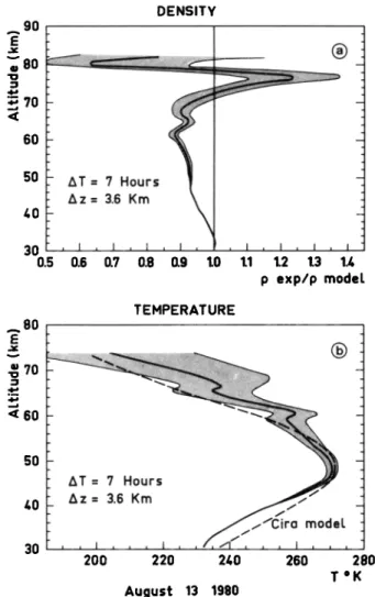
CHANIN AND HAUCIIECORNE: LIDAR OBSERVATION OF GRAVITY AND TIDAL WAVES IN THE MIDDLE ATMOSPHERE 9717 9O e 80 :• 70 6o 5o •.0 30 0.5 DENSITY _ - AT= 7 Hours - 0.6 0.? 0.8 0.9 1.0 1.1 1.2 1.3 1.t, p exp/p model. TEMPERATURE 8O

• 60

•,0

Az= 3.6 Km

_

30 '''''''''

,••,/,/C,

ir•

m,

od,,l.,

Fig. 2. As in Figure I for the •ght of August 13-14, 1980, •d a 7- hour integration period.

cases, quite large when compared to the standard deviation and are still significant above the stratopause in Figure lb.

The density and temperature profiles presented in Figure 1

were obtained with the first lidar station at the lithium reso-

nance wavelength (670 nm), while the data reported in Figure 2 were obtained with the new station at 530 rim. The accuracy in the lower part of the profiles is much improved with the

new station, owing to the gain in efficiency mentioned earlier;

but the quality of the data is still relatively poor above 60 km because of the high level of sky background that will be de- creased shortly by a factor of 100 after reduction of the field of

view.

Density and temperature accuracies with a vertical resolu-

tion of 3.6 km are presented in Figure 3 for the two experi-

mental sets of data presented in Figures 1 and 2, with 10 and 7 hours integration time, respectively. The accuracy, after the above-mentioned improvement, is also presented for 10 hours

integration time. The performances of the method for any in- tegration time T can be deduced for this figure as the accuracy will be reduced by (10/T) w2. It should be noticed that the time

resolution of the measurement is the object of a trade off with both the height resolution and the accuracy but is not likely to

be limited by the repetition

rate of the la•er (1-10 Hz). With

the performances indicated in Figure 3 the lidar technique should become a precious tool to study the thermal behavior

of the stratosphere and mesosphere with good temporal and spatial resolution.

Several objections to the use of the method have been ne-

glected in the preceding discussion. One of the most basic is

the assumption that between 30 and 80 km the atmosphere is free of aerosols, which may create a contribution to the back-

scattered signal by Mie scattering. This question can be cleared up by working with two different wavelengths, as Mie and Rayleigh scattering processes vary very differently as a

function of wavelength. Several series of measurements were

performed at two different wavelengths (670 and 530 nm) and gave simultaneous and very similar density measurements, even during the post Mount St. Helens eruption period, when

the level of stratospheric aerosols was much higher than usual.

Figure 4 presents the ratio of the two density measurements

deduced at the two wavelengths and indicates that the agree- ment is within the limits of their respective accuracy. But, a spot check at two wavelengths should be performed at regular intervals to rule out a possible contribution of meteoreric dust

or clusters at the 80 km level.

6O 5O •0 3O

-

_

////•,.

./•"'"'•

...

, ...

,

_

/i///

//

/./'

-

///•.//

-

Fig. 3. Density and temperature accuracy as a function of height for 1• -- 670 nm, AT = 10 hour (dash-dotted line); for = 530 nm, AT -- 7 hour (solid line) as expected at )• -- 530 nm and AT- 10 hours after reduction of field of view down to x 10 -4 tad. (dotted line).

9718 CHANIN AND HAUCHECORNE: LIDAR OBSERVATION OF GRAVITY AND TIDAL WAVES IN THE MIDDLE ATMOSPHERE

70

Fig. 4. Comparison

between

density

profiles

obtained

at 670 and

530 nm with an integration time of 2 hours and a vertical smoothing

over 9.6 kin.

The other limits of this method are its restriction to clear

weather conditions and to nighttime. There is little to be done about the first limit because the improvement of working at

infrared wavelengths

(10.6/an) is canceled

by a tremendous

reduction

of range. On the other hand, the restriction

of the

measurements

to nighttime can be overcome.

Our group has

recently

observed

the sodium

daytime

emission

with a signal-

sured

up to 50 km. These

daytime

measurements

are still pre-

liminary,

but they encourage

us in seeking

to obtain daytime

density

and temperature

profiles

at least up to 50 km in the

tion and diurnal variation of stratospheric temperature.

EVIDENCE OF WAVE PROPAGATION

The density

profiles

presented

in Figures

I and 2 were ob-

tively. The large difference

with the model has a tendency

to

hide the oscillating

structure

of the profile. In what follows,

to

study

the temporal

behavior

of the density

profile

the experi-

fl. Wave-like structures

appear,

then, on all the profiles

inde-

pendentiy

of the season

and for any integration

time

ranging

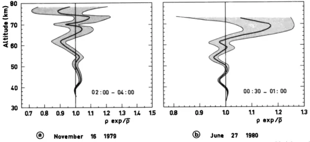
from a few minutes up to a few hours. Figure 5 presents two

examples of such profiles: the winter profile (Figure 5a) ob-

tained at 670 nm with 2 hours integration time, the summer

one (Figure 5b) at 530 nm with half an hour integration time. All of the profiles that have been recorded in the last 2 years

of measurements exhibit such a wave-like structure. The den-

sity oscillates around an average profile with amplitude reaching 5% of the ambient density at 50 km and up to 15% at

70 km. This increase in the amplitude of the perturbation with height is a characteristic feature of all our data. For most of

the altitude range up to 70 km, the amplitudes of the density variation are larger than the standard deviation and thus can

be considered as significant.

CHARACTERISTICS OF THE WAVE PROPAGATION

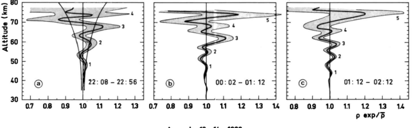
The improvement in temporal resolution of the density pro- file has been an important step forward in the study of the wave propagation. The profiles obtained recently (Figures 6a, 6b, 6c) exhibit very well-defined structures indicating clearly a downward propagation of the phase between 40 and 75 kin. From this figure we deduce a vertical wavelength of 7.5 kin. The amplitudes of the oscillations around the mean density, increasing with height as mentioned before, can be studied as a function of height. From such set of data it has been shown

(Figure 6a) that, between

40 and 70 kin, the amplitude

varies

have been able to describe some of the characteristics of the waves observed.

To present a global picture for the full periods of observa- tion and to highlight some feature of the wave propagation the density variations are presented as isopleths of per-

turbations about the mean value calculated for the whole

night. Amplitude of the variation has been corrected for the p-l/2 variation in all the following contour maps. Density in- creases, corresponding to p > rS, are represented by positive

values and are indicated on the maps by the shaded areas, while data corresponding to negative perturbations (p _< IS) are

indicated by the clear zones. Isopleths of the density per-

turbations

Ap are plotted by steps

of 2 x 10

-2 (g m-a) !/2 for

8O 7o

• •0

30

,i ....

i ...

• ....

i ....

(•) November

16 1979

•

June 2? 1980

Fig. 5. Individual

density

profiles

p normalized

to the averaged

nighttime

density

fl. (a) Obtained

with 2 hours

in-

tegration

time on November

16, 1980;

(b) with half an hour integration

time on June

27, 1980.

CHANIN AND HAUCHECORNE: LIDAR OBSERVATION OF GRAVITY AND TIDAL WAVES IN THE MIDDLE ATMOSPHERE 9719

80

.• 70

0.7 0.8 0.9 1.0 1.i 1.2 1.3 1./.

I 01'12-

02'

12

Fig. 6. Series

of three

density

profiles

normalized

to the nighttime

profile

during

the night

of August

13-14,

1980.

Waves structures are identified and indicated by numbers I to 5. Representation of the p-l/2 law on Figure 6a was calcu-

lated with Ap/p = 2% at 50 km.

the quantity Ap X •O -1/2. The data presented here correspond

to three different periods of the year, November (Figure 7),

June (Figure 8), and August (Figure 9), and do not indicate any obvious seasonal variation. It should be mentioned that

data obtained during stratospheric warmings have been delib- erately excluded because of the influence of planetary wave over powering the influence of gravity waves, and those data are presented in another article [Hauchecorne and Chanin,

1981]. A general feature in all the data is the evidence of a downward phase propagation with a phase velocity varying with height. Between 50 and 70 km a phase velocity of about 4

indicates a 3-4 hour period. From 50 km downward, the same structures are sometimes present, but, in most cases, they are

hidden by a much slower phase descent (--•0.5 km/hour), half a period during the night, indicating a 24-hour period (Fig- ures 7, 8, 9). The number of data available to build such maps

is still too limited to perform a statistical study of the wave

propagation, but the examples presented here give a first in-

dication of the variation of density, and therefore temper- ature, in the stratosphere and mesosphere on an hourly basis.

More accurate information about the vertical wavelength of the density waves have been derived from the lidar data by

km/hour associated with vertical wavelengths of about 8 km using the Fourier analysis technique in the range 30-70 km.

-• 8O

Fig. 7. Map contour of density perturbations from the mean

nighttime value for the night of November 15-16. The amplitude of the perturbation is corrected by p-l/2 and contour lines (solid) are plotted by step of 2x10 -2 (g m-3) •/2. The zero perturbation line is represented by a solid heavy line that separates the clear area (de- crease of density) from the shaded area (positive perturbations).

The analysis was performed by smoothing the extreme limits of the height range by using a Blackman window to eliminate ghosts. The analysis of 10 sets of data indicates that most of

the time two components are present in the energy spectrum,

but the larger part of the spectral energy is always found for

vertical wavelengths ranging from 8 to 15 km. The secondary

maximum corresponds either to a shorter wavelength in sum-

mer (6-8 km) or to a longer one in winter (20-27 km). As in- dicated on the two spectra of Figure 10, the relative impor-

._.70 E • 60 5O 4O

/

,I

9720 CHANIN AND HAUCHECORNE: LIDAR OBSERVATION OF GRAVITY AND TIDAL WAVES IN THE MIDDLE ATMOSPHERE

21 22 23 00 01 02 03 21 22 23 00 01 02 03 Time 6blT Time GMT

August

12

1980

I August

13

1980 August

13

1980

J

August

1/,

1980

ible with gravity waves, and the downward phase velocity in- dicates that the observed variation could be explained by a gravity wave generated in the troposphere and propagating upward. To confirm this hypothesis it is necessary to check whether the characteristics of the observed density per-

turbations can be explained by internal gravity waves.

From the series of density profiles obtained on August 13, 1980 (Figure 6), the characteristics of such a gravity wave

have been completely described and the values of the differ-

ent physical quantities related with such a wave (wind, energy flux) are in agreement with what is expected in this height range. The whole series of profiles recorded during the night

of August 13-14, 1980, from which three profiles are shown on

Figure 6 indicates a vertical wavelength of 7.5 _+ I km, a phase velocity of 2.2 _+ 0.1 km/H leading to a period of 3«

hours. It was verified on that specific example that between 40 and 60 km, the amplitude of the oscillations was constant if

corrected by p-•/2 and the average value of the product Ap x

Fig. 9. As in Figure

7 except

for the nights

of (a) August

12-13

and p-•/2 was on the order of 2 x 10

-2 (g m-3) •/2 corresponding

to

(b) August

13-14,

1980.

a variation

of 2% of the atmospheric

density

at 50 kin. The in-

tance of the energy at the two wavelengths is highly variable. In the case of August 12, 1980 (Figure 10a), two vertical wave- lengths are sharply defined at 6 and 14 kin. On June 26 (Fig-

crease of the amplitude of the density oscillation above 60 km

will be discussed later.

From those experimental data one can estimate the hori- zontal wavelength taking into account the simple relationship

between the horizontal and vertical wavelengths ()•x and

ure 10b) all the spectral

energy is found for a wavelength

of respectively)

for such a gravity wave. Assuming

a Brunt Vais-

ala period Tev of 360 s at 50 kin, the relationship 12.5 km, as it can be guessed from the vertical profile repre-

sented on Figure 5b.

Note that the frequently occurring vertical wavelengths (8-

15 kin) is identical to the wavelengths observed in the vertical

motion field in the same altitude range by Weisman and Oli- vero [1979], even though their data refer to the equatorial re- gion.

DISCUSSION

Even though the results are preliminary and the data set too

limited to allow a statistical study, it appears that two systems of waves are present in this height range: tidal and gravity

waves.

The existence of waves propagating upward with a 24-hour

period in the altitude range 30-50 km led us to think that such

waves should be from tidal origin. A theoretical calculation of the amplitude and phase of the density variations due to tidal waves was performed to check if the characteristics of the pre- dicted waves would be in agreement with the observations. The calculation was based upon the Lindzen [1967] theory in which the temperature profile was taken from the U.S. Stan- dard Atmosphere. If the 24-hour period wave observed be-

tween 30 and 50 km is to be explained by the diurnal tide, one

should expect from the theory a decrease of the density during

the night with an amplitude increasing with altitude (forced

component of the diurnal tide). Both the average density de-

crease between 35 and 45 km (•1% in 6 hours, Figure 9) and the phase (maximum of density at the beginning of the night)

are in agreement with the tidal theory. But it should be men- tioned that the normalization of the density profiles between 30 and 35 km may mask the expected density decrease and in-

dicate an artificial phase descent (Figure 8a).

Both phase and amplitude disagree with a tidal model for the 4-4 hour period waves observed above 45 kin, but, on the other hand, as it has been shown earlier, the amplitude of

those waves obey the p-•/2 law (as expected from internal

gravity waves). The range of vertical wavelengths is cornpat-

lOO E 80 August 12 1980 30- 70 krn • 40 -

ta 0 ß

eo

60

•o

_

/•

June

26 1980

(•)_

Fig. 10. Spectral energy as a function of the inverse of the vertical wavelength for (a) August 12, 1980, and (b) June 26, 1980.

CHANIN AND HAUCHECORNE.' LIDAR OBSERVATION OF GRAVITY AND TIDAL WAVES IN THE MIDDLE ATMOSPHERE 9721

• T

leads to an horizontal wavelength of 260 km. One can also es-

timate the horizontal wind velocity associated with such a

density variation. From Hines [1960], the variation of the hori- zontal wind component A v and the variation of the density Ap is given by

C Ap

/iV-- •

(7- 1) •/2 P

where C is the sound speed 330 m s -• at 50 km and 7 -- Cp/Cv is the ratio of heat capacities: 7/5 for the air.

Then it appears that a density variation of 2% corresponds to a wave-induced horizontal wind velocity of 10 m s -• value that is very reasonable at 50 km [Groves, 1980].

The the upward propagating energy flux Fz, can be calcu-

lated from the relation

1

•z

1 C

•

p-•/2)

•

Fz--- •-pA•

a -•---- 2 7-'

(Ap

X

-•

and is found to be equal to 3 x 10

-2 W m -2 value, which is

compatible

with the value of 10

-• W m -2 for the flux coming

The large amplitude of the density perturbation observed above 70 km (up to 20% of the average density) should still be

looked at with caution until the accuracy of the measurements

in that height range is improved. However, a different atmo- spheric behavior is not surprising above 70 km where the up- ward propagating internal gravity waves may degenerate into turbulence. One should also consider the possible super- position in that height range of gravity wave of thermospheric and tropospheric origins. This aspect should be investigated with data of better quality that are expected in that altitude range in a near future.

CONCLUSION

Density profiles obtained from lidar soundings have shown systematic wave-like structures. Such density perturbation are interpreted as a superposition of internal gravity waves propa-

gating

upward from the troposphere

in the altitude range 30-

70 km and diurnal tides between 30 and 50 kin. Propagation of such waves as well as their influence on the atmospheric

density and temperature can now be studied on a continuous basis by lidar soundings from the ground.

,•cknowledgments. The authors wish to thank C. Fehrenbach, Di- rector of the Haute Provence Observatory, for his hospitality. They are very grateful to all the members of the lidar team of the Service

d'A6ronomie for their contribution in collecting the data. This work

was supported by D.R.E.T. under contract 77 280 and 79 442.

REFERENCES

Blamont, J. E., M. L. Chanin, and G. M6gie, Vertical distribution and temperature profile of the nighttime atmospheric sodium layer ob- tained by laser scattering, Ann. Geophys., 28, 833-838, 1972. Favre, A. C., E. A. Murphy, and R. O. Olson, Atmospheric density

temperature and winds measured during Aladdin II, in Space Re- search XIV, p. 97, Akademie-Verlag, Berlin, 1974.

Gossard, E. E., Vertical flux of energy into the lower ionosphere from internal gravity waves generated in the troposphere, J. Geophys. Res., 67, 745, 1962.

Groves, G. V., Seasonal and diurnal vairations of middle atmosphere winds, Phil. Trans. R. Soc. London, Set. A, 296, 19-40, 1980. Hauchecorne, A., and M. L. Chanin, Density and temperature pro-

files obtained by lidar between 30 and 80 km, Geophys. Res. Left., 7, 565, 1980.

Hauchecorne, A., and M. L. Chanin, Le Lidar: Un instrument d'6tude de la temp6rature stratosph6rique at m6sosph6rique, Notes C. R. Acad Sci., Paris, 292, 1981.

Hines, C. O., Internal atmospheric gravity waves at ionospheric

heights, Can. J. Phys., 38, 144 1, 1960.

Jegou, J.P., M. L. Charfin, G. M6gie, and J. E. Blamont Lidar mea-

surements of atmospheric lithium, Geophys. Res. Lett., 7, 995-998,

1980.

Juramy, P., M. L. Chanin, G. M6gie, G. F. Toulinov, and Y. P. Dou-

doladov, Lidar sounding of the mesospheric sodium layer at high latitude, submitted to J. Atmos. Terr. Phys., 43, 209-215, 1981.

Kent, G. S., and W. Keenliside, Laser radar observations of the O3 TM

diurnal atmospheric tidal made above Kingston, Jamaica, J. Atmos.

Sci., 32, 1663-1666, 1975.

Kirchoff, V. W. J. H., and B. R. Clemesha, Atmospheric sodium

measurements at 23 ø S, J. Atmos. Terr. Phys., 35, 1493-1498, 1973.

Lindzen, R. S., Thermally driven diurnal tide in the atmosphere, Q. J.

R. Meteorol. Soc., 93, 18-42, 1973.

Lindzen, R. S., Thermally driven diurnal tide in the atmosphere, Q. J.

R. Meteorol. Soc., 93, 18-42, 1967.

M6gie, G., and J. E. Blamont, Laser sounding of atmospheric sodium: Interpretation in terms of global atmospheric parameters, Planet.

Space Sci., 25, 1093-1109, 1977.

Phillbrick, C. R., D. Golomb, S. P. Zimmerman, T. J. Keneshea, M. A. Mac Lead, R. I. Good, B. S. Dandkar, and B. W. Reinisch, The Aladdin II experiment, II, Composition, in Space Research XIV, p.

89, Akademie-Verlag, Berlin 1974.

Richter,

E. S.,

and

C.

F. Sechrist,

Jr.,

Geophys.

Res.

Left.,

6, 183,

1979.

Rowlett, J. R., G. S. Gardner, E. S. Richter, and C. F. Sechrist Jr., Li- dar observations of wavelike structure in the atmospheric sodium layer, Geophys. Res. Left., 5, 683-686, !978.

Weisman, M. L., and J. J. Olivero, Evidence for vertical motions in

the equatorial middle atmosphere, J. Atmos. Sci., 36, 2169-2182,

1979.

(Received September 30, 1981;

revised February 17, 1981; accepted April 13, 1981.)