Alfvén wings at Earth's magnetosphere under strong interplanetary magnetic fields
11
0
0
Texte intégral
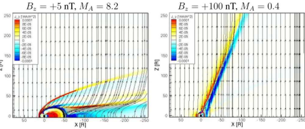
Figure

+3
Documents relatifs