by
Han Wu
B.S. Civil & Environmental Engineering University of California, Los Angeles, 2014
SUBMITTED TO THE DEPARTMENT OF CIVIL AND ENVIRONMENTAL ENGINEERING IN
PARTIAL FULFILMENT OF THE REQUIREMENT FOR THE DEGREE OF
MASTER OF ENGINEERING
IN CIVIL AND ENVIRONMENTAL ENGINEERING AT THE
MASSACHUSETTS INSTITUTE OF TECHNOLOGY
ARCWNES
MASSACHUSETTS NSTITUTE OF _fECHNOLOLGYJUL 02 2015
LIBRARIES
JUNE 20152015 Han Wu. All Rights Reserved.
The author hereby grants to MIT permission to reproduce and to distribute publicly paper and electronic copies of this theses document in whole or in part in any medium now known or hereafter created.
Signature of Author:.
Certified by:
Accep-nted hv:
Signature redacted
Department of Civil and Environmental Engineering May 21, 2015
Signature redacted__
' Pierre GhisbainLecturer of Civil and Environmental Engineering hysis Supervisor
Signature redacted
f 7leidi Nepf Donald and Martha Harleman Professor of Civil and Environmental Engineering
by
Han Wu
Submitted to the Department of Civil and Environmental Engineering on May 21, 2015 in Partial Fulfillment of the Requirements for the Degree of
Master of Engineering in the Field of High Performance Structures
Abstract
The need for economic consideration in structural design triggered the emergence of performance-based design to minimize material waste while achieving better performance. The displacement measurements of structures are significant to structural damage evaluation, and most seismic design methods consider the effect of peak ground acceleration, while the frequency content of seismic activities remains largely unexplored. In order to better understand the impact of low magnitude seismic activities on non-structural damage, we develop an assessment method for a specific site by comparing structural response with
frequency content analysis on corresponding seismic activities.
A method of analyzing frequency content of seismic activities at San Francisco is presented. By computing Discrete Fourier Transforms, time history seismic data is transformed from time
domain to frequency domain.
We apply structural response analysis on a representative residential/office/mixed-use building to evaluate seismic performance. We scale earthquakes with respect to the natural frequency of the target structure, and structural response simulations are performed based on scaled earthquakes. We utilize linear analysis in structural response simulations with constant damping ratio. The applicability of linear analysis as well as varying damping ratio requires further justification.
A comparison between frequency content analysis and structural response is presented. The
frequency content analysis provides an amplitude distribution for each seismic activity, and the magnitude of structural response is influenced by the amplitude distribution for corresponding seismic activities.
The work presented in this thesis would not have been accomplished without the support of my thesis advisor, Dr. Pierre Ghisbain. His extraordinary knowledge in structural engineering has inspired and promoted this research. I am grateful for his academic support, as well as
mentorship during my stay at MIT.
The department of Civil and Environmental Engineering at MIT provides me with a great environment to accomplish this thesis. I am grateful to all my classmates for contributing
countless new ideas on this research. Also, I am particularly grateful to Prof. Jerome Connor for his advocacy in performance based engineering, with whom discussion of this work has inspired incredible improvements.
Table of Contents
Chapter 1. Introduction ... 10
1.1 Perform ance-Based Earthquake Engineering ... 10
1.2 Frequency Content Analysis ... 11
1.3 N on-Structural D am age A ssessm ent... 12
Chapter 2. Frequency Content Analysis... 13
2.1 Introduction...13
2.1.] Site Specification...13
2.1.2 D ata Selection...15
2.1.3 Chapter Objectives and Organization... 15
2.2 Proposed M ethod ... 16
2.2.1 Procedure...16
2.2.2 Fast Fourier Transform ... 18
2.3 Seism ic Data Analysis... 20
2.3.1 Earthquakes and Records ... 20
2.3.2 Records Set Filtering...27
2.3.3 Frequency Content of Seismic Data... 30
2.4 Sum m ary...33
Chapter 3. N on-Structural Dam age A ssessm ent ... 35
Table of Contents
3. L I Sample Structure ... 35
3.1.2 Chapter Objectives and Organization ... 35
3.2 Sam ple Structure D esign ... 36
3.2.1 D esign Assumptions ... 36
3.2.2 Simplified Gravity D esign ... 37
3.3 Structural Response ... 39
3.3.1 SD OF ... 39
3.3.2 Seism ic D ata Scaling ... 40
3.3.3 Finite Element Analysis ... 43
3.4 Sum m ary ... 53
Chapter 4. Conclusions ... 55
4.1 Sum m ary of Contributions ... 55
Appendix A ... 60
Appendix B ... 71
Appendix C ... 87
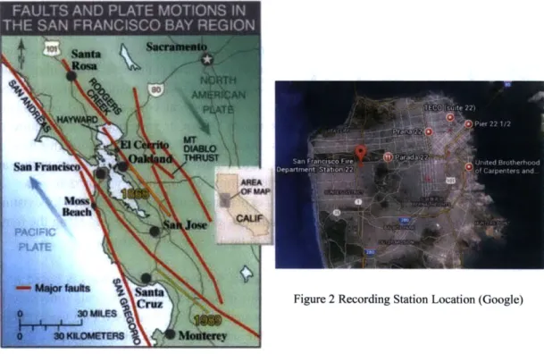
Figure 1 San Francisco Fault M ap...14
Figure 2 Recording Station Location... 14
Figure 3 NGA W EST-2 User Interface ... 17
Figure 4 NGA-W EST 2 Input Interface ... 22
Figure 5 Strike Slip Fault...24
Figure 6 Selected Time History Acceleration ... 26
Figure 7 Selected Discrete Fourier Transforms ... 31
Figure 8 Cut off Discrete Fourier Transform ... 32
Figure 9 Sample Structure First Dynamic Mode ... 40
Figure 10 RSN8617 Acceleration (top) and Displacement (bottom)... 44
Figure 11 RSN 12192 Acceleration (top) and Displacement (bottom)... 45
Figure 12 RSN 19427 Acceleration (top) and Displacement (bottom)... 46
Figure 13 RSN21418 Acceleration (top) and Displacement (bottom)... 47
Figure 14 RSN 12980 Acceleration (top) and Displacement (bottom)... 48
Figure 15 Maximum Acceleration ... 52
Figure 16 Rank Comparison ... 54
Figure 17 Maximum Displacement ... 54
Figure 18 W eight Distribution ... 57
Chapter 1. Introduction
Chapter 1. Introduction
1.1 Performance-Based Earthquake Engineering
Earthquake is one of the most catastrophic natural hazards known to human beings. The earthquake happens as a result of sudden slip between two chunks of earth lying alongside each other (Wald 2008). Due to limitations on current technology, earthquake early warning system is only capable of alarming people after an earthquake has been triggered instead of forecasting upcoming earthquakes. As most of the populated and urbanized areas are located in seismically active zones, the threat of seismic activities on built environment increases as population grows.
Building is the type of structure that provides people with sheltering but unfortunately the specific structure that is exposed to the most direct damages in seismic activities. As a result of life threatening situations, focus on quality of design and construction of structures are increasingly high. In 2008, a catastrophic earthquake with Richter magnitude of 8.0 hit China and caused tremendous casualties with 69,000 deaths and 18,000 missing (Global Risk Miyamoto, 2008). This heartbreaking event followed by two other earthquakes in Haiti and Chile in 2010 emphasize the importance of seismic analysis and design.
Despite the lack of seismic design code requirement in under-developed countries or even in developing countries, developed countries, such as United States, have established comprehensive standards regarding seismic design. However, since every earthquake is different in terms of behavioral characteristics, it is extremely difficult to compare earthquakes across different regions. Therefore, code specific seismic design tends to be over-generalized, and as a result, unnecessarily wasting economic resources.
Performance based earthquake engineering is highly appreciated under the situation of increasing seismic risk. In performance based earthquake engineering, structures are designed and analyzed through iterations. The very approach tends to provide better design in terms of utilizing economic resources and performance under seismic activities. Although design codes incorporate performance-based features, the pure performance based design process is different from code based design in terms of evaluation method.
1.2 Frequency Content Analysis
Every seismic activity can be decomposed into two major components, namely frequency and magnitude. Most seismic analysis methods that predict structural responses are focusing on magnitude of the activity. Magnitude of seismic activities is typically represented by measuring ground accelerations. As ground acceleration is the primary measure of seismic activities, the major analysis focus of seismic activities is on the response of structures with respect to ground accelerations. On the other hand, earthquake is a cyclic behavior of waves with different magnitudes, and thus the frequency of seismic activities is represented by measuring the number of cycles of wave occurring in a specified period of time (Shearer, 2010).
As mentioned in section 1.1, earthquake is a natural behavior due to sliding between two pieces of earth, and the failure surface between these two pieces of earth is called the fault. Since faults are developed after earthquakes, the probability of earthquake happening again at faults is extremely high. Therefore, seismic activities tend to be periodic with decreasing return periods as magnitude of earthquakes increases. As some urbanized areas are built on faults,
earthquake activities at these specific locations are unavoidable.
While the effect of ground accelerations on structures are drawing great attention, the effect of frequency content on structural behaviors remains largely unexplored. Also, besides avoiding resonance, design codes contain very few discussions on frequency behavior while heavily incorporating peak ground acceleration analysis. As the result of cyclic nature of seismic activities, low magnitude earthquakes tend to happen more frequently than high magnitude earthquakes. However, design codes focus primarily on high magnitude earthquakes and their effects on structural damage. The reason behind is that although most structures experience limited high magnitude earthquakes during their lifetimes, the damage due to such earthquakes is catastrophic, while low magnitude earthquakes cause no structural damage or limited structural damage.
Structures have different natural frequencies due to variations in stiffness and mass. And the natural frequency of structures affects their responses when experiencing earthquakes with different frequency contents. The frequency of earthquakes experienced by a specific structure changes with the fault type, soil condition between fault and the site and many other variables. Although comparing different earthquakes across regions is difficult, it is reasonable to compare earthquakes at the same location with similar magnitudes.
Chapter 1. Introduction
1.3 Non-Structural Damage Assessment
As structures are used for different purposes, non-structural damage begins to draw attention. The importance of non-structural damage is emphasized after the earthquake with a magnitude of 6.0 hit Napa Valley, California, in 2014. While causing no casualties, the estimated economic damage is over $400 million. Although Napa Valley is not a typical representative of non-structural damage examples due to its high storage value, the very event does demonstrate the necessity for non-structural damage considerations. (EERI, 2014)
Despite the economic impact of non-structural damages, other non-structural damages may even cause casualties. Structures with different purposes have different non-structural damage after earthquakes. According to FEMA, common types of nonstructural earthquake damages are separated into three categories, namely Life Safety, Property Loss, and Functional Loss. These categories include heavy exterior cladding, heavy interior walls, unbraced masonry parapets or other heavy building appendages, unreinforced masonry chimneys, suspended lighting, large/heavy ceilings, tall/slender/heavy furniture, heavy unanchored contents (including televisions, computers, countertop laboratory equipment and microwaves etc.), glazing, fire protection piping, hazardous materials release, gas water heaters, and other components, such as elevators (FEMA, 2012).
Chapter 2. Frequency Content Analysis
A method to evaluate the frequency content of seismic data is presented in this chapter. The
Fast Fourier Transform method is proposed for the data transformation from time space to frequency space. All data processed and analyzed are borrowed from the NGA West 2
database at the Pacific Earthquake Engineering Research center.
2.1 Introduction
This section introduces the approach to seismic data selection and transformation, as well as its corresponding methodology. This thesis is based on the data and analysis done in this chapter. Basic methodology and formulae used in this chapter are defined in this section.
2.1.1 Site Specification
As mentioned in Chapter 1, seismic activities are generated due to relative earth movement. Although most important faults are along the boundaries between continents, many other faults are located everywhere. These failure surfaces vary dramatically in terms fracture types and corresponding geotechnical characteristics. It is not practical comparing and contrasting different earthquakes across different failure surfaces. Also, the response of a structure to seismic activities is influenced by the soil conditions and geotechnical characteristics both at the structure site, and along the route of seismic wave transmission. Active faults within an area are relatively permanent comparing to the lifetime of structures within that area. A
structure locating in the active seismic zone will experience earthquakes generated by existing faults within this area. Also, geotechnical conditions at the structure site and along the route between the site and the fault will vary limitedly in the lifespan of the structure.
Based on the site oriented characteristic, the analysis performed in this thesis is based on a specific site, and the site chosen for further analysis is San Francisco. All data processed in
this thesis is recorded from the seismic station located at the San Francisco Fire Department, 22 Golden Gate Park. The specific location of the seismic station is labeled in Figure 2.
The advantages for choosing San Francisco are listed below:
M San Francisco is located in an active seismic zone. U.S. west coast is a seismic active
zone, and therefore seismic data are widely available. Figure 1 shows the seismic map of San Francisco area with all faults labeled out. Also, non-structural damage
Chapter 2. Frequency Content Analysis
is normally caused by low magnitude earthquakes like the Napa Valley Earthquake, which creates a monetary loss of $400 million.
0 San Francisco is a highly populated area. According to data in 2014, Average household income in San Francisco is $79,624, which is above national average of
$52,250. And thus seismic activities will trigger relatively high non-structural damage cost within this area and more life threatening situations. Running seismic activities analysis within this area is meaningful (Noss, 2014).
0 All data processed in this thesis is recorded by the San Francisco Fire Department
seismic station. Data recorded at the very specific site is representative of characteristics of seismic activities experienced at this site. And thus, we make an assumption that the data recorded at this site can be used to predict possible seismic activities in the future at this very site.
Figure 2 Recording Station Location (Google)
2.1.2 Data Selection
Data recorded at the recording station in the San Francisco Fire Department are borrowed from PEER center, and all data are accessed using NGA West 2. The NGA West 2 provides readily filtered time history data sets, as well as scaled response spectra. However, considering the frequency content focus of this thesis, only time history data are accessed, and the seismic data are scaled based on the ASCE 7-10 response spectrum at the natural frequency of the structure analyzed in this thesis. More details about scaling earthquakes are discussed in section 3.3. Also, detailed data selection procedures and summary of data set are discussed in section 2.3.2.
2.1.3 Chapter Objectives and Organization
This chapter discusses the implementation of Fast Fourier Transform of seismic data by converting time history data from time space to frequency space. The objectives of this chapter are: 1) Evaluating frequency content characteristics of earthquakes of the chosen site; 2) Preparing data set for later structural damage analysis. The results of the analysis in this chapter are: 1) The summary of the relationship between earthquakes and their corresponding frequency content; 2) The filtered earthquake records available for structural analysis.
This chapter first demonstrates the proposed method of transforming seismic data, Fast Fourier Transform in section 2.2. And in section 2.3, detailed data processing procedures along with analysis results are discussed. Finally, section 2.4 summarizes the findings on frequency content of earthquake records and provides summary of scaling factors for processed earthquake records.
Chapter 2. Frequency Content Analysis
2.2 Proposed Method
A commonly used procedure to transform data from time space to frequency space is presented
in this section. It is followed by an explanation of the methodology behind Fast Fourier
Transform and its corresponding implementation. Specific terminologies and functions are
presented in this section as well.
2.2.1 Procedure
The proposed frequency content analysis procedure basically includes two parts: 1) Accessing site specific seismic time history data records from NGA West 2; 2) Applying Fast Fourier Transform to process desired data. NGA West 2 is a ground motion database operated by the Pacific Earthquake Engineering Research Center (PEER). Filtering data from the database
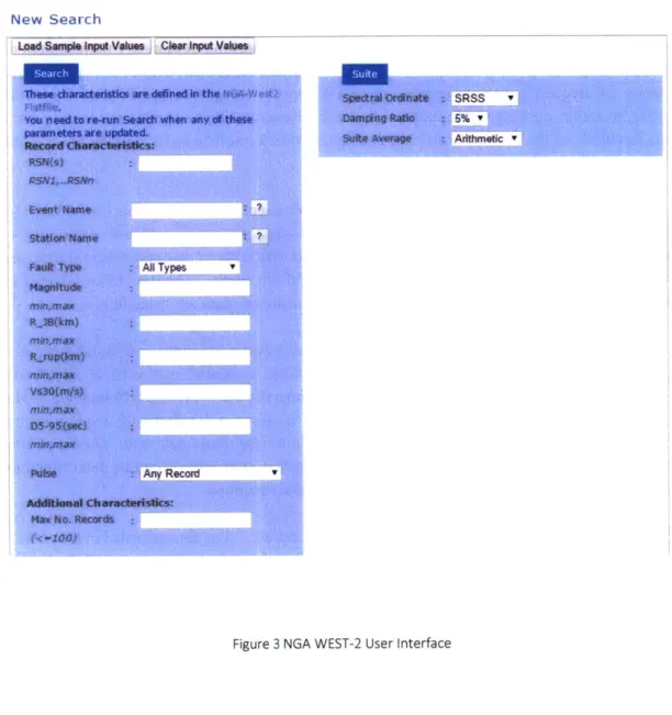
requires different input parameters. Figure 3 illustrates the user interface of the database,
illustration of input parameters are listed below:
RSN Event Name Station Name Fault type Magnitude R_JB (km) R-rup (km) Vs30 (m/s) D5-95 (sec)
record sequence number, each record in the data base is given a unique record sequence number, it can be used to locate a specific record
event name, each earthquake event is given a name, the system will search for the input string in the event name field of the database
station name, the system will search for the input string in the station name field of the database
fault type, selection for fault types including strike slip, normal/oblique, reverse/oblique, and combinations of these three fault types
magnitude of the earthquake, Richter magnitude is used in the magnitude
field
closest distance to the surface projection of the fault plane
closest distance to the surface projection of the rupture plane
time-averaged shear-wave velocity to 30-meter depth.
Pulse pulse, selection for types of earthquake including pulse like records, no pulse like records and any records
New Search
Load Supe Input Values CinpW Vakm
Chapter 2. Frequency Content Analysis
2.2.2 Fast Fourier Transform
Fast Fourier Transform is an algorithm used to compute the discrete Fourier transform. The purpose of the Fourier transform is converting a signal from a time domain to frequency domain. Discrete Fourier transform converts a finite list of functions into a list of finite combination of complex sinusoids. And these complex sinusoids are combined with coefficients accordingly to produce the same value as of the original functions. Speaking of that, any wave functions can be decomposed into a combination of sinusoidal functions, and these functions are arranged in terms of frequency and corresponding coefficients. Results of the Fourier transform include frequency content distributions of a specific wave function. The characteristics of the wave functions of the Fourier transform enable us to performe frequency content analysis on seismic records. (Heckbert, 1998)
Fast Fourier transform is an ideal method to compute Fourier transforms. This method rapidly computes coefficients or factors of a discrete Fourier transform matrix with a fixed number of sinusoidal functions, and by factorizing most of the coefficients to zero, the original function can be expressed with a product of different sinusoidal functions. The two major benefits of applying fast Fourier transform to ground motion time history data are listed below:
" Ground motion activities are represented using wave functions. Ground motion is
the simple shaking behavior of earth in both horizontal and vertical directions. However, ground motion is complex to compute since it combines different sinusoidal functions in a single event. Using Fourier transform will effectively decompose the ground motion into a combination of sinusoidal functions with corresponding coefficients, and thus frequency content of each ground motion can be determined by evaluating different combinations of sinusoidal functions.
" Each ground motion record is numerically intensive. For data recorded in NGA West 2 database, the sampling frequency is 100 Hz. For a ground motion activity lasting for 100 seconds, there are 10,000 data points recorded. Therefore, fast Fourier transform provides a rapid way of computing discrete Fourier transforms. Also, ground motion data includes a considerable amount of noise, applying fast Fourier transform can effectively determine the weight of different sinusoidal functions at different frequencies, and therefore produces a more intuitive observation of frequency content of ground motion activities.
Discrete Fourier transform is equivalent to continuous Fourier transform known only at a finite instants separated by sample times T. The Fourier transform function is expressed as follow:
F(o) = ff(t)e-aitdt (2- 1)
where W angular frequency, [rad/s]
t time, [s]
F(a) Fourier transform of original signal
f (t) original signal
The function (2- 1) illustrates the Fourier transform of a continuous signal. However, the integration of the continuous-time signal over infinite upper and lower bounds is neither practical nor necessary. For ground motion data processing, signals are processed using sampled form with a specific time interval, and therefore, we can replace integration by applying summation over the time interval T, i.e. Discrete Fourier Transform. The discrete Fourier transform is expressed in equation 2-2 as follows:
N-1
F(OJk) 4 Y f(t)e-i&ktn, k = 0,1,2, ... , N - 1, (2-2) n=O
where Z'iJf(n) f(0)+f(1)+---+f(N-1)
f(tn) input signal amplitude (real or complex) at time tn [s]
tn nth sampling instant [s], n an integer 0
T sampling interval [s]
F(Ok) spectrum of x, at frequency Wk
og kth frequency sample [rad/s]
N number of time samples
As explained at the beginning of this section, fast Fourier transform is the cheapest way of computing discrete Fourier transform in terms of calculation intensity. Fast Fourier transform
Chapter 2. Frequency Content Analysis
is an algorithm introduced by Cooley-Tukey, and it significantly reduces computation intensity. As equation (2- 2) illustrates, evaluating the definition requires N2
+ N(N - 1) operations:
N2 operations of complex multiplications and N(N - 1) operations of additions. The fast Fourier transform algorithm used in this thesis is the Cooley-Tukey algorithm, developed by
J.W. Cooley and J.W. Tukey in 1965. The algorithm divides the transform into two pieces of
size N/2 at each step, and continues the decomposition procedure. By utilizing the
algorithm, operations required for computing discrete Fourier transform reduce to
(N/ 2) log2 N complex multiplications and (N) log2 N additions. The radix-2
Cooley-Tukey operations are limited to time intervals of power of two sizes. However, in practice, any other factorization can be applied. In this thesis, sizes of time samples are round up to the next power of two, and thus we can enjoy the computation efficiency while losing negligible accuracy by manipulating data sizes. (Smith III, 2007)
2.3 Seismic Data Analysis
A detailed data processing and analysis procedure is discussed in this section. This section
starts out discussing how seismic data used in this thesis are accessed, and follows by an explanation in data filtering. Then, we apply fast Fourier transform to the data and transform data from time domain to frequency domain.
2.3.1 Earthquakes and Records
As mentioned in section 2.2, all data accessed and processed in this thesis are obtained from the NGA-West 2 database operated by Pacific Earthquake Engineering Research Center. The NGA-West 2 database collects ground motion records from shallow crustal events in active seismic zone. The database has a set of strong motion records and metadata tables. All metadata tables were developed by experts within the field of interest, and contain spectrums for different analysis purposes (PEER NGA WEST). However, in the scope of this thesis, we will use the strong motion records only, and corresponding spectrums are customized for the purpose of this thesis only.
There are three basic measurements related to the magnitude of ground motion activities, namely, ground acceleration, ground velocity and ground displacement. Ground motion records in the NGA-West 2 database provide all three different measurements. Since the focus of this thesis is on the performance of the target structure under seismic activities, we need to replicate the earthquake events for structural analysis purpose. Based on this limitation, we only utilize ground acceleration records for analysis. For each set of ground acceleration record, there are three subsets of acceleration record indicating ground motion in three different directions, two horizontal directions plus one vertical direction. For the scope
of this thesis, we only take horizontal directions into account, more details about this process is discussed later in this section.
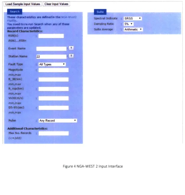
As discussed at the beginning of this section, we use the NGA-West 2 database to access earthquake records. Since the database has a tremendous volume of ground motion data for San Francisco area, we only consider the data recorded by the San Francisco Fire Department ground-motion recording station. The input parameters of the NGA-West 2 interface for target data are listed below:
RSN Event Name Station Name Fault type Magnitude RJB (km) R-rup (km) Vs30 (m/s) D5-95 (sec)
N/A1; since we are finding multiple data sets instead of a specific data set,
this section is left blank
N/A; since there are multiple faults within the area and the purpose of
sourcing data is finding all possible earthquake events happened in the previous, this section is left blank
22 Golden; since we are looking for ground motion records from the San Francisco Fire Department ground motion recording station only, the station needs to be specified in the input section. "22 Golden" is the first chunk of characters in the station's name string
N/A; since we are interested in frequency content of seismic data at a specific
site, the fault type does not need to be specified. And therefore, this section
is left blank
N/A; since all earthquakes will be scaled to produce equivalent results, this
section is left blank for all possible past events
N/A; No specific fault is chosen N/A; No specific fault is chosen
N/A; No specific earthquake magnitude is chosen N/A; No specific earthquake magnitude is chosen
Chapter 2. Frequency Content Analysis
Pulse N/A; No specific earthquake type is chosen
NGA-West 2 database provides a suite of spectrum analysis when searching for ground motion records. Since we are not using the spectrum provided by NGA-West 2, the input parameters for the suite section are randomly chosen. Figure 4 shows the interface of NGA-West 2 with input parameters listed above.
New Search
Load
~
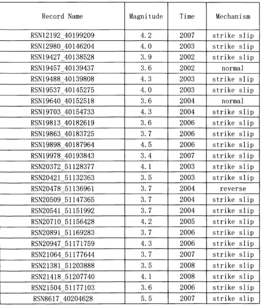
Ak Sm np VLus rG1!vnp auwsBased on the searching with input parameters above, we are able to locate total of 25 ground motion data sets recorded by the San Francisco Fire Department recording station dated from
2003 to 2008, and each record represents a unique event. Out of 25 ground motion records,
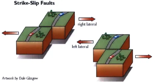
22 of them are generated by the strike slip fault type. Strike slip faults are vertical or nearly vertical fractures (as shown in Figure 5) where two pieces of earth next to each other move horizontally or nearly horizontally. Strike slip is the most common fracture plane in California, and therefore the ground motion data obtained from NGA-West 2 is representative. Table 1 below summarizes the records obtained from NGA-West 2 with earthquake mechanism
specified.
Record Name Magnitude Time Mechanism
RSN12192_40199209 4.2 2007 strike slip RSN12980_40146204 4.0 2003 strike slip RSN19427_40138528 3.9 2002 strike slip RSN19457_40139437 3.6 2002 normal RSN19488_40139808 4.3 2003 strike slip RSN19537_40145275 4.0 2003 strike slip RSN19640_40152518 3.6 2004 normal RSN19703_40154733 4.3 2004 strike slip RSN19813_40182619 3.6 2006 strike slip RSN19863_40183725 3.7 2006 strike slip RSN19898 40187964 4.5 2006 strike slip RSN19978_40193843 3.4 2007 strike slip RSN20372_51128377 4.1 2003 strike slip RSN20421_51132363 3.5 2003 strike slip RSN20478_51136961 3.7 2004 reverse RSN20509_51147365 3.7 2004 strike slip RSN20541_51151992 3.7 2004 strike slip RSN20710_51156428 4.2 2005 strike slip RSN20891_51169283 3.7 2006 strike slip RSN20947_51171759 4.3 2006 strike slip RSN21064_51177644 3.7 2007 strike slip RSN21381_51203888 3.5 2008 strike slip RSN21418_51207740 4.1 2008 strike slip RSN21504_51177103 3.6 2006 strike slip RSN8617 40204628 5.5 2007 strike slip
Chapter 2. Frequency Content Analysis
Strike-Slip Faults
right lateral
left lateral
Artwork by Dale Glasgow
Figure 5 Strike Slip Fault (Nevada Seismological Lab)
As discussed earlier in this section, ground acceleration data is the only measurement we take into account. Also, we ignore vertical ground acceleration for the scope of this thesis. Since-horizontal ground acceleration is measured in two directions, North-South and West-East, it is practical to aggregate two measurements into a single acceleration record. In order to merge two acceleration records, we apply Square Root of Sum of Square (SRSS) method to compute the single acceleration record. The theory behind aggregating acceleration file and its advantages are listed below:
" Ground motion acceleration records are measured at a fixed point, i.e. a specified
recording station. The directions of the acceleration records depend on the orientation of the recording station as well as the orientation of the recording instruments. In order to produce analysis results that can be applied without restrictions on structure orientation, acceleration records in two directions need to be combined into one acceleration record. And then, the combined acceleration record can be applied from both directions of the structure in later structural analysis part in chapter 3.
" Response spectrum of the structure requires single sided record data. By aggregating
acceleration records, we ultimately create the single sided acceleration record that can be applied later in the structural analysis part.
SRSS is a rapid and efficient way of combining records. It takes the sum of square of two parameters, and the positive result of the square root of the sum is the target value. In our case, we take the sum of square of ground acceleration records from both directions at each time step, and the square root of the sum is the aggregated acceleration record. The sampling frequency of NGA-West 2 database is 100 Hz, meaning the time step is 0.01 sec. The time interval of each record lasts from 200 seconds up to 360 seconds depending on the event. And therefore, each data record contains a considerable amount of sampling points, ranging from 20,000 points to 36,000 points. Computation efficiency is significant, and thus SRSS is ideal for the scope of our analysis for its high performance cost ratio. By applying SRSS, the total
operations for both data processing and structural analysis are cut in half. The SRSS function and its parameters are defined in equation 2-3 as follows:
iiagg N E (2-3)
where iagg aggregate acceleration [ft/s2]
NS acceleration in North-South direction [ft/s2
UWE acceleration in West-East direction [ft/s2
In order to obtain a more intuitive understanding of the ground motion activities, we utilize Matlab to plot time history diagrams from the aggregated acceleration. As discussed before, computational efficiency is significant in our analysis, and Matlab is ideal for analyzing data with intensive sampling data points. Also, Matlab is the most suitable solution for repetitive computations, which is the case for plotting time history diagrams for different data sets. In addition, by applying a plot feature of Matlab, we are able to filter out noise and aftershock portions of the data. Selected time history diagrams for ground acceleration are shown below in Figure 6, and the remaining are shown in Appendix A. The unit for measuring ground acceleration in NGA-West 2 database is in percentage of gravitational acceleration, meaning the Y-axis of time history diagrams shows the magnitude of acceleration in percentage of gravitational acceleration, while X-axis shows the time [s].
Chapter 2. Frequency Content Analysis 0012 0.01 0.008 0.006 8 0,004 0002 50 100 150 200 250 300 350 400 Time (s)
Single Sided Acceleration Diagram
RSN20541 0.14 0-12 0.1 0.08 8006 0.04 0.02
Single Sided Acceleration Diagram
RS#4e17 008
v
0.07 006 005 004 003Single Sided Acceleration Diagram
L
015r 01 8 005k 0 50 100 150 200 25 Time (s)10-3 Single Sided Acceleration Diagram
I
6 4 8 3 2j. Time (s) 0Single Sided Acceleration Diagram
RSN12teO
L
L
o -
-0 20 40 60 80 100 120 140 160 180 200 Time (s)
10-3 Single Sided Acceleration Diagram
-- R8N16537 -- RI2I5J 2.5 2 8 <1 05 200 250 0 50 100 150 200 250 300 350 40 Trpm (S)
Figure 6 Selected Time History Acceleration
~~LJL
nL-J 0 0.02 0010
a 0 50 100 150 200 250 300 350 400 Time (s) I 02.3.2 Records Set Filtering
Time history data plots in the precious section provided an intuitive view of the ground motion activities. Keep in mind, the ground acceleration records plotted above are single sided as a result of aggregating accelerations in both directions. Also, single sided acceleration records have no impact on the performance of structures. And therefore, single sided acceleration records are valid to be utilized within the scope of this thesis. Ground acceleration time history records plotted above are summarized as three categories as follow:
E Pulse like wave function. This type of earthquake has one major pulse in the ground motion acceleration plot. And the magnitude of the pulse is significantly larger than the rest ups and downs of the wave function. Pulse like ground motion is the most typical ground motion activity, which produces one significant shake with a bunch of small vibrations.
0 Two-pulse wave function. This type of earthquake has two major pulses follow each
other in the ground motion acceleration plot. And the difference in magnitude between these two pulses is relatively small compares to the difference with the rest ups and downs of the wave function. Two-pulse ground motion is similar to a pulse like ground motion follows by another pulse like ground motion within a short time interval.
N Multi-pulse wave function. This type of earthquake has multiple major pulses follow each other in the ground motion acceleration plot. Each pulse is accompanied by a series of smaller vibrations. Multi-pulse like ground motion is not a typical wave function in our analysis.
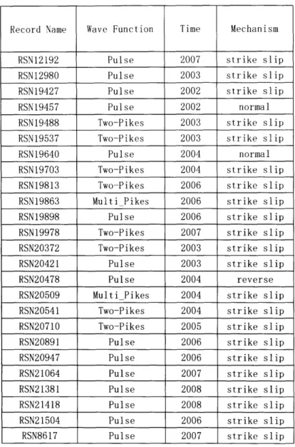
In Table 2 ground acceleration records are summarized in terms of shape of wave function, also, corresponding fault types are listed as well for later analysis and comparison. According to our summary, out of 25 ground acceleration records, 15 are pulse like ground motion activities, 8 are two pike pulse like ground motion activities, and the other 2 are multi-pulse ground motion activities. For our scope of analysis, in order to limit the variables other than frequency related parameters, we eliminate multi-pules ground motion in later analysis. As for two pulse ground motion activities, we tend to eliminate noise manually as much as possible, and the same ideology applies to pulse like ground motion activities as well. Also, the lengthy recording time results in delays in structural analysis computation time. For the consideration of computation efficiency, tails of acceleration records with negligible magnitudes are deleted manually.
Chapter 2. Frequency Content Analysis
Record Name Wave Function Time Mechanism
RSN12192 Pulse 2007 strike slip
RSN12980 Pulse 2003 strike slip
RSN19427 Pulse 2002 strike slip
RSN19457 Pulse 2002 normal
RSN19488 Two-Pikes 2003 strike slip
RSN19537 Two-Pikes 2003 strike slip
RSN19640 Pulse 2004 normal
RSN19703 Two-Pikes 2004 strike slip
RSN19813 Two-Pikes 2006 strike slip
RSN19863 Multi Pikes 2006 strike slip
RSN19898 Pulse 2006 strike slip
RSN19978 Two-Pikes 2007 strike slip
RSN20372 Two-Pikes 2003 strike slip
RSN20421 Pulse 2003 strike slip
RSN20478 Pulse 2004 reverse
RSN20509 MultiPikes 2004 strike slip
RSN20541 Two-Pikes 2004 strike slip
RSN20710 Two-Pikes 2005 strike slip
RSN20891 Pulse 2006 strike slip
RSN20947 Pulse 2006 strike slip
RSN21064 Pulse 2007 strike slip
RSN21381 Pulse 2008 strike slip
RSN21418 Pulse 2008 strike slip
RSN21504 Pulse 2006 strike slip
RSN8617 Pulse 2007 strike slip
Record Name Wave Function Mechanism (Data Points)
RSN12192 1600-6000 Pulse strike slip
RSN12980 2000-6000 Pulse strike slip
RSN19427 2000-6000 Pulse strike slip
RSN19457 1600-6000 Pulse normal
RSN19488 5000-10000 Two-Pikes strike slip
RSN19537 5000-10000 Two-Pikes strike slip
RSN19640 5000-10000 Pulse normal
RSN19703 5000-10000 Two-Pikes strike slip
RSN19813 5000-10000 Two-Pikes strike slip
RSN19898 5000-10000 Pulse strike slip
RSN19978 5000-10000 Two-Pikes strike slip
RSN20541 1-6000 Two-Pikes strike slip
RSN20710 1000-6000 Two-Pikes strike slip
RSN20891 1-5000 Pulse strike slip
RSN20947 2000-6000 Pulse strike slip
RSN21064 2000-5000 Pulse strike slip
RSN21381 1-4000 Pulse strike slip
RSN21418 1-5000 Pulse strike slip
RSN21504 1-5000 Pulse strike slip
RSN8617 1000-6000 Pulse strike slip
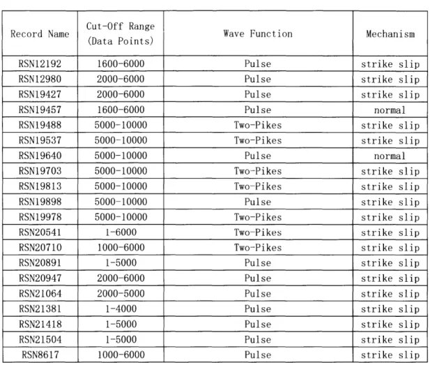
Table 3 Cut off Range
Table 3 summarizes the cut off range of data points for the ground motion acceleration data records plotted above. There are total of 25 data sets accessed from NGA-West 2 database, and they can be combined into 3 different wave function categories as mentioned above. Several data sets are eliminated randomly to minimize the volume of necessary data sets. Also, cut-off points for data sets are determined intuitively for the purpose of eliminating blank values or negligible values. Filtered time history plots for ground motion acceleration are plotted with Fourier transform diagrams in section 2.3.3.
Chapter 2. Frequency Content Analysis
2.3.3 Frequency Content of Seismic Data
As mentioned in section 2.2, fast Fourier transform is used in our analysis to transfer ground acceleration records from time space to frequency space. Considering the large amount of sampling points in our data sets, we have to use numerical tools computing Fourier transforms. Matlab has a built-in function that computes fast Fourier transform automatically. Also, Matlab is efficient in terms of plotting and handling large volume of data, and thus, we use Matlab to compute fast Fourier transform.
Matlab's built-in fast Fourier transform function uses Cooley-Tuckey method computing discrete Fourier transform. The function and its implementation are listed below in equation 2-4:
Y = ff t(X, n) (2-4)
where Y n-point Discrete Fourier Transform
n size of X
X matrix of original data in time space
ff t(X, n) Fast Fourier Transform operation command
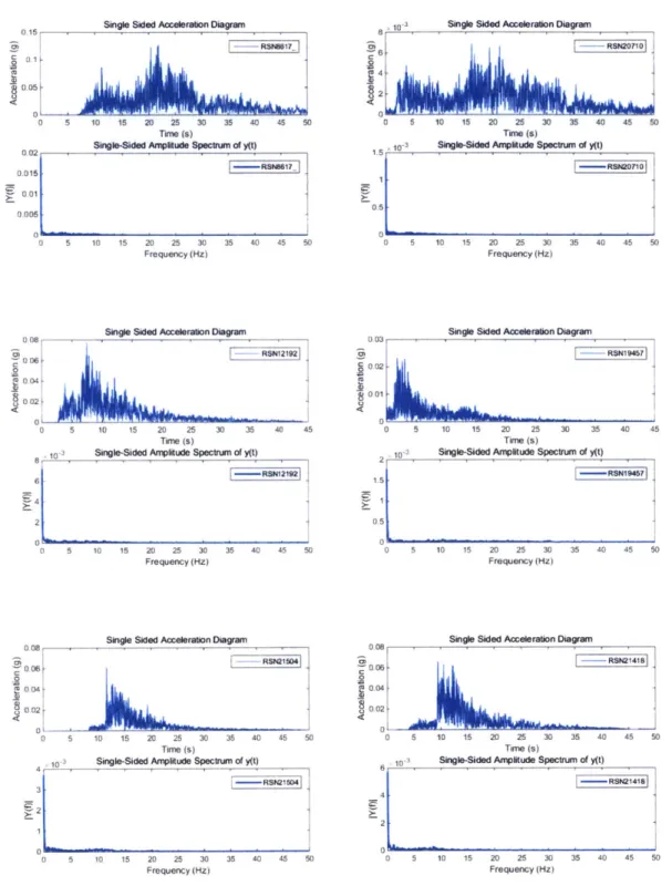
As mentioned in section 2.2, Cooley-Tuckey method's computation efficiency is limited by the power of two size of sampling points. Meaning, the count of data points must be power of two. In order to take advantage of the computation efficiency, we deliberately make n, size of X, the next power of two. And we will only plot the discrete Fourier transform up to the signal length at the end. Selected filtered time-history ground acceleration diagrams are plotted in Figure 7, along with corresponding discrete Fourier transform diagram. The remaining filtered time-history ground acceleration diagrams with corresponding discrete Fourier transform diagrams are attached in Appendix A.
Single Sided Acceleration Diagram 10-3 Single Sided Acceleration Diagram RSN0) 17- RSN20710 S 0.1- 4-0105 02 0 5 10 15 2D 25 30 35 40 45 50 0 5 10 15 20 25 30 35 40 45 50 Time (s) Time (s)
Single-Sided Amplitude Spectrum of y(t) 10-3 Sngle-Sided Amplitude Spectrum of y(t)
0.02 1. ,t5 - RSW17 0_ 11 0 01 0.006 0 0 5 10 15 20 25 30 35 40 45 50 Frequency (Hz)
Single Sided Aceleration Diagram
0 06 RSNI2192
0 02
0 5 10 15 20 25 30 35 40 45
Time (s)
10-3 Single-Sided Amplitude Spectrum of y(t)
--- RSN121921 e 1 4 2 1 0 O 5 10 15 20 25 30 35 40 45 50 Frequency (Hz) 0 -. 0 5 10 15 20 25 30 35 40 45 50 Frequency (Hz) 0 02 001
Single Sided Awceleration Diagram
0 5 10 15 20 25 30 35 40 45
Time (s)
, 10-3 Single-Sided Amplitude Spectrum of y(t)
15
0 5
0 5 10 15 20 25 30 35 4A 45 so Frequency (Hz)
Single Sided Aoceleratlon Diagram
0 D8 i 0)
~RSNr2lO4j
~
0. 0134
0 04 0 02 01 0 5 10 15 20 25 30 35 40 45 50 Time (s)10-3 Single-Sided Amplitude Spectrum of y(t) - RSN21504
2
0 5 10 15 20 25 30 35 40 45 50
Frequency (Hz)
Single Sided Acceleration Diagram
0 08 -- RSN2 1418 0 WI 2004 0.02 0 5 10 15 20 25 30 35 40 45 50 Time (s)
-in' Single-Sided Amplitude Spectrum of y(t)
4 2
-RS5~i418
0 5 10 15 20 25 30 35 40 45 50
Frequency (Hz)
Figure 7 Selected Discrete Fourier Transforms
0
15Chapter 2. Frequency Content Analysis
The Discrete Fourier transforms illustrated above include different types of ground motion acceleration data records. The maximum acceleration for all ground acceleration records happens at 0 Hz, and the acceleration drops dramatically after that. After dropping to its average level, the acceleration gradually dies out. The variation of acceleration after initial high points tend to differentiate one data record from another. Although the difference in accelerations at different frequencies is relatively small, the trend of variation between high frequency accelerations and low frequency accelerations can be observed. Therefore, discrete Fourier transforms are analyzed without initial high points in acceleration. Figure 8 shows the discrete Fourier transforms of ground motion acceleration data for selected ground motion records without initial high points.
Single Sided Acceleration Diagram
015
0.05
0 5 10 15 20 25 30 35 40 45 50
Time (s)
1-3 Single-Sided Akude Spectrum of y(t) cut-off
1-5 1
->- Rdf6lJ7
0.5
0 5 10 15 20 25 30 35 40 45 50
Frequency (Hz)
Single Sided Acceleration Diagram
-M RSN1I2192
004
S0 02
0 5 10 15 20 25 30 35 40 45
Time (s)
8 10-1 Single-Sided Amplitude Spectrum of y(t) cit-off
S - RSN12a2
j
-4
2
0 5 10 15 20 25 30 35 40 45 50
Frequency (Hz)
1o4 Single Sided Acceleration Diagram 8 1 IRSaN20710 0 S2 0 5 10 15 20 25 30 35 40 45 50 Time (s)
10 dd A ude Specu cut-off
-- R20710
05
0.
0 5 10 15 20 25 30 35 40 45 50
Frequency (Hz)
Single Sided Acceleration Diagram
11'RSNIa451
002
0 01
0 5 10 15 20 25 30 35 40 45
Time (s)
10 Single-Sided Amplitude Spectrum of y(t) cut-off
3 RSN1B45
0 5 10 15 20 25 30 35 40 45 50
Frequency (Hz)
The plots above with cut-off discrete Fourier transforms clearly show the acceleration trends in terms of frequency, and the plots for rest of ground motion data sets are listed in Appendix
A. By excluding initial high points, acceleration variations with frequency are clear.
Although cut-off discrete Fourier transforms have a considerable amount of noise due to complexities in the nature of ground motion activities, relative trend within the diagram is obvious. According to the data analyzed above, most ground accelerations are peaked at two different frequency ranges, namely, 1-3 Hz and 7 Hz. However, as observed in the diagrams above, frequencies other than the two ranges mentioned before are having significant impact on the behavior of ground acceleration.
2.4 Summary
This chapter completes the frequency content analysis. We use ground motion acceleration data obtained from NGA-West 2 database to perform frequency content analysis using fast Fourier transform. The data accessed are site specific, all data are recorded by San Francisco Fire Department Recording Station. In order to accomplish the analysis task as well as maintaining consistency and applicability of our analysis results, accelerations in two horizontal directions are aggregated into one acceleration that can be applied later in the structural response analysis. And time history diagrams for acceleration are plotted in
As mentioned in section 2.3, we cut-off negligible acceleration values to promote computation efficiency. Discrete Fourier transforms are computed based on filtered data. However, as we can see from Figure 7, initial high points of acceleration values skewed the Fourier transforms. By eliminating initial high points, we are able to produce relatively clear
acceleration trend based on frequency. The accelerations in frequency domain can be summarized of having frequency concentration range of 1-3 Hz and 5-7 Hz.
The reasons why discrete Fourier transforms display the very phenomenon are as follow:
* Initial high points at low frequency contents are visualized due to complexity in the nature of seismic data. Discrete Fourier transform establishes a frequency domain for time history functions, and it decomposes time domain functions into a combination of predetermined sinusoidal functions with corresponding coefficients. However, since seismic activities are extremely complex, discrete Fourier transforms of seismic data are hard to compute. The practical way of computing Fourier transforms is setting high initial values and modifying it with numerous functions.
* As we can observe from the cut-off spectrum diagrams, the variation between frequencies are clear but small. Meaning, sinusoidal functions with different frequency characteristics affect the overall behavior of the ground motion. However,
Chapter 2. Frequency Content Analysis
some sinusoidal functions with frequency ranges from 1-3 Hz or 5-7 Hz are weighted more in terms of frequency content than that of other sinusoidal functions
Chapter 3. Non-Structural Damage Assessment
A method to determine structural response is presented in this chapter and followed by a
discussion of evaluating non-structural damage of a target building. Finite element analysis method is utilized to determine structural response criteria including accelerations and displacements of the target structure.
3.1 Introduction
The section introduces the target structure to be analyzed and the approach used to evaluate non-structural damage. All ground motion acceleration data used in this section are obtained
from the results in chapter 2. The data applied in this chapter include filtered ground motion acceleration records, which are produced at the end of chapter 2. Also, the ASCE 7-10 response spectrum is used to scale ground motion acceleration records.
3.1.1 Sample Structure
A sample structure is designed in section 3.2 to be analyzed for performance under ground
motion activities. Since this thesis focuses on site specific structural response, the site chosen for analysis is San Francisco, Bay Area. All data accessed in this thesis are obtained from
NGA-West 2 database, and the recording station is San Francisco Fire Department recording station. The recording station is located in 22 Golden Gate Park as shown in Figure 2, and as we can see, the recording station is located in a highly populated area near downtown San Francisco. According to the picture, the typical building type in San Francisco is low rise residential, mixed-use and office buildings. Considering the fact that this thesis is performed to evaluate non-structural damage induced by seismic activities, which is applicable to the majority of residents in San Francisco, we decide to design a typical office/residential/mixed use low rise building for later use. Therefore, the sample structure is determined to be a 5
story 70 ft tall building with 5 bays by 6 bays in plan. The side view of the building is shown in Appendix C, more details about the design process are carried out in section 3.2.
3.1.2 Chapter Objectives and Organization
This chapter discusses the finite element analysis of the structural performance under seismic activities. Then the results obtained from the structural analysis are utilized in determining non-structural damage assessment. The objectives of this chapter are: 1) Design a target structure which is representative of residential/office/mixed-use structures in San Francisco; 2) Evaluating structural response under seismic activities summarized in Chapter 2.
Chapter 3. Non-Structural Damage Assessment
This chapter first illustrates the design procedures of the target structures as well as sizing procedures in section 3.2. And in section 3.3, detailed ground motion records scaling process and structural response analysis are discussed in detail. Finally, section 3.4 talks about the structural response results and demonstrates the non-structural damage assessment based on the results.
3.2 Sample Structure Design
As mentioned in section 3.1.1, the target structure is set to be a 5 story 70 ft height building with 5 bays by 6 bays in plan. The structure is selected based on the consideration of representativeness of typical residential/office/mixed use buildings in San Francisco Area. This section provides basic assumptions for the structural design as well as detailed gravity design procedures. The reason for gravity design only is discussed in this section as well.
3.2.1 Design Assumptions
The target structure is selected to represent typical residential/office/mixed-use structures in San Francisco Area. Several assumptions for the structure in terms of location and design are listed below:
" The proposed location for the structure is at 22 Golden Gate Park, which is the location
for the recording station where all data used in this thesis are recorded. Since this thesis focuses on the seismic induced structural impact on a site specific basis, analyzing a target structure at the specific site where data are recorded is ideal for minimizing non-controllable effects of our analysis. Also, the 22 Golden Gate Park is located close to downtown San Francisco, which is a representative location for typical residential/office/mixed-use buildings.
" The structural design of this building follows ASCE 7-10 building code. However,
safety factors for load determination and capacity determination are ignored. This thesis focuses on comparison analysis between ground motion activities with different frequency content, and therefore we are only using relative results instead of absolute results. Based on this consideration, minimum design criteria is sufficient for the design process
* The structural design only considers gravity design. Meaning, no lateral system is specifically designed for the structure. The structure is designed with gravity members only, and all members are sized with gravitational force considerations only.
Two way slabs are designed to transfer load to beams, and beams are designed based on tributary area method. Also, columns are designed using tributary area method as well. Columns are assumed to be rigid and fixed at the ground support. The overall structural system of the building is assumed to be a frame system. The frame
system, however, is not specifically designed to satisfy any lateral design criteria.
0 The building utilizes steel beams and columns with typical concrete floor slabs. Steel structure is chosen based on two considerations: 1) steel structures have high ductility, and thus steel structural behaviors are more predictable under low magnitude earthquake events; 2) steel structures are easier to implement in finite element analysis model, and using steel structures will promote computation efficiency.
3.2.2 Simplified Gravity Design
The simplified gravity design for the target structure is illustrated in this section. The design procedure is decomposed into two parts, namely, load determination and member sizing. Also, for each part, the computation is separated into parts in terms of member types. The Design procedure is detailed once only for each type of structural member for illustration, and other members are designed the same way.
Member Size
Beam W44X335
W8X31 Column
W8X48
Chapter 3. Non-Structural Damage Assessment
The parameters used in the load determination process are defined below:
a distributed load demand [psf]
WL line load [k/f]
AT tributary area [ft2]
PD demand load [kip]
Pc member capacity [kip]
L length [ft]
w width [ft]
MN nominal moment [kip -ft]
MD moment demand [kip -
ft]
0 reduction factor Typical Beam: a = 200 psf2 AT = 22 ft x 22 ft = 484 ft2 CO = 22 ft x 200 psf = 4.4 kf WL x MD =266.2 kip ' ft 8 0MN > MD3
Select W44 x 335 from AISC Steel Manual
2 Distributed load is set to be 200 psf arbitrarily to match typical distributed load for residential/office/mixed-use
buildings
3 As mentioned in Section 3.1, we ignore factor of safety in the design procedure, and therefore the reduction factor 0 is
Typical Column:
w = 200 psf
AT = 22
ft
x 22ft
= 484 ft 2PD= x AT = 96.8 kips
Check for Buckling
12 x E x I
Pcr (KL) 2
where Pcr critical load to induce buckling [kip]
E Young's modulus [ksi]
I moment of inertia [in']
KL effective length [f t]
Select W 8 x 31 from AISC Steel Manual
There are two member sizes used for columns. The first column size is W 8 x 31, which is applicable to columns above first floor. The second column size is W 8 x 48, which is applicable to columns between ground floor and first floor.
3.3 Structural Response
This section performs structural analysis on the target structure, and the response under ground motion activities are determined using data prepared in chapter 2. This section first develops a virtual Single Degree of Freedom structure with natural frequency equivalent to first failure mode frequency of the target structure. And the ground motion records are scaled with respect to ASCE 7-10 response spectrum at the period corresponding to the first failure mode frequency. After obtaining scaled seismic records, we use the finite element analysis model to determine corresponding displacements and acceleration parameters.
3.3.1 SDOF
A virtual SDOF model equivalent to the first dynamic mode of the target structure is developed
in this section for the purpose of scaling ground motion acceleration records. In order to obtain the frequency for the first dynamic mode of the target structure, we used the finite element analysis model before conducting structural response analysis under seismic activities. And therefore, we borrowed dynamic analysis results in terms of modal analysis. More detail
Chapter 3. Non-Structural Damage Assessment
about finite element model implementations and performing analysis are discussed in section 3.3.3
As determined from the finite element analysis model, frequency for the first failure mode of the sample structure is 0.2716 Hz, and the corresponding period is 3.682 sec. The dynamic mode is shown in Figure 9. With the first dynamic mode frequency known, we are able to scale acceleration records with respect to the ASCE 7-10 spectrum.
SCAe 1 47.7 Woleto ScaleI 1W 5 7 ll~gtigted Ccaeo Modes Cocoteo Eleoet DeforowaOm resofcto 5000 Cane A I Oyoos MOdelI
mode 1
Freqoeocy 0.2716m,-Pered 3 6V s
A
Figure 9 Sample Structure First Dynamic Mode
3.3.2 Seismic Data Scaling
As mentioned in section 2.1, we are using unscaled time history ground motion data from NGA-West 2 database although the scaled response spectrum are provided. The reason for using unscaled data is due to the consideration of the site-specific feature of our analysis. The scaled response spectrum provided by NGA-West 2 minimizes the differences between target spectrum and scaled spectrum over a range of periods. This method is ideal for analyzing the response of structures under multiple dynamic modes, and it will provide more reliable results. However, the scaling method utilized by NGA-West 2 is very computationally expensive, and it will not provide us with a desired result under the scope of our analysis.
Since we are analyzing non-structural damage under seismic activities for the target building, no permanent structural damage will be considered. For most structures, the number of dynamic modes to be analyzed very much depends on the type of analysis to be performed. The most typical dynamic modes analysis utilizes are the first three modes, while the first mode