HAL Id: tel-01112334
https://tel.archives-ouvertes.fr/tel-01112334
Submitted on 2 Feb 2015HAL is a multi-disciplinary open access
archive for the deposit and dissemination of sci-entific research documents, whether they are pub-lished or not. The documents may come from teaching and research institutions in France or abroad, or from public or private research centers.
L’archive ouverte pluridisciplinaire HAL, est destinée au dépôt et à la diffusion de documents scientifiques de niveau recherche, publiés ou non, émanant des établissements d’enseignement et de recherche français ou étrangers, des laboratoires publics ou privés.
Tuan Minh Pham
To cite this version:
Tuan Minh Pham. Formal Description of Geometrical Properties. Logic in Computer Science [cs.LO]. Univeristé Nice Sophia Antipolis, 2011. English. �tel-01112334�
´
ECOLE DOCTORALE STIC
SCIENCES ET TECHNOLOGIES DE L’INFORMATION ET DE LA COMMUNICATION
T H E S E
pour obtenir le titre de
Docteur en Sciences
de l’Universit´
e de Nice - Sophia Antipolis
Sp´
ecialit´
e : Informatique
Pr´esent´ee et soutenue par
Tuan-Minh PHAM
Description formelle de
propri´
et´
es g´
eom´
etriques
Th`
ese dirig´
ee par Yves BERTOT
et pr´
epar´
ee `
a l’INRIA Sophia Antipolis, projet Marelle
soutenue le 21 Novembre 2011 Jury :
Jean-Fran¸cois Dufourd - Universit´e de Strasbourg (Rapporteur) Julio Rubio - Universit´e de La Rioja (Rapporteur) Jacques Fleuriot - Universit´e de ´Edimbourg (Examinateur) Julien Narboux - Universit´e de Strasbourg (Examinateur) Yves Bertot - INRIA-Sophia Antipolis (Directeur)
La g´eom´etrie synth´etique, aussi parfois appel´ee g´eom´etrie axiomatique, s’int´eresse purement aux objets g´eom´etriques. En reposant sur des ax-iomes et des th´eor`emes qui mettent en relation les concepts de base de la g´eom´etrie, elle permet de mettre en valeur les propri´et´es g´eom´etriques pendant les preuves math´ematiques.
Cette th`ese se concentre sur les propri´et´es g´eom´etrique et leur description dans le syst`eme de preuve Coq. Les deux r´esultats principaux sont une biblioth`eque de descriptions formelles et une extension du syst`eme de preuve pour permettre une interaction directe avec les objets g´eom´etriques pendant les preuves.
La premi`ere partie pr´esente notre formalisation de la g´eom´etrie euclidienne bas´ee sur la g´eom´etrie affine. Nous approchons les notions, les propri´et´es, et les th´eor`emes dans un style similaire `a celui utilis´e dans l’enseignement au lyc´ee. Notre d´eveloppement am´eliore le d´eveloppement fourni pr´ec´ edem-ment par F. Guilhot en ´eliminant les axiomes inutiles, en fournissant des d´efinition mieux appropri´ees pour certains objets g´eom´etriques, et en re-formalisant leurs propri´et´es.
La deuxi`eme partie s’int´eresse `a la question de l’orientation dans le plan. Cela permet d’enlever certaines ambigu¨ıt´es dans la pr´esentation des objets g´eom´etriques et d’´enoncer des probl`emes de g´eom´etrie ”ordonn´ee” et de les prouver.
La troisi`eme partie s’int´eresse `a des questions de fondement. En particulier, nous montrons que les syst`emes d’axiomes de Hilbert et Tarski peuvent ˆ
etre mod´elis´es dans notre syst`eme. Nous montrons ´egalement que notre syst`eme d’axiome peut supporter les outils de preuve automatique bas´es sur la m´ethode des aires ou sur les bases de Gr¨obner. Le travail sur les bases de Gr¨obner a ´et´e effectu´e en collaboration avec J. Narboux.
Coq avec l’outil de g´eom´etrie dynamique GeoGebra, en se reposant sur l’interface d’utilisation pour Coq d´evelopp´ee en Java et appel´ee Pcoq. Le r´esultat de cette combinaison permet aux utilisateurs d’effectuer facilement des raisonnements g´eom´etriques dans le style de la g´eom´etrie du lyc´ee, in-teractivement et avec le support d’une interface graphique. Ceci montre comment un syst`eme de preuve pourrait ˆetre utilis´e en ´education.
Mots-clefs: Formalisation de la g´eom´etrie, Preuve interactive, Coq, logiciel de g´eom´etrie dynamique.
Synthetic geometry, sometimes also called axiomatic geometry, deals purely with geometric objects. Relying on axioms and theorems relating the basic concepts of geometry makes it possible to highlight the geometrical proper-ties during the proofs.
This thesis concentrates on geometrical properties and their description in the Coq proof assistant. The two main results of this thesis are a library of formal descriptions and a proof system extension to interact directly with geometrical objects during proofs.
The first part presents our formalization of Euclidean geometry based on affine geometry. We approach notions, properties, and theorems in a style similar to what is taught in high school. This development improves on the library developed by F. Guilhot by eliminating needless axioms, giving more appropriate definitions for some geometric notions and re-formalizing their properties.
The second part deals with the notion of orientation in the plane. It allows us to remove ambiguities in the presentation of geometric objects and state and solve ordered geometry problems.
The third part deals with foundations. In particular, we show that the axiom systems of Hilbert and Tarski can be described on top of ours. We also show that automatic proof methods like the area method and Gr¨obner bases can be integrated. The work on the area method was performed jointly with J. Narboux.
The fourth part presents a combination of the Coq formal proof tool and the Geogebra dynamic geometry tool. This is based on the java-based user-interface for Coq named Pcoq. This combination allows users to easily perform geometry reasoning as taught in high school and in a interactive manner with the support of a graphic interface. This shows how a proof system could be used in education.
Contents
1 General Introduction 1
1.1 Teaching and learning geometry . . . 1
1.2 Using dynamic geometry software . . . 3
1.3 Formal proof with a proof assistant . . . 4
1.4 Our work . . . 5
2 Formalization of Elementary Geometry 6 2.1 Introduction . . . 6
2.2 A formalization of high-school geometry . . . 8
2.3 Reducing axioms and having a constructive library in a geometric view . 12 2.4 Formalization of affine geometry . . . 13
2.4.1 Formalization of vector . . . 16
2.4.2 Formalization of line . . . 22
2.5 Formalization of Euclidean geometry . . . 26
2.5.1 Cartesian coordinate system . . . 28
2.5.2 Elementary constructions . . . 31
2.5.3 Compound constructions . . . 33
2.5.4 Angle and Trigonometry . . . 34
2.5.5 Plane transformation . . . 38
2.6 Discussion . . . 39
2.7 An example about school proof and formal proof . . . 41
2.7.1 The proof in school . . . 42
2.7.2 The formal proof . . . 42
2.7.3 Discussion . . . 45
3 Orientation and its applications 47
3.1 Introduction . . . 47
3.2 Definition of orientation . . . 49
3.3 Some properties of orientation . . . 50
3.3.1 The properties of Knuth’s system . . . 50
3.3.2 Proving the properties . . . 51
3.3.3 Variants . . . 56
3.4 Orientation and order . . . 56
3.4.1 Properties . . . 56
3.4.2 Proving the properties . . . 59
3.5 Some application . . . 61
3.5.1 Orientation in formalizing some geometric notions . . . 61
3.5.2 Orientation in Proving Theorems . . . 67
3.6 Some discussions about full angles . . . 70
3.7 Conclusion . . . 71
4 Multiple Points of View about Geometry 72 4.1 Introduction . . . 72
4.2 Verifying axiomatic systems of synthetic geometry . . . 73
4.2.1 Verifying Hilbert’s system . . . 73
4.2.2 Verifying Tarski’s system . . . 81
4.3 Combining with the area method . . . 82
4.3.1 The area method . . . 82
4.3.2 Correctness of the area method . . . 85
4.3.3 Usability of the area method . . . 88
4.4 Combining with the method of Gr¨obner bases . . . 95
4.5 Conclusion and future work . . . 97
5 Dynamic Geometry Tool for Interactive Theorem Proving 99 5.1 Context . . . 99
5.2 Introduction to Geogebra . . . 101
5.3 Some analyses about school proofs . . . 103
5.4 The interface with the proof related feature . . . 105
5.4.1 A snapshot of the interface . . . 105
5.4.2 Stating theorems . . . 106
5.5 Some discussion about proving with our interface . . . 114
5.6 Communication between Geogebra with Coq . . . 114
5.7 Implementation . . . 115
5.7.1 Integration of the prove view . . . 116
5.7.2 Tree structure for geometric object definition . . . 117
5.7.3 Interactions with users during their proofs . . . 118
5.7.4 Visualizing theorem statements . . . 120
5.8 Conclusion and Future Work . . . 120
6 General Conclusion and Perpectives 122 6.1 Conclusion . . . 122
6.2 Perspective . . . 123
A Formal proof of a geometry theorem 126
General Introduction
1.1
Teaching and learning geometry
Geometry is an important branch of mathematics, that deals with properties, mea-surement and relationships between geometric objects. Learning geometry is a brain-boosting activity that helps improve student’s brain function. Doing geometry proofs requires the brain to operate in new and complex ways. This requires logical thinking, a mental process that is rarely well developed in the younger students.
The conventional approach to geometry is synthetic or axiomatic geometry, which deals purely with geometric objects directly by geometrical properties. This is the kind of geometry, for which Euclid is famous, that makes use of axioms, theorems and logical arguments to draw conclusions. Its formal proofs are considered as sequences of geometric deductive reasoning from axioms. They are taught in high school with a well-known method called two-column method. A two-column geometric proof consists of a list of statements, and the reasons showing that those statements are true. The statements are listed in a column on the left, and the reasons for which the statements can be made are listed in the right column. Each reasoning step is a row in the two-column proof.
The use of formal proofs is always subject of debates for educators - see the survey of Battista & Clements [3]. Some argue that we should continue the traditional focus on axiomatic systems and proofs. Some believe that we should abandon proof for a less formal investigation of geometric ideas. Others believe that students should move gradually from an informal investigation of geometry to a more proof-oriented focus. High school geometry with its formal proofs is considered hard and very detached from practical life for some reasons: lack of proof and proving in earlier school years, lack of understanding of geometry concepts and student’s cognitive development.
The research of Piaget on student’s cognitive development shows that thinking in general progresses from being non-reflective and unsystematic, to empirical, and finally to logical-deductive. The research of Van Hiele on understanding of geometry concepts suggests that students’ geometrical understanding progresses through various levels in Tab.1.1.
◦ Level 1 - Visualization : Students can name and recognize shapes by their ap-pearance, but cannot specifically identify properties of shapes.
◦ Level 2 - Analysis : Students begin to identify properties of shapes and learn to use appropriate vocabulary related to properties, but do not make connections between different shapes and their properties.
◦ Level 3 - Argumentation : Students are able to recognize relationships between and among properties of shapes or classes of shapes and are able to follow logical arguments using such properties.
◦ Level 4 - Deduction : Students can go beyond just identifying characteristics of shapes and are able to construct proofs using postulates or axioms and definitions. A typical high school geometry course should be taught at this level.
Table 1.1: Students’ geometrical understanding progresses through various levels which cannot be skipped
Both theories suggest that students must pass through lower levels of geometric thought to attain higher level and that they can understand and explicitly work with axiomatic systems only after they have reached the highest levels. Thus, the explicit study of axiomatic systems is unlikely to be productive for the vast majority of students in high school.
Moreover, Battista and Clements suggest that the most effective way to include meaningful proof in classes is to avoid formal proof at the beginning and focus instead on justifying ideas based on visual and empirical foundations. This can gradually lead students to appreciate the need for formal proof. In fact, learning by inductive reasoning alone is ”surface learning” and deductive proof should continue to be an essential part of geometry curricula.
1.2
Using dynamic geometry software
Consistent with this alternative to axiomatic approaches, the focus of dynamic geome-try softwares (DGSs) is to facilitate students’ making and testing conjectures. Dynamic geometry softwares not only allow students to understand construction steps that lead to final drawings, but also provide access to geometric objects, allow students to move free points and observe the influence on the rest. This allows students to explore new implicit properties from the drawings. Some among the numerous dynamic geometry softwares provide a justification feature with the support of algebraic (coordinate-based) methods or semi-algebraic (coordinate-free) methods that facilitate justifying conjec-tures.
Nowadays, dynamic geometry softwares are widely used in school. Many researches pointed out the important role of dynamic geometry softwares in learning and teaching geometry. The use of dynamic geometry softwares can further students progress. The research on the influence of dynamic geometry softwares on students’ progress with respect to van Hiele levels [15][21] showed that dynamic geometry softwares may help students pass through van Hiele levels. However, most of the material proposed for the classroom seems to only be concerned with the first three levels.
The fourth level deals with deductive proof. In fact, algebraic (coordinate-based) methods or semi-algebraic (coordinate-free) methods only allows to justify conjecture. They do not offers a capability to build deductive proofs. In particular, algebraic methods are able to produce non-trivial geometric proofs automatically, but their proofs are usually long and hard to read. On the other hand, coordinate-free methods only use geometrically meaningful quantities and their generated proofs are human-readable. But these proofs still are not purely traditional deductive proofs, not produced in the manner taught in school.
The exploration and proof activities should be interlaced. I think that these two activities could be better interlaced if they were both conducted using the computer. This leads to the necessity of developing a geometry proving tool for high school students which they can use to to construct geometry object, explore conjecture and interactively construct traditional geometry proofs. Proving with a such system enables students to understand geometric concepts deeply and beyond the use of these concepts in scope of current being studied geometry problems.
1.3
Formal proof with a proof assistant
A proof assistant or interactive theorem prover is a tool to develop formal proofs guided by users. Proof assistants allow us to state mathematical theorems, perform logic reasonings and they verify the validity of logical steps.
Proofs are developed in a interactive manner that requires logical reasoning ca-pabilities from users. Therefore, using proof assistants could help students to better understand the concepts of deduction.
This use has more interest in proving geometry theorems because traditional geom-etry reasoning usually relies on tacit assumptions which are based on visual evidence. The lack of proving these conditions leads to uncertified proofs. It even leads to wrong reasonings when assumptions are obtained from incorrect drawing. Using a proof as-sistant has the following advantages:
◦ It gives a clear logical view about geometric problems. Students understand well what are hypotheses and conclusions. They understand well the logical in-ferences used in each reasoning step by observing the change of proof environ-ment(including hypotheses and conclusions).
◦ Students can construct proofs step by step interactively. Reasoning steps are verified by the proof assistant, thus constructed proofs have very high level of confidence.
◦ It allows to combine purely geometric arguments with other kind of proofs.
However, beside the advantages, current proof assistants can not be used in high-school without being adapted for several reasons:
◦ The syntax is not adapted to high-school students.
◦ The level of detail required in the proof is too high. Even a simple proof requires proving many lemmas.
◦ The developed formal proofs are not readable and understandable
If we aim at using proof assistant in proving geometric theorems, these inconve-niences need to be corrected.
1.4
Our work
We see in the last sections the need for formal proofs and the significance of geometry dynamic softwares in education as well as the use of proof assistants in developing formal proofs. Our work presented in this dissertation is an attempt to combine these notions. In particular, we approach interactive formal proofs of geometric theorems using the Coq proof assistant and the combination of these proofs with the Geogebra geometry dynamic software. Our work contains 4 principal part as follows:
To be able to develop proofs, we need to have a library containing the necessary notions, properties and basic theorems. Constructing this library is the first part of our work. At this moment, we focus only on high school geometry. The covered notions, properties, and basic theorems make it possible to construct geometric proofs by using logical reasoning as taught in high school. This work is partially presented in [44]
However, a main difference between proofs in high school and formal proofs is that the latter require a high level of detail. Every case has to be considered and every fact used in proofs is either an axiom or an theorem that is already proved before.
We have detected an area of geometry where implicit assumptions are often made, using only drawing as justification. This area is the area of ordered geometry, which deals with relative position of points along a straight line, around a polygon or a circle, orientation of the plane or convexity. Describing order geometry is the subject of the second part.
We formalize the notion of orientation that allows us to remove ambiguities in the presentation of geometric objects and state and solve ordered geometry problems. This work is partially presented in [42]
Our library is not limited to interactive proving. Automatic proving based on the the area method and Gr¨obner bases can be integrated it. This allows users to switch between different proof modes. These integrations are considered in the third part. This work is partially presented in [44]
The last part of our work aims at combining our library in Geogebra. The sig-nificance of our work is increased manyfold by this combination. We enrich it with an interactive proving feature that makes it possible to develop traditional geometric proofs by clicks of the mouse and interaction with geometrical objects during proofs. This proving feature offers a logical view for geometry problems, motivates student to verify the validity of their conjecture that they explore from figures. Interactive proving with the interaction of dynamic geometry is a good direction for educational application. This work is presented in [43].
Formalization of Elementary
Geometry
2.1
Introduction
The earliest axiomatic system for geometry was presented by Euclid in Euclid’s El-ements which has been one of the most influential books in the history of geometry. However, there were many discussions concerning the question of whether this system was fundamentally sound and consistent. In fact many flaws were found in proofs in this text. For instance, the superposition argument asserting that, by moving a trian-gle, the sides and the shape are preserved, is not a consequence of the axioms; axioms of order, etc. We refer the reader to [24][29] for more examples. These documents show that figures accompany many of the proofs. Using implicit assumptions from intuition and reasoning from diagrams make proofs incomplete and not rigorous. These gaps lead to the appearance of other axiomatic systems in an attempt to provide a formal axiomatic for Euclidean geometry, where tacit assumptions are made explicit.
Many such axiom systems have been proposed. First, we can cite the system that was proposed by Hilbert in The Foundations of Geometry [30]. This is regarded as a more formal version of Euclid’s system. This system is based on 3 primitive notions: point, line, and plane. It contains 6 predicates and 20 axioms which are classified in five groups: incidence axioms, order axioms, congruence axioms, parallelism axioms and continuity axioms. It’s purely geometrical and none of theses axioms concern numbers or arithmetic. This was not the first, but it is perhaps the most intuitive and the closest to Euclid’s.
Some work was performed to formalize this system. A formalization in Coq was proposed by C. Dehlinger et al. [16] and another in Isabelle/Isar was proposed by
L. Meikle and J. Fleuriot [36]. These formalizations using proof assistants show that, although Hilbert tried to provide a formal system, proofs in his system are still not fully formal. In particular, degenerate cases are often implicit, geometric intuitions are still interleaved in the proofs for many theorems.
Another system for geometry was proposed by Tarski [47]. Its last version contains only 11 axioms, 2 predicates, and only one primitive notion: the notion of point. In comparison with Hilbert’s, this system is simpler, it relies only on first-order logic whereas the last axiom group of Hilbert requires second-order logic. This system is also less intuitive, it involves only one intuitive notion of triangle and predicates about betweeness and congruence.
A formalization of Tarski’s system was realized by J.Narboux in Coq [40]. This formalization indicates that, in comparison with Hilbert’s system, the use of Tarski’s system leads to more uniform proofs with less degenerate cases. Moreover, because this system is only based on points, it can easily be generalized to other dimensions by just changing the dimension axiom. This cannot easily be done in Hilbert’s system.
In Learning and Teaching Axiomatic Geometry [49], M. Stone said that there is quite general agreement that in all of school mathematics, there is no subject more difficult to learn or to teach than axiomatic geometry. Indeed, students have widely different geometric insights that lead to quite different inferences, and in order to com-prehend adequately axiomatic geometry, students have to have some knowledge and understanding of logical principles. Thus, with the aim of application in school cur-riculum, we need to formalize geometry from a moderately complex axiomatic system, that is pedagogically suitable and satisfactory from a logical point of view. However, Hilbert’s or Tarski’s systems have too low a starting point, hence they are too far for school use. Proofs are, at the level of axioms, far from being easy, hence very difficult for students.
We are interested in the development of F. Guilhot, a high-school teacher who de-veloped a library in the Coq proof assistant for interactive theorem proving in geometry at the high-school level [27][28]. This development is based on a specific axiom system which is adapted to the knowledge of high-school students. It covers a large portion of the basic notions of plane geometry, the properties and the theorems found in the high-school geometry programme. Moreover, its proofs and its geometry reasoning are close to what students learn in high-school. Some classical theorems are proved in this library, such as Menelaus, Ceva, Desargues, Pythagoras, Simsons’ line, etc.
However, the system was constructed with a pedagogical view rather than a logical view. This explains the existence of some defects for this library. The axioms are redundant and constructive definitions are missing. The fact that geometric objects are usually defined by axioms stating their properties is a usual approach in high-school curriculum. However, this leads to an explosion of the number of axioms with many redundant ones. The use of compound geometric constructions, such as, for example intersection point of lines, orthogonal projection of a point on a line etc, without knowing how they are constructed makes the library lose constructive property. In spite of these drawbacks, the library is meaningful from a pedagogical perspective. The covered notions, properties, and theorems fit the high-school geometry curricula. The system allows us to interactively construct geometric reasoning. These motivate us to work on this library. We dedicate this chapter to present our work in this direction. First, we give an overview about the library, we detail its drawbacks and draw up strategies to improve it. We then present our development in Coq, focusing on plane geometry. Finally, we discuss the difficult points that we met in our formalization work and draw conclusions.
2.2
A formalization of high-school geometry
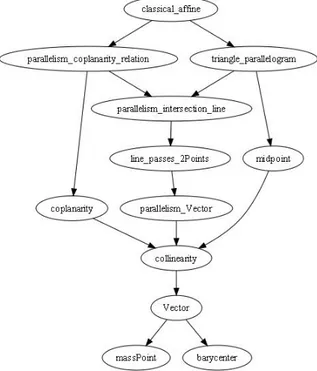
The initial idea of a library in Coq for high-school geometry was proposed by F. Guilhot - a highschool teacher [27][28]. With the aim of illustrating geometry proofs in high-school class room, she developed a library based on educative formation in high-high-school. Her development is organized as in Fig.2.1.
F. Guilhot started her formalization with constructing affine geometry. Algebraic structures and vector spaces are never addressed in school programme. However, the notions of mass point and barycenter are presented in high-school courses, and cal-culations of mass point and barycenter are straightforward and familiar to students. Therefore, F. Guilhot constructed affine space from mass point using the universal space proposed by M.Berger [4]. This construction is explained in [28].
To build up the Euclidean space, the affine structure is enriched with the notion of scalar product of vectors (denoted by −→u · −→v ) which makes it possible to define an Euclidean distance, a measure of angle, etc. Geometric notions are added one by one in the order that they are taught in school.
With about 25000 lines of formalization in 70 files, a large part of the French high-school geometry programme is covered, many geometric notions are formalized and
Figure 2.1: Structure of F. Guilhot’s development
some classical theorems are proved. The detail of formalized geometric notions is as follows.
◦ General affine geometry : basic notions of affine geometry in any dimension are formalized
– Point, mass point, vector, algebraic measure
– Barycenter, midpoint, barycenter properties, gravity center of triangle – Parallel lines, concurrent lines
– Collinearity, co-planarity
◦ Affine geometry of dimension 3 : properties of parallelism and incidence of lines and planes in 3D space are formalized
◦ General Euclidean geometry : the affine structure is enriched with scalar product and the following dependent notions
– orthogonality of vectors and lines
– orthogonal projection of a point on a given line – Euclidean distance
◦ Orthogonality in dimension 3 : orthogonal lines and orthogonal planes are added
◦ Euclidean plane geometry : this is the most important part of high-school geom-etry. It includes
– Notions defined using Euclidean distance : perpendicular bisectors, circles – Coordinates system, orthogonal coordinates system, Cartesian coordinates
system
– Oriented angle of vectors and lines – Trigonometry
– Signed areas of triangles and parallelograms, determinant
◦ Plane transformation : study properties of plane transformation and composed transformations, particularly properties about preservation of length and angle measure
F. Guilhot does not try to provide a system with a minimal number of axioms, nor to provide an automated tool for theorem proving. She does not build up the whole of Euclidean geometry from a fundamental axiomatic system such as the systems of Hilbert or Tarski. An alternative approach is used to arrive at the same geometrical results, where definitions of geometric notions, theorems and geometry reasonings are described as they are taught in high-school. In particular, geometric notions usually are declared as abstract notions, each notion has some companion properties which are stated in the form of axioms to manipulate it. For example, the following is the formalization of the notion of line. An abstract type for lines and an abstract function to construct a line from two points are declared. Two axioms about line properties are introduced, making it possible to manipulate this notion.
V a r i a b l e L i n e : Type . V a r i a b l e l i n e : P o i n t −> P o i n t −> L i n e . Axiom l i n e p e r m u t e : f o r a l l A B : P o i n t , A <> B −> l i n e A B = l i n e B A . Axiom a l i g n e s l i n e : f o r a l l A B C : P o i n t , A <> B −> A <> C −> c o l l i n e a r A B C −> l i n e A B = l i n e A C .
From the pedagogical point of view, defining by properties is a usual manner to de-fine an object in high-school. Students approach geometric notions through properties. This way of defining is appropriate for notions considered to be really primitive notions. But axioms are unnecessary in defining compound notions, which are composed from other ones, and axioms are unnecessary for relations between geometric objects as well. The following formalization is to define orthogonal projection of a point on a line and parallelism relation of lines.
V a r i a b l e o r t h o g o n a l P r o j e c t i o n : P o i n t −>P o i n t −>P o i n t −>P o i n t . Axiom d e f o r t h o g o n a l P r o j e c t i o n 1 : f o r a l l A B C H : P o i n t , A <> B −> o r t h o g o n a l P r o j e c t i o n A B C H −> c o l l i n e a r A B H /\ o r t h o g o n a l ( v e c t o r A B) ( v e c t o r H C ) . Axiom d e f o r t h o g o n a l P r o j e c t i o n 2 : f o r a l l A B C H : P o i n t , A <> B −> c o l l i n e a r A B H −> o r t h o g o n a l ( v e c t o r A B) ( v e c t o r H C) −> o r t h o g o n a l P r o j e c t i o n A B C H . V a r i a b l e p a r a l l e l : L i n e −> L i n e −> Prop . Axiom d e f p a r a l l e l : f o r a l l (A B C D : P o i n t ) ( k : R ) , A <> B −> C <> D −> 1B + ( −1)A = kD + (−k )C −> p a r a l l e l ( l i n e A B) ( l i n e C D ) . Axiom d e f p a r a l l e l 2 : f o r a l l A B C D : P o i n t , A <> B −> C <> D −> p a r a l l e l ( l i n e A B) ( l i n e C D) −> e x i s t s k : R , 1B + ( −1)A = kD + (−k )C .
For orthogonal projections, two axioms are introduced, the first one gets properties from the notion, and the second one inversely gets the corresponding object from the given properties. The first axiom gives us collinearity of the triple of A,B and H, and orthogonality of two vectors−AB and−→ −−→HC if we have that H is the orthogonal projection point of C on line AB. The second asserts that H is the orthogonal projection point of C on line AB if we have collinearity of A,B and H, and orthogonality of −AB and−→ −−→HC.
For the parallelism of lines, two axioms assert that the parallelism of line AB and CD is equivalent to the collinearity of −AB and−→ −−→CD. This collinearity is expressed by −−→
This is a fast way to have a geometry library, which provides notions and properties for students to construct proofs of other theorems. However, this leads to an explosion of the number of axioms and primitive notions. They increase linearly in respect to the number of added notions, with a lot of redundancy. As a result of this, there are about 127 axioms in the library. In our examples, we can define the parallelism of 2 lines AB and CD by collinearity of 2 vectors −AB and−→ −−→CD. Therefore, the two axioms defining parallelism could be dispensed with.
Moreover, the library does not provide functions to construct points, lines and com-pound geometric constructions. They are used in axioms which state their properties without knowing how they are constructed. This makes the library lose the constructive property. This is the case of orthogonal projection in our example. In a constructive view, we can construct the orthogonal projection of C on line A B by getting the in-tersection point of line AB with the line which passes through C and is perpendicular with line AB. Besides, the lack of definitions in the form of functions leads to unusual representations. For instance, orthogonalProjection A B C H expresses the relations of points col ABH ∧ CH ⊥ AB rather than providing a definition of H.
2.3
Reducing axioms and having a constructive library in
a geometric view
In spite of its drawbacks, this library is good from a pedagogical point of view. It matches requirements for a geometric library being used in school. This motivates us to improve this library. Our objective is to find a more compact axiom system, that allows us to rebuild all geometric notions and to prove their properties in this library. To do that, we analyze the library and draw up strategies to reduce its axiom system. We can distinguish geometric notions into geometric constructions and geometric relations. Geometric constructions are geometric objects such as points, lines, circles, angles, altitudes, orthocenters, etc. Geometric relations express relations between these geometric objects, for example the parallelism of lines, the perpendicularity of lines, etc. These relations are essential for the library to manipulate geometric objects and state geometric problems.
For the first category, we continue to divide them into primitive constructions and compound constructions. Primitive constructions are elementary constructions based on ruler and compass. Compound constructions are considered as sequences of elemen-tary constructions. To make our library match dynamic geometry systems, we refer to [31] for the elementary construction list.
As compound constructions are constructed step by step using elementary con-structions, axioms related to them can be eliminated by retracing the combinations of elementary construction. These axioms become theorems that have to be proved. For each compound construction, there are always at least two companion theorems that correspond to axioms used to define this construction in the system of F. Guil-hot showed in the example of the previous section. One of these axioms is to prove properties from the given notion, and the other is to get the corresponding notion from properties. The latter leads to proving the unique existence of a construction with the given properties. This is not always straightforward. The axioms concerning the orthogonal projection of a point C on a line AB in the previous section is an example. We have to prove that there is only a point H such that A, B, and H are collinear and AB ⊥ CH. This allows us to deduce that if H satisfies these properties then H is equal with the orthogonal projection of C on AB which have the same properties.
Reducing axioms related to elementary constructions is more difficult. These con-structions are primitive in the geometric view, but they may be non-primitive in the logical view. For example, lines and circles are primitive constructions. However, we can consider a line as a set of points that are collinear with the 2 given points, a circle as a set of points that have the same distance with respect to the center. Defining notions of this kind depends on the axiom system and the primitive notions from which we build up geometry. Their properties are proved from their definitions. Thus, axioms for these notions can be eliminated.
Once geometric objects are formalized, we have their definition and properties. In-tuitively, it is not difficult to define relations between geometric objects. Thus, reducing the number of axioms used to define these relations comes without much effort.
Besides, there are some notions that come from algebra such as the signed area of a triangle, the trigonometric functions, etc. These notions are usually expressed by algebraic equations, so these equations can help us in definitions.
2.4
Formalization of affine geometry
In this section as well as in some of the next ones about formalization in Coq, we cannot give all the details about our development. We rather focus on some interesting, crucial formalizations of each part. This clarifies the technique we used to eliminate axioms from the library of F. Guilhot.
Figure 2.2: Formalization of Affine Geometry
Figure2.2shows the dependency between files in our formalization for affine geom-etry. The file, namely mass point, contains the formalization of F. Guilhot about the notion with the same name. The following axioms are used for mass point
Axiom I d e m p o t e n c y : nP + mP =(m+n )P .
Axiom C o m m u t a t i v i t y : nP + mQ = mQ + nP .
Axiom A s s o c i a t i v i t y : nP + (mQ + kR ) = ( nP + mQ) + kR . Axiom D e f i n i t i o n o f s c a l a r m u l t i p l i c a t i o n : k ( nP ) = ( k ∗ n )P . Axiom D i s t r i b u t i v i t y k ( nP + mQ) = knP + kmQ .
We use small letters a, b, c, etc. to denote real numbers; capital letters A, B, C, etc. to denote points; pairs consisting of a real number and a point in the form aA to denote mass points.
Here we work with the field of real numbers. It’s familiar with high school students. These axioms were not directly introduced in her formalization. Instead of this, she formalized mass point by making a mapping into an abstract field structure in Coq. Therefore, algebraic properties represented by these axioms is ensured. This formalization enables us to simplify equations of mass points using automated tactics from the Coq library for fields (such as ring_simplify, field_simplify, etc.). It makes calculations easier. The use of mass points is a good approach for computation, and familiar to students.
The file named barycenter is for the notion of barycenter. This notion allows us to create a new point R from the two given mass points nP and mQ in the case n + m 6= 0 such that (n + m)R = nP + mQ and the new point R is called the barycenter of P and Q with the masses n and m respectively. The equality (n + m)R = nP + mQ is rewritten by (n + m)(barycenter np mQ) = nP + mQ. The following axiom is used to define this notion.
Axiom D e f i n i t i o n o f b a r y c e n t e r : ∀ (m n : R e a l ) ( P Q : P o i n t ) m + n 6= 0 → ∃(R : P oint), nP + mQ = (m + n)R
The notion of vector is considered as a sum of 2 mass points with the sum of their masses equals zero. This is represented as follows:
D e f i n i t i o n v e c (A B : P o i n t ) := ( −1)A + 1B .
This definition allows us to convert vectors into mass points so that calculations of vector are translated to the ones of mass points, hence the automatic tactics can be reused. For the detail of this formalization, we refer the reader to publications by F. Guilhot[28][27]. However, we can simply understand that calculations of mass points and vectors are easily realized by some automatic tactics, as in the proofs of the following examples.
The first example states Chasles’ relation for vector−AB +−→ −BC =−→ −→AC.
Lemma t e s t 1 a d d V e c t o r : f o r a l l (A B C : P o i n t ) , v e c A B + v e c B C = v e c A C . P r o o f . i n t r o s . u n f o l d v e c i n ∗ . RingMP . Qed .
By unfolding the definition of vector in the goal, we have to prove that ((−1)A + 1B) + ((−1)B + 1C) = (−1)A + 1C. The tactic RingMP allows us to solve this equality automatically. Simply speaking, the tactic repeatedly performs algebraic transforma-tions to reduce 2 parts of the equality in a normalized form, so that their equality can be decided.
The next example is more complex, it states that if I is the midpoint of BC we have −−→
AB +−→AC = 2−AI. I is represented as the barycenter of B and C with masses 1 and 1→ respectively.
Lemma c a l c u l m i d p o i n t : f o r a l l (A B C I : P o i n t ) , 2 I = 1B + 1C −>
i n t r o s A B C I H . u n f o l d v e c i n ∗ . c u t ( 1 I = ( / 2 ) ( 1B +1C ) ) ( ∗ a s s e r t t h i s f a c t ∗ ) . i n t r o s H0 . r e w r i t e H0 i n ∗ . ( ∗ r e p l a c e 1 I w i t h . . ∗ ) a s s e r t (2 < >0). i n t r o s H1 . FieldMP 2 . . . . Qed .
The proof of this example is similar to the first example. By unfolding the definition of vector, we have to prove that ((−1)A + 1B) + ((−1)A + 1C) = 2((−1)A + 1I). Replacing (1I) with ((/2)(1B + 1C)) in the goal leads us to prove ((−1)A + 1B) + ((−1)A + 1C) = 2((−1)A + ((/2)(1B + 1C))). As in the first example, we have a tactic, namely FieldMP, to solve this equality. A difference between these tactics is that FieldMP is used for equality with fractions of R.
2.4.1 Formalization of vector
Until this point, we preserve the formalization of F. Guilhot. Let’s consider the defini-tion of vector. This nodefini-tion plays a crucial role for our formalizadefini-tion, thus we give the details of formalizing this notion.
The definition of vector allows us to convert vectors into mass points so that cal-culations of vector are translated to the ones of mass points and can be automatically performed. However, it also has some drawbacks. It is a constructor of a vector from two points rather than a definition of vector. Vectors only are a special case of mass point combinations, they do not have a proper type. This leads to ambiguity in the type MassPoint. In particular, with a value v of type MassPoint, we do not know whether v is the representation of a vector or not. Furthermore, the lack of a clean type forces us to use vectors in the form of−AB, we do not have −−→ →v without precise points. This leads to difficulties when defining geometric notions where vectors are used as arguments in the definition.
Data structure for vector
We aim at providing a new type for vector so that automatic calculations are in-herited. In fact, a value of mass point v is a vector if there are 2 points A and B such that v can be expressed by v = (−1)A + 1B. Our approach uses a sub-type of mass point for vector.
First, we define a function, namely isVector, of type M assP oint → P rop that takes a mass point value and returns true if v is a representation of a vector. In other words, there are two points A, B such that v = (−1)A + 1B. This function is then used as a filter in the following definition of vector.
D e f i n i t i o n i s V e c t o r ( v : M a s s P o i n t ): = e x i s t s A , B : P o i n t , v = ( −1)A + 1B .
R e c o r d V e c t o r : Type :=
v e c C o n s { mpOf : M a s s P o i n t ; p r o o f : i s V e c t o r mpOf } .
Vector is defined by the record containing two fields. The first one mpOf is a value of mass point. The second is a proof showing that the first is a representation of a vector. We use the pair (mpOf, proof) to denote vector. Note that we use here the notion of dependent type in Coq where the type of some argument to a function depends on the value of other arguments. Indeed, the element proof has the type of isVector mpOf (essentially ∃AB :Point, mpOf = (-1)A + 1B ), hence its type depends on the value of mpOf.
Constructor for vector
The first functions that we have to consider after having created the type Vector are constructors. For a vector, we only have one constructor in the form of vector A B. Defining this constructor is simple by the mass point value (−1)A + 1B and the trivial proof p showing this value is a representation of a vector. In particular, there exist two points A’ and B’ such that (−1)A + 1B = (−1)A0+ 1B0.
Definition of operators
We now define algebraic operators of vectors. It is easy to find that we can define these operators by using their correspondence in mass point. In particular, we define the addition operator of two vectors by constructing the vector addition from the sum of mass point values of these vectors.
D e f i n i t i o n a d d V e c t ( v1 v2 : V e c t o r ) :=
match v1 , v2 w i t h ( mpOf1 , p r o o f m p O f 1 ) , ( mpOf2 , p r o o f m p O f 2 ) => ( ( mpOf1 + mpOf2 ) , ( s u m V e c s i s V e c mpOf1 mpOf2 ) )
end .
This definition is interpreted as follows: v1 and v2 have the type Vector, suppose that they are represented by records (mpOf1,proof mpOf1) and ( mpOf2, proof mpOf2). We then construct a record of type Vector that takes (mpOf 1 + mpOf 2) as the mass point value and consider it as the vector addition. The second element of this vector
is a proof showing that (mpOf 1 + mpOf 2) is a representation of vector. This proof is provided by the function sumVecs isVec constructed using isVector as follows
Lemma s u m V e c s i s V e c :
f o r a l l ( v a l u e 1 v a l u e 2 : M a s s P o i n t ) , i s V e c t o r v a l u e 1 −> i s V e c t o r v a l u e 2 −> i s V e c t o r ( v a l u e 1 + v a l u e 2 ) .
Once this lemma is proved, its application with arguments mpOf1 and mpOf2 (sumVecs isVec mpOf1 mpOf2 ) gives us an object with the type isVector ( mpOf1 + mpOf2). Thus we can use this as the second element of the vector resulting from the addition.
...Begin of Technical Details... 1.
To prove this lemma, we first introduce hypotheses and destruct the hypotheses isVector value1 and isVector value2 to have 4 points A, B, C and D such that
value1 = (−1)A + 1B and value2 = (−1)C + 1D. P r o o f . i n t r o s v a l u e 1 v a l u e 2 H0 H1 . d e s t r u c t H0 a s [ A [ B H0 ] ] . d e s t r u c t H0 a s [ C [ D H1 ] ] . H0 : v a l u e 1 = ( −1)A+1B H1 : v a l u e 2 = ( −1)C+1D ( 1 / 1 ) i s V e c t o r ( v a l u e 1 + v a l u e 2 )
By unfolding isVector in the goal and rewriting value1 and value2 by their represen-tation of points, we have to prove ∃A0 B0, (−1)A0+ 1B0 = (−1)A + 1B + (−1)C + 1D. Observe that, if we choose A0 = A, (1B0) can be calculated by (−1)A + 1B0 = (−1)A + 1B + (−1)C + 1D, hence 1B0 = 1B + (−1)C + 1D.
We recall that with 2 mass points aA and bB where a+b 6= 0, we can construct their barycenter such that ∀(ab : R)(AB : P oint), a + b 6= 0 → (a + b)(barycenter aA bB) = aA + bB.
The sum of masses in the right hand side of the above equality differs from 0. Therefore, it is evident that we can construct B’ by using the barycenter. The con-struction of B’ is as follows : 1B0 = 1B + (−1)C + 1D ⇒ 1B0 = (−1)C + (1B + 1D) ⇒ 1B0 = (−1)C + (2(barycenter1B1D))(apply the property of barycenter with 1B
and 1D) ⇒ 1B0 = 1(barycenter(−1)C(2(barycenter1B1D))) (apply the property of barycenter with (-1)C and 2(barycenter 1B 1D)).
The proof of existence of A’and B’is performed by respectively assigning A and (barycenter (-1)C (2(barycenter 1B 1D))) to them. These assignment are performed in Coq by tactic exists as follows
P r o o f . . . r e w r i t e H0 , H1 . u n f o l d i s V e c t o r . e x i s t s A . e x i s t s ( b a r y c e n t e r (( −1)C) ( 2 ( b a r y c e n t e r ( 1B) ( 1D ) ) ) ) . H0 : v a l u e 1 = ( −1)A+1B H1 : v a l u e 2 = ( −1)C+1D ( 1 / 1 ) ( −1)A+1( b a r y c e n t e r ( −1)C ( 2 ( b a r y c e n t e r 1B 1D))=( −1)A+1B+(−1)C+1D
To prove this new goal, we use the property of barycenter in inverse direction with the above construction of B’. We make occurrences of barycenter disappear by repeatedly replacing (a + b)(barycenter aA bB) with aA + bB. The proof obligation becomes (−1)A + ((−1)C + (1B + 1D)) = (−1)A + 1B + (−1)C + 1D. This is solved by the tactic RingMP mentioned above.
P r o o f . . .
r e p e a t r e w r i t e b a r y c e n t e r p r o p ; auto . Ring MP .
Qed .
...End of Technical Details... Similarly, we define the multiplication of vector.
Lemma m u l t V e c i s V e c : f o r a l l ( k : R) ( mpOf : PP ) , i s V e c t o r mpOf −> i s V e c t o r ( mult PP k mpOf ) . D e f i n i t i o n m u l t V e c t ( k : R) ( v1 : V e c t o r ) := match v1 w i t h v e c C o n s mpOf p r o o f m p O f => v e c C o n s ( m u l t V e c i s V e c k mpOf ) end .
Tactic to translate calculations of vectors
By these operator definitions, calculations of vectors are essentially performed with their mass point value. However, to be able to reuse automatic calculations of mass
points, we need to translate equalities of vector in the proof context to equalities of mass points. The following tactic is designed to do this in Coq:
L t a c t r a n s f V e c t o r M a s s P o i n t := ( ∗ s t e p 1 : c o n v e r t t o s t r u c t u r e ∗ ) r e p e a t match g o a l w i t h | |− c o n t e x t [ v e c t o r ] => u n f o l d v e c t o r | |− c o n t e x t [ a d d V e c t ] => u n f o l d a d d V e c t | |− c o n t e x t [ m u l t V e c t ]=> u n f o l d m u l t V e c t | H : c o n t e x t [ v e c t o r ] |− => u n f o l d v e c t o r i n H | H : c o n t e x t [ a d d V e c t ] |− => u n f o l d a d d V e c t i n H | H : c o n t e x t [ m u l t V e c t ] | − => u n f o l d m u l t V e c t i n H end ; ( ∗ s t e p 2 : t r a n s l a t e s t r u c t u r e t o mass p o i n t ∗ ) r e p e a t match g o a l w i t h | |− v e c C o n s ? a = v e c C o n s ? b => r e w r i t e <− M a s s P o i n t V e c t o r e q u i v ; s i m p l | H : v e c C o n s ? a = v e c C o n s ? b |− => r e w r i t e <−M a s s P o i n t V e c t o r e q u i v i n H ; s i m p l i n H | => i d t a c end ) .
The tactic is performed in 2 steps. In the first step (corresponding to the first repeat loop), we convert all terms of type Vector into their structure. We only have three functions that return an element of type Vector and these are converted as follows
◦ The constructor of vector vector A B is converted to ((-1)A+1B, )
◦ The addition function add Vect u v is converted to (mpOf u + mpOf v, )
◦ The multiplication function mult Vect k v is converted to (k (mpOf v), )
These conversions are performed repeatedly. As a result, an equality of two terms of type Vector is replaced by an equality of calculated structures that represent these terms. For example, −→w = k−→u + l−→v is converted to (mpOf w, ) = ((k(mpOf u) + l(mpOf v)), ).
In the second step (corresponding to the second repeat loop), the equalities of structure are translated to ones of their corresponding mass point by using the following equivalence
M a s s P o i n t V e c t o r e q u i v : f o r a l l v1 v2 : V e c t o r , mpOf v1 = mpOf v2 <−> v1 = v2
In Coq the equality of two objects of type Record is only ensured by equal-ity of all their components mpOf v1 = mpOf v2 ∧ proof v1 = proof v2 ↔ (mpOf v1, proof v1) = (mpOf v2, proof v2) ↔ v1 = v2. So, to prove this lemma, we have to use the irrelevant proof in Coq, which shows that all proofs of a property are equivalent.
Axiom p r o o f i r r e l e v a n c e : f o r a l l (P : Prop ) ( p1 p2 : P ) , p1 = p2 .
Using this equivalence, the tactic finds equalities of vector structure in the proof context, and repeatedly replaces them by equalities of mass points. For example, after doing this step, −→w = k−→u + l−→v is replaced by mpOf w = (k(mpOf u) + l(mpOf v).
Using this tactic allows us to easily prove algebraic properties of vector. Indeed, we only need to use the tactic transf Vector MassPoint to get equalities of mass point and the automatic tactics on mass points to perform calculations. For example, the proof of distributivity for vectors is short as follows:
Lemma m u l t V e c t a d d V e c t d i s t r i b u t i v e : f o r a l l ( r : R) ( v1 v2 : V e c t o r ) , m u l t V e c t r ( a d d V e c t v1 v2 ) = a d d V e c t ( m u l t V e c t r v1 ) ( m u l t V e c t r v2 ) . P r o o f . i n t r o s . d e s t r u c t v1 ; d e s t r u c t v2 . ( ∗ t o r e p r e s e n t v e c t o r by p o i n t s ∗ ) t r a n s f V e c t o r M a s s P o i n t . RingMP . Qed .
The last properties of vector that we would like to present concern creating new point as barycenters. In the proofs of the lemma sumVecs isVec, we can see somewhat the relation between them. Indeed, we saw the analysis to find out B’ such that (−1)A + 1B0 = (−1)A + 1B + (−1)C + 1D. This analysis leads us to construct B’ using barycenter B0 = (barycenter(−1)C(2(barycenter 1B 1D))). In other words, we can construct B’ such that −−→AB0=−AB +−→ −−→CD.
In a generalized form of this, a question is that, with any point M and algebraic combination of vectors, if we can construct a point N such that −−→M N equals this com-bination. The answer is yes by constructing N with the help of the barycenter function using a similar analysis. The following lemmas state the existence of such an N for some combinations. Note that we use operator addition and multiplication instead of add Vect and mult Vect
Lemma e x i s t e n c e m u l t V e c t R e p r e s e n t a t i v e : f o r a l l (M A B : P o i n t ) ( k : R ) ,
{N | −−→M N = k −AB } .−→
f o r a l l (M A B C D : P o i n t ) , {N | −−→M N = −AB +−→ −−→CD } .
Lemma e x i s t e n c e l i n e a r C o m b V e c t R e p r e s e n t a t i v e : f o r a l l (A B C D M : P o i n t ) ( k1 k2 : R ) ,
{N | −−→M N = k1 −AB + k2−→ −−→CD } .
Note that the statements of the lemmas use constructive existence. Roughly speak-ing, {x:A|P x} is a type and an instance of this type gives us an object satisfying the property P. This differs from ∃x, P x that renders a proof. The first form is stronger than the second form. Indeed, if we can construct an object satisfying the property P, we can obviously prove the existence of an object satisfying the property P by using the newly constructed object.
As a result, proofs of these lemmas have to be performed in a constructive way. It means that we have to give a construction for N satisfying the requirements of the lemmas. For example, in the lemma existence multVectRepresentative, we need to construct N such that −−→M N = k−AB. We have (−1)M + 1N = k((−1)A + 1B) →−→ 1N = (−k)A + kB + 1M → 1N = 1(barycenter (−k)A(k + 1)(barycenter kB 1M )), hence N = (barycenter (−k)A(k + 1)(barycenter kB 1M )). This assignment of N allows us to readily prove that −−→M N = k−AB by calculations of mass point.−→
We will later see the role of these properties in constructing Cartesian coordinate systems, defining midpoint, and defining some plane transformations.
2.4.2 Formalization of line
The notion of vector allows us to formalize the other notions in affine geometry (see Fig. 2.2). The following is a short presentation about it.
◦ The middle of two points and the gravity center of a triangle are defined using barycenters. In particular, the midpoint I of A and B is defined as the barycenter of the mass points 1A and 1B,
midpoint A B := barycenter 1A 1B.
The gravity center G of triangle ABC is defined by barycenter of 1A 1B and 1C,
gravity A B C := barycenter 1A 2(barycenter 1B 1C).
We can prove its properties such as: G ∈ CI and −→AG = 23−AI when I is the→ midpoint of BC, 3 medians of triangle intersect at G, etc.
◦ The parallelism of vectors is defined by collinearity. The definition is as follows v1 k v2 := v2 6=−→0 ∧ ∃k : R, k 6= 0 ∧−v1 = k→ −→v2.
◦ The collinearity of three points is defined by using collinearity of vectors as follows
col A B C := A = B ∨ ∃k : R,−→AC = k−AB.−→
◦ Coplanarity is defined by showing that a vector is a combination of other vectors. In particular, coplanarity of A, B, C, and D is defined by
coplanar A B C D := ∃(k1 k2 : R),−AD = k1−→ −AB + k2−→ −→AC.
◦ Intersection of lines is defined by the existence of a common point. Relations between intersection, coplanarity and parallelism are introduced, for example
intersect (line AB)(line CD) → coplanar A B C D,
¬parallel (line AB)(line CD) → intersect (line AB)(line CD)∨¬coplanar A B C D.
Notions in affine geometry are formalized and their properties are also proved. We now pay attention to the notions of parallelism of lines that are the heart of affine geometry. We present our formalization by comparing it with the one realized in the library of F. Guilhot, this allows readers to see the advantages of our approach and how we eliminate axioms. F. Guilhot considered lines as an abstract object, there is a function to construct a line from two points and axioms allowing to manipulate this type of line. V a r i a b l e l i n e : P o i n t −> P o i n t −> L i n e . Axiom l i n e p e r m u t e : f o r a l l A B : P o i n t , A <> B −> l i n e A B = l i n e B A . Axiom c o l i n e a r l i n e : f o r a l l A B C : P o i n t , A <> B −> A <> C −> c o l i n e a r A B C −> l i n e A B = l i n e A C .
In a Coq view, these axioms are strong because they state equalities of objects. Ev-idently, properties are preserved from one to the other. Therefore, using these axiom make the system weaker. Moreover, this formalization only provides only one construc-tion of line using different points. Two other types of line, line passing through a point and perpendicular with a given line (denoted tline) and line passes through a point and parallel with a given line (denoted pline), were not approached in the library of F. Guilhot. Adding these would lead to auxiliary axioms. Besides, the lack of common structure that represents line raises difficulties in defining relations of lines, for example, parallelism of two lines have to be precisely defined for each type of line.
To fill these gaps, we need to devise a common data structure for all types of line. We then define operators and relations concerning lines for this structure. Line constructors corresponding the types of line are also introduced. Finally, properties of line is verified with this formalization.
Data structure for line
We chose to represent lines with a root point and a non zero direction vector. In Coq, this is expressed by a record with three elements, where the first is a point, the second is a vector, and the last is the proof that the vector is non zero. Once again, the structure Record with a dependent type is used.
R e c o r d L i n e : Type := l i n e C o n s
{ r o o t O f : P o i n t ; v e c O f : V e c t o r ; p r o o f N o n Z e r o : i s N o n Z e r o V e c v e c O f } .
Definition of operators and relations
Equality : As done with vector, the first notion we need to define is the equality of lines. We observe that, in the case that two lines have the same root point, they are equal if the two direction vectors are collinear. In the other case, two lines are equal if the vector composed by the two root points and the two direction vectors are collinear. The equality of two lines a = (A, −→u ) and b = (B, −→v ) is defined by
a == b := − →u k −→v if A = B − →u k −→v k−AB−→ if A 6= B
In Coq this is expressed by
D e f i n i t i o n l i n e E q u a l : ( a b : L i n e ) := match a , b w i t h (A , −→u ) , (B , −→v )
=> (A = B → −→u k −→v ) ∧ (A 6= B → (−AB k −−→ →u ∧ −→u k −→v ) .
We here remark that notions of “a==b” and “a=b” are different in Coq. The first expresses equivalence of lines, it is mapped to semantic equality of lines in geometry. It is coarser than the second notion which expresses equality of line at the level of data structures. This distinction will be clarified in the discussion section at the end of this chapter.
Parallelism : The representation of lines using a direction vector makes it easier to define the parallelism of lines. In fact, the parallelism of lines is defined by the parallelism of their direction vector. The parallelism of vectors is already defined. With a = (A, −→u ) and b = (B, −→v ), we define a k b := −→u k −→v .
A point lying on a line: a point lies on a line if and only if the vector, composed by this point with the root point of the line, and the direction vector are collinear. With a = (A, −→u ) and a point M, we define M ∈ a :=−−→AM k −→u .
Definition of constructors
In this session, we present only 2 types of line: line with 2 points and parallel line. The remaining kind (perpendicular) is only formalized in Euclidean geometry where we have the notion of perpendicularity.
A line passing through two different points A and B is constructed by the root point A and the direction vector −AB. In the degenerate case where A and B coincide,−→
we return an arbitrary value for this line. The principle of excluded middle is used to determine cases of A and B. This is represented through a function AB decidable that gives us A=B or A<>B.
Lemma i s N o n Z e r o V e c C o n d i t i o n : f o r a l l A B : P o i n t , A<>B −>i s N o n Z e r o V e c ( v e c t o r A B ) . P a r a m e t e r a r b i t r a r y L i n e : L i n e . D e f i n i t i o n l i n e (A B : P o i n t ) := match ( @ A B d e c i d a b l e (A = B ) ) w i t h | l e f t H => a r b i t r a r y L i n e | r i g h t H => l i n e C o n s A ( v e c t o r A B) ( i s N o n Z e r o V e c C o n d i t i o n (A:=A ) ( B:=B) H) end .
The chosen structure representing line emphasizes the role of vectors. The role of the second point in formalization of F. Guilhot is blurred. Using the direction vector makes it easier to formalize the line passing through a point and perpendicular with a given line (denoted tline) and the line passes through a point and parallel with a given line (denoted pline). Indeed, if we want to construct a line passing a point A and parallel with a given line, we can always use A as the root point of this line. As a result, defining a line leads to constructing its direction vector.
For the pline lp passing a point A and is parallel with a given line a = (B, −→u , prf ), it
is easy to find that −→u can be used as the direction vector of lp. The element prf that is
a proof of −→u 6=−→0 is also reused. Thus, the parallel line is defined by lp := (A, −→u , prf ).
D e f i n i t i o n l i n e P (A : P o i n t ) ( a : L i n e ) := match a w i t h l i n e C o n s B u p r f
=> l i n e C o n s A u p r f end .
Verification of properties
Our formalization allows us to verify properties of lines. The first ones that we want to cite here are the properties stated as axioms in the library of F. Guilhot.
Lemma a l i g n p e r m u t e : f o r a l l A B : P o i n t , A <> B −> l i n e A B == l i n e B A .
Lemma a l i g n l i n e : f o r a l l A B C : P o i n t , A <> B −> A <> C −>
c o l A B C −> l i n e A B == l i n e A C .
The first lemma can be proved easily. For the second one, we start with the hy-potheses A 6= B and A 6= C we have that −AB 6=−→ −→0 and −→AC 6=−→0 . By the definition of line −AB and−→ −→AC are direction vectors of the line AB and the line AC respectively. By the definition of collinearity (col A B C) we have that−AB and−→ −→AC are collinear. Thus line AB == line AC by the definition of equality of lines for the case where lines have the same root point.
Other properties of lines are also proved. They include: the transitivity of par-allelism ∀a b c, k b ∧ b k c → a k c; properties of parallel lines such as ∀(A : point)(l : Line), pline(A l) ↔ A ∈ l ∧ pline(A l) k l; properties related to ly-ing on a line such as ∀A B, A 6= B ∧ A ∈ a ∧ B ∈ a → line A B == a and ∀A B C, A 6= B ∧ C ∈ line A B → col A B C.
2.5
Formalization of Euclidean geometry
In affine geometry, there is no way to talk about distances, orthogonality and angles. Euclidean geometry is built from affine geometry by adding axioms about the notion of scalar product (denoted by −→u · −→v ). This is also called dot product or inner product. The axioms of scalar products are introduced in Coq as follows
V a r i a b l e s c a l a r P r o d u c t : V e c t o r −> V e c t o r −> R . Axiom s c a l a r P r o d u c t p o s i t i v e V e c t o r : f o r a l l v : V e c t o r , s c a l a r P r o d u c t v v >= 0 . Axiom s c a l a r P r o d u c t n o n d e g e n e r a t e V e c t o r : f o r a l l v : V e c t o r , s c a l a r P r o d u c t v v = 0 −> v = Z e r o V e c t . Axiom s c a l a r P r o d u c t s y m : f o r a l l u v : V e c t o r , s c a l a r P r o d u c t u v = s c a l a r P r o d u c t v u . Axiom s c a l a r P r o d u c t a d d V e c t l : f o r a l l v1 v2 v3 : V e c t o r , s c a l a r P r o d u c t ( a d d V e c t v1 v2 ) v3 = s c a l a r P r o d u c t v1 v3 + s c a l a r P r o d u c t v2 v3 . Axiom s c a l a r P r o d u c t m u l t V e c t l : f o r a l l ( k : R ) ( u v : V e c t o r ) , s c a l a r P r o d u c t ( m u l t V e c t k u ) v = k ∗ s c a l a r P r o d u c t u v .
Where R is the type for real numbers. The scalar product in turn is used to define the followings entities
◦ Length: the length of a vector −→v is defined to be |−→v | = √−→
v · −→v . In Coq, we have
D e f i n i t i o n m a g n i t u d e ( v : V e c t o r ) := s q r t ( s c a l a r P r o d u c t ( v ) ( v ) ) .
◦ Normalization: Given a nonzero vector −→v . Normalization of −→v is a vector of unit length that points in the same direction as −→v . We have −→v = |−−→→vv |. In Coq we
have to use a function, namely scalarVV decidable vec1, to decide that −→v · −→v = 0 or −→v · −→v 6= 0, these correspond to the case whether −→v =−→0 or not.
D e f i n i t i o n u n i t V e c t o r r e p r e s e n t a t i o n ( v e c 1 : V e c t o r ) := match ( s c a l a r V V d e c i d a b l e v e c 1 ) w i t h
| l e f t H => a r b i t r a r y U n i t V e c t
| r i g h t H => m u l t V e c t ( / ( s q r t ( s c a l a r P r o d u c t v e c 1 v e c 1 ) ) ) v e c 1 end .
◦ Distance between points: the distance between two points is the length of the vector composed by these points, denoted by |AB|
D e f i n i t i o n d i s t a n c e (A B : P o i n t ) :=
s q r t ( s c a l a r P r o d u c t ( v e c t o r A B) ( v e c t o r A B ) ) .
◦ Orthogonality: Given 2 vectors −→u and −→v , we say that they are orthogonal if and only if their scalar product is equal to 0. In Coq, we have
D e f i n i t i o n o r t h o g o n a l ( v e c 1 v e c 2 : V e c t o r ) := s c a l a r P r o d u c t v e c 1 v e c 2 = 0 .
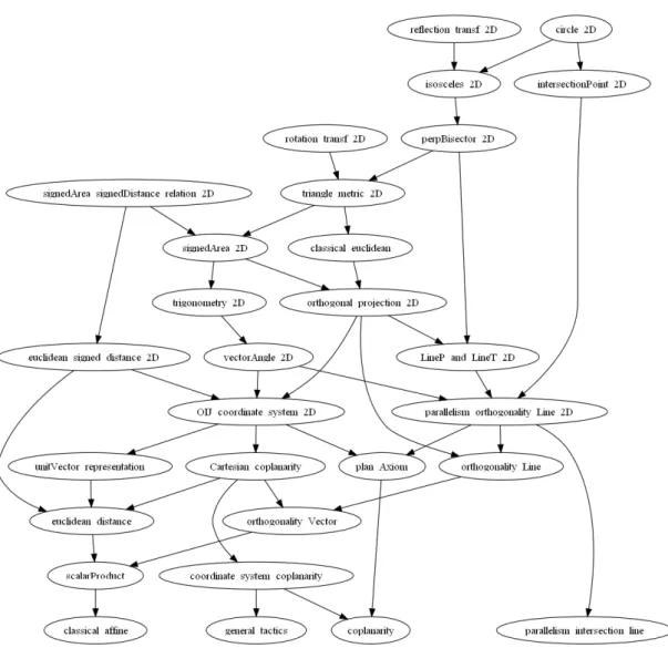
Figure 2.3: Formalization of Plane Geometry
Other notions of Euclidean geometry are introduced one by one into the library. Our formalization is illustrated in Fig.2.3. We now focus on the formalization of some
notion in plane geometry where the following axioms are used. These axioms assert the existence of 3 non-collinear points and their co-planarity with any fourth point.
◦ Axiom about existence of 3 not aligned points: there are 3 different and non-aligned points O, O1 and O2.
◦ Axiom about coplanarity: for any 4 points A, B, C and D in the plane, we always have that A, B and C are collinear or −AD is linear combination of−→ −AB and−→ −→AC.
In fact, formalization of plane geometry is compatible with any plane defined by 3 non-collinear points. However, to make less complex statements and proofs in our library, we suppose the existence of 3 non-collinear points O, O1 and O2, and consider properties
in this plane.
2.5.1 Cartesian coordinate system
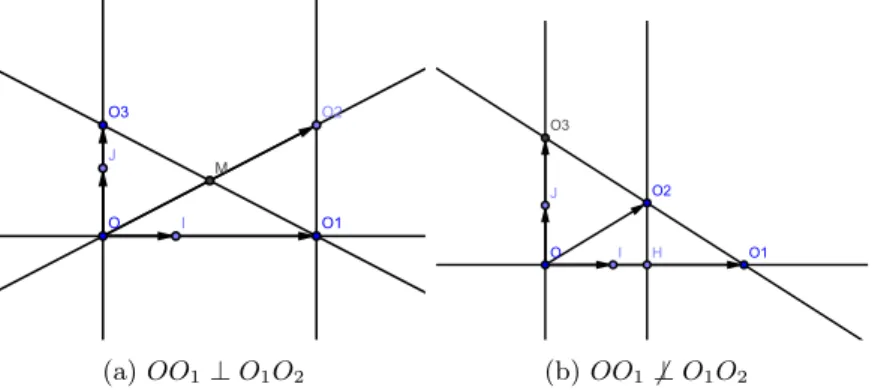
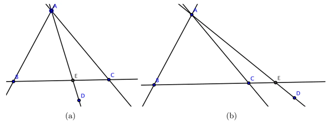
The first notion whose formalization we want to present is a Cartesian coordinates system. This notion not only plays a crucial role in formalizations of many notions such as perpendicular line, trigonometry functions, signed area, etc, but also is a fundamental notion of algebraic geometry. A Cartesian coordinates system is represented by three non-collinear points that form two orthonormal vectors. In other words, they are two orthogonal vectors and both of them have unit length. The notions of orthogonality, distance, unit length that have been presented allow us to formalize this coordinate system. We present how to construct I, J , such that O, I and J form a Cartesian coordinate system, from three arbitrary non-collinear points O, O1 and O2. We now
(a) OO1⊥ O1O2 (b) OO16⊥ O1O2
Figure 2.4: Constructing a Cartesian coordinate system
have to construct I and J satisfying−→OI ·−→OJ = 0 (or−→OI ⊥−→OJ ), |OI| = 1 and |OJ | = 1. Let’s consider the two configurations of O, O1, O2 in Fig.2.4.
For the first case −−→OO1 ⊥
−−−→
O1O2, we construct O3 such that
−−→ OO3 = −−−→ O1O2. From the hypothesis −−→OO1 ⊥ −−−→ O1O2 we have −−→ OO3 ⊥ −−→ OO1.
For the second case−−→OO1 6⊥
−−−→
O1O2, Suppose that H is the orthogonal projection of
O2 on OO1. O3 is constructed from O1, O2 by −−−→ O2O3= −−→ HO −−→ HO1 −−−→ O2O1= −−→ O2O · −−→ OO1 −−−→ O2O1· −−→ OO1 −−−→ O2O1
It’s easy to find that this construction give us
−−−→ O1H −−→ O1O = −−−→ O1O2 −−−→ O1O3 . This leads to−−→OO3k −−→ HO2. As −−→O2H ⊥ −−→ OO1, we get −−→ OO3 ⊥ −−→ OO1.
For the both case, O 6= O1and O 6= O3are easily proved. This allows us to construct
I and J by −→OI = |OO1 1|× −−→ OO1 and −→ OJ = |OO1 3|× −−→ OO3 respectively. −→ OI is a unit vector of −−→OO1, therefore |OI| = 1. −→
OJ is a unit vector of −−→OO3, therefore |OJ | = 1. On the
other hand, we have −→OI ⊥ −→OJ by −−→OO1 ⊥
−−→
OO3. This Cartesian coordinate system is
well formed.
Using this idea, the formalization in Coq is as follows:
D e f i n i t i o n O3:= match twocaseofOO1O2 w i t h | l e f t => p r o j 1 s i g ( @ e x i s t e n c e m u l t V e c t R e p r e s e n t a t i v e O O1 O2 1 ) | r i g h t => p r o j 1 s i g ( @ e x i s t e n c e m u l t V e c t R e p r e s e n t a t i v e O2 O2 O1 −−→ O2O·−−→OO1 −−−→ O2O1·−−→OO1) end . D e f i n i t i o n I := p r o j 1 s i g ( @ e x i s t e n c e m u l t V e c t R e p r e s e n t a t i v e O O O1 |OO1|1 ) . D e f i n i t i o n J := p r o j 1 s i g ( @ e x i s t e n c e m u l t V e c t R e p r e s e n t a t i v e O O O3 |OO3|1 ) . D e f i n i t i o n o r t h o n o r m a l c d n S y s (O I J : P o i n t ) := −→ OI ·−→OJ = 0 ∧−→OI ·−→OI = 1 ∧−→OJ ·−→OJ = 1
Where, the function twocaseofOO1O2 is to decider whether−−→OO1 ·−−−→O1O2 = 0 or not. The application of @existence multVectRepresentative A B C k is to construct a point D such that −AD = k−→ −BC as mentioned in page−→ 21.
To verify if O, I and J form a Cartesian coordinate system, we have to prove that orthonormal cdnSys O I J . We here focus only in the proof of −→OI ·−→OJ = 0 for the case −−→OO1 ·−−−→O1O2 6= 0. By construction of I and J, −→OI and −→OJ are normalizations of −−→
OO1 and
−−→
OO3. This leads us to prove that
−−→ OO1 ·
−−→
OO3 = 0. The proof of this fact
is different with our analysis in constructing O3 where we use this reasoning −−−→ O1H −−→ O1O = −−−→ O1O2 −−−→ O1O3 ⇒ −−→OO3 k −−→ HO2 ⇒ −−→ OO3 ⊥ −−→
OO1. Our proof in Coq is realized by calculations of
scalar products as follows.
...Begin of Technical Details... 2.
We recall some axioms about scalar product mentioned in page26. We have: scalarP roduct sym : ∀uv, −→u · −→v = −→v · −→u ,