Monocular Visual Shape Tracking and Servoing for Isometrically Deforming Objects

(1)

HAL Id: hal-03144911

https://hal.uca.fr/hal-03144911

Submitted on 17 Feb 2021

HAL is a multi-disciplinary open access

archive for the deposit and dissemination of

sci-entific research documents, whether they are

pub-lished or not. The documents may come from

teaching and research institutions in France or

abroad, or from public or private research centers.

L’archive ouverte pluridisciplinaire HAL, est

destinée au dépôt et à la diffusion de documents

scientifiques de niveau recherche, publiés ou non,

émanant des établissements d’enseignement et de

recherche français ou étrangers, des laboratoires

publics ou privés.

Monocular Visual Shape Tracking and Servoing for

Isometrically Deforming Objects

Miguel Aranda, Juan Antonio Corrales Ramon, Youcef Mezouar, Adrien

Bartoli, Erol Ozgur

To cite this version:

Miguel Aranda, Juan Antonio Corrales Ramon, Youcef Mezouar, Adrien Bartoli, Erol Ozgur.

Monoc-ular Visual Shape Tracking and Servoing for Isometrically Deforming Objects. 2020 IEEE/RSJ

Inter-national Conference on Intelligent Robots and Systems (IROS), Oct 2020, Las Vegas, United States.

pp.7542-7549, �10.1109/IROS45743.2020.9341646�. �hal-03144911�

(2)

Monocular Visual Shape Tracking and Servoing

for Isometrically Deforming Objects

Miguel Aranda, Juan Antonio Corrales Ramon, Youcef Mezouar, Adrien Bartoli and Erol Özgür

Abstract— We address the monocular visual shape servoing problem. This pushes the challenging visual servoing problem one step further from rigid object manipulation towards de-formable object manipulation. Explicitly, it implies deforming the object towards a desired shape in 3D space by robots using monocular 2D vision. We specifically concentrate on a scheme capable of controlling large isometric deformations. Two important open subproblems arise for implementing such a scheme. (P1) Since it is concerned with large deforma-tions, perception requires tracking the deformable object’s 3D shape from monocular 2D images which is a severely underconstrained problem. (P2) Since rigid robots have fewer degrees of freedom than a deformable object, the shape control becomes underactuated. We propose a template-based shape servoing scheme in which we solve these two problems. The template allows us to both infer the object’s shape using an improved Shape-from-Template algorithm and steer the object’s deformation by means of the robots’ movements. We validate the scheme via simulations and real experiments.

I. INTRODUCTION

Problem and challenges. A particular problem that has

entered into robotic terminology recently is visual shape

servoing [1]. It differs from classical visual servoing [2] by

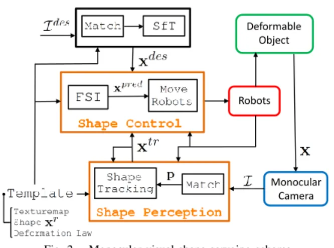
using vision to control not only the robot’s pose but also the object’s deformation. Monocular visual shape servoing requires to solve two significant open problems: (P1) shape perception and (P2) shape control [3]. Firstly, shape control is challenging because it requires to regulate the infinite degrees of freedom of the object’s shape with a finite number of actuation points. Secondly, shape perception is challenging because it requires tracking the deformable object’s 3D shape from 2D images. A suitably accurate, robust and fast estima-tion of the 3D shape is a key ingredient to facilitate visual shape servoing, especially for handling large deformations. Here, we propose a novel monocular visual shape servoing scheme in which we solve the two problems by using the object’s template. The template contains information about the object’s geometry, appearance and deformation behavior. We consider the specific case of isometric deformation, which preserves distances. We model it using a distance-preserving deformation law. The proposed scheme shown in figure 1 is capable of handling large isometric deformations.

The authors are with Université Clermont Auvergne, CNRS, SIGMA Clermont, Institut Pascal, F-63000 Clermont-Ferrand, France. Correspond-ing author: Miguel Aranda, email:miguel.aranda@sigma-clermont.fr. This work was supported by projects COMMANDIA (SOE2/P1/F0638) which is cofinanced by Interreg Sudoe Programme (European Regional Development Fund), and SOFTMANBOT, which received funding from the European Union’s Horizon 2020 research and innovation programme under grant agreement No 869855.

Shape perception. We present an algorithm based on

Shape-from-Template (SfT) [4], [5]. This is a suitable choice because for isometric deformations, SfT can provably find the true shape [4]. We start from Particle-SfT [6], an al-gorithm that models the object as a system of particles. A robotic manipulation task poses specific challenges, such as computation time constraints and occlusions. Our algorithm improves Particle-SfT and can deal with these challenges.

Shape control.Our solution for shape control takes as

in-put the current shape and a desired shape. It uses the template to compute a feasible interpolated 3D shape between the two shapes. It then determines end-effector motions that move the object towards the interpolated 3D shape.

Shape control Shape perception SfT Current image Desired image Desired 3D shape Current 3D shape

Fig. 1. Overview of the proposed visual shape servoing scheme.

Contribution.Our proposed scheme servos explicitly the

full shape of an object in 3D space using only a monocular camera. Existing works for monocular shape servoing in-stead control a reduced representation of the object encoded by low-dimensional image-based features [1], [7]–[12]. In addition, they consider moderate deformations. In contrast, our scheme both tracks and servos the 3D shape in full and across large deformations, using the template. Its servo loop works with just a handful of image points as feedback which makes it robust to occlusions. Furthermore, the template does not need precise identification of the object’s mechanical parameters. Moreover the shape tracking and servoing com-putations of our scheme run fast.

The scheme we propose can be used in industrial sce-narios where isometrically deforming objects (e.g., sheets of paper/cardboard or carbon fiber, fabrics, shoe parts) are commonplace. It only needs a monocular camera which is the de-facto sensor in numerous applications due to its

(3)

many advantages (light-weight, small, cheap). We present results from simulations and real experiments that validate the usefulness of our scheme and illustrate its performance.

II. RELATEDWORK

A. Deformable object tracking under robotic manipulation We focus on works where robots interact with the tracked object. The works [13]–[16] use an RGBD camera to track textureless deformable objects. Particularly, [16] focused on satisfying the requisites of a shape servoing task: principally, fast computation and robustness to occlusion (caused by the robots and the object). Indeed, occlusion is a major factor that makes the tracking problem hard; an illustration of this is [17], where two robotic hands fold an isometrically deforming object (a paper sheet). The sheet is covered with visual markers and multiple monocular cameras are used to estimate the markers’ 3D poses so as to reconstruct the shape of the sheet by means of a physics-based de-formation model. Unlike the works above, we only need a single monocular camera. This means we have to solve a severely underconstrained problem. We propose to employ an SfT algorithm. This is a reasonable option because for isometric deformations, SfT provably infers the full true 3D shape of the object when there are no occlusions. However, computation time constraints and occlusions are inherent to the scenario we consider. These challenges pose additional difficulties for SfT. Real-time SfT systems are still not abundant [18]. Here we improve the Particle-SfT algorithm via several adaptations: we (i) exploit the robots-object rigid coupling, (ii) use a properly initialized shape inference and

(iii) parallelize computations. Thanks to these adaptations

our approach is suitably fast and robust to occlusions and thus can be used for robotic shape servoing. To our knowl-edge, we are the first to use SfT for shape servoing. B. Monocular shape servoing schemes

Existing works control visual features that represent the state of the deformable object. In [7], [9] geometric features (points, angles, distances) are controlled in the image space by using up to six visual feedback points. [1] controls the object’s silhouette, encoded by features that take the form of Fourier coefficients. Similar features are used in [8] to servo the shape of a flexible cable with dual-arm manipulation. [10] and [11] servo a soft tissue under small deformations controlling a set of less than five image points. The features controlled in these approaches are a reduced representation of the object’s geometry and do not encode its full 3D shape. The control of the shape of a fabric using a visual feedback dictionary defined from RGB images is proposed in [12]. The approach represents the object’s shape via photometric features and requires offline training of the specific servoing task. None of these methods addresses servoing of the full 3D shape over large deformations, as we propose here. C. Non-monocular shape servoing schemes

3D sensors have been exploited to control 3D shape. [19] employs stereo vision and controls geometric features on the

object’s surface in 3D space. The work [20] also uses a stereo camera and servos the 3D pose of the edge of a flexible sheet. In [21] several features (e.g., points, curves) are controlled in 3D space using an RGBD camera. In [22] a shape feature defined from a 3D point cloud is controlled. In comparison with these approaches, we only require a monocular camera to carry out shape servoing in 3D space.

D. Model-based vs. model-free deformable manipulation The use of a model of a deformable object can allow precise and complete control of its shape. Finite-element-method models have been used for open-loop deforma-tion control of elastic objects under dual-arm [23] and in-hand [24] manipulation. The work [25] studies shape servoing based on force feedback using a mass-spring-damper model. [26] reviewed model-based deformable object manipulation approaches, which generally address planning and open-loop control. Most of the methods that address shape servoing [1], [7]–[11], [19], [21], [22] are, instead, model-free. They control shape features using an estimation of a deformation Jacobian from sensor measurements. This Jacobian expresses how the shape features change in the sen-sor space under the robot motions. To avoid the problems of underactuation of the controller, the vector of shape features has a limited size and does not encode the object’s full 3D shape. These model-free schemes avoid relevant difficulties faced by model-based servoing, such as (i) determining the model parameters for a given object, (ii) measuring the object’s shape in 3D during servoing to apply the model, and (iii) computing the model fast.

Our servoing scheme is model-based. The object’s tem-plate is our model. However, to some extent we alleviate the difficulties mentioned above since: (i) we do not use the object’s mechanical parameters, (ii) a few image point mea-surements can be enough to reconstruct the object’s shape, and (iii) the shape estimation and deformation prediction are computed efficiently. This allows to use the template in the servoing loop. The template is a powerful tool to control the object’s shape in full and in large-deformation scenarios.

III. METHODOLOGY

A. Problem setup and definitions

We consider an isometrically deforming object grasped rigidly by m ≥ 1 robots. A fixed calibrated monocular camera observes the object, and a template (detailed later) of the object is known. The object’s shape is represented

by the 3D positions of n particles that form it. xi ∈ R3

denotes the position of a particle i, and we gather them all

in the shape vector x = [xT₁, ..., xTn]T ∈ R3n. xdes∈ R3n

denotes the desired shape. This shape is inferred from an

image (Ides) using SfT. We express object shapes always in

the camera frame. We assume the object remains in quasi-static equilibrium, and the velocity of the end-effectors can be set exactly with no influence from the object. The problem addressed in this work is shape servoing: controlling the

robots so that they move x to xdes_{. We propose the scheme}

(4)

Robots Deformable

Object

Monocular Camera

Fig. 2. Monocular visual shape servoing scheme.

We call the set of all particles P. v(k) ⊆ P denotes the set of particles that can be identified in the current image, I(k). The image point in pixel units for particle i is denoted

by pi(k) ∈ R2. We denote the Cartesian frames for the

camera by Fc, the base of robot i by Fbi and its

end-effector at time k by Fei(k). We denote as Tab ∈ SE(3)

the transformation matrix expressing the pose of a frame

Fb with respect to a frame Fa. The relative poses of the

camera and robot bases are known. Each robot end-effector fixes a planar patch of the object. The set of particles in

patch i is denoted by pi ⊂ P, and all patches’ particles

by p = Sm

i=1pi ⊂ P. We assume the system starts from

an initial reference configuration where the positions of the

particles in piare known in robot i’s end-effector frame. Let

us define the position of each of these particles as yi

j(0) ∈ R3

for j ∈ pi. These positions can then be known in the camera

frame at every instant k using the robot’s forward kinematics:

[xj(k)T, 1]T = TcbiTbiei(k)[y

i

j(0)T, 1]T, j ∈ pi. Finally,

from the positions of three nonaligned particles in every patch we can compute in a direct way the associated end-effector pose, expressed with respect to the camera frame, for that patch. We refer to this conversion for robot i as

fi({xj, j ∈ pi}) : R3× R3× R3→ SE(3).

B. Scheme modules

We describe the modules of the shape servoing scheme, seen in figure 2. We also provide Algorithms 1 and 2 detailing the shape tracking and shape control approaches.

Template. It contains the object’s texturemap, rest shape and deformation law. One can obtain easily the texturemap and the shape using Shape-from-Motion (SfM). If the object is flattened, then a simple picture yields the template’s texturemap and shape.

We impose the deformation law based on position-based

dynamics [27], [28]. This uses the rest shape xr ∈ R3n

and a mesh. The nodes of the mesh are the n particles and each of its edges is associated with a deformation constraint between two particles. There are two types of constraints. The first type (A-constraints) are created by a Delaunay triangulation of the rest shape. Therefore they connect neighboring particles. These constraints model

in-plane shear deformation. The second type (B-constraints) connect second-order neighbors. They model in-plane shear deformation and out-of-plane bending, and capture curvature effects. We denote by ε = {ij} the set of all particle pairs ij on which constraints are defined. The deformation law we consider is distance-preserving. It has the expression:

gij= ||xi− xj|| − lij = 0, ij ∈ ε (1)

where ||·|| denotes the Euclidean norm and lijis the distance

between i and j in the rest shape. To impose the deformation law, we move the particles with projection mappings so that they satisfy (1). Specifically, each of the two particles moves

in the direction of the gradient of gij with respect to the

particle’s position. The gradient vectors lie on the 3D line joining the two particles. This projection procedure has been proposed to ensure conservation of momenta [6], [27]. It computes the following corrections for the particles:

∆xi= −sijαi(||xi− xj|| − lij) xi− xj ||xi− xj|| , ∆xj= sijαj(||xi− xj|| − lij) xi− xj ||xi− xj|| , (2)

which are applied by doing xi← xi+∆xi, xj← xj+∆xj.

sij is a correction strength. To model an isometric

deforma-tion the values we use are sij = 1 for the A-constraints

and sij = β for the B-constraints, where 0 < β ≤ 1 is the

resistance to bending. αi and αj are scalars related with the

relative masses of the two particles. We assume all particles have equal mass, and thus we choose an equal value of 0.5 for both scalars. The constraints are solved for all pairs in ε, always in the same order. A constraint projection may consist of multiple iterations of the corrections (2), where with more iterations the model represents a stiffer object.

Shape Tracking. We first explain how we impose the visual constraints on the object’s shape. Our reprojection constraint is that every visible particle must lie in the line-of-sight passing through the camera’s optical center and the particle’s image plane projection. We impose this constraint by moving the particle using the orthogonal projection of its 3D position onto that line. This has the following expression:

xi← lilTi xi, i ∈ v(k) (3)

where li ∈ R3 is the unit vector along the line-of-sight,

computed from pi(k). Notice that this expression can be

vectorized to apply it on all particles at once.

Our shape tracking approach (Algorithm 1) improves Particle-SfT. The main idea behind it is the application of reprojection (3) and deformation (2) constraints on the particles’ positions in an iterative manner until convergence to a stable equilibrium shape. We use Root Mean Square (RMS) of the set of n individual particle errors as metric to determine convergence. To bound the execution time, we also fix a maximum number of iterations. Note that the

velocities v ∈ R3n _{are part of the state of the particles}

in the scope of the shape estimation algorithm, and do not represent velocities at which the real object is moving. Our

(5)

main improvements to Particle-SfT in Algorithm 1 are: (i) in line 1, we initialize tracking with the shape inferred at the previous time instant, (ii) in line 6, we group the deformation constraints that are isolated and solve them in parallel, and

(iii) in line 7, we enforce the known 3D positions of the

patches’ particles. (i) and (ii) increase convergence speed considerably. (iii) is important because these positional con-straints strongly anchor the shape, and cover regions of the object typically occluded from the camera view. Therefore they greatly help to track the shape fast and robustly.

The tracked 3D shape xtr_{(0) at time zero is inferred}

without any use of a previous shape. Thus this shape takes a longer time to infer, which is not problematic as this is computed only once, before the actual servoing task starts. In our current implementation we do not consider external forces (e.g., gravity). A damping coefficient µ between 0 and 1 is applied on the velocities, aimed at avoiding oscillations of the solution. We consider a unit time step when applying the velocities to the particles (line 3).

Algorithm 1: Shape Tracking

Data: pi(k) ∀i ∈ v(k), Template,

xi(k) ∀i ∈ p, xtr(k − 1)

Result: Tracked shape xtr(k)

1 xtr(k) = xtr(k − 1), v = 0, j = 0

2 repeat

3 x = xˆ tr(k) + (1 − µ)v

4 Reprojection constraints (3) on ˆxi, ∀i ∈ v(k)

5 for l = 1 to solverIters do 6 Deformation constraints (2) on ˆx 7 xˆ_i= x_i(k) ∀i ∈ p 8 end 9 v = ˆx − xtr(k) 10 xtr(k) = ˆx 11 j = j + 1 12 until RM S(v) ≤ ϵ or j = maxIters

13 if xtr(k) is behind the camera then

14 xtr(k) = −xtr(k)

15 end

FSI(Feasible Shape Interpolator). Its goal is to perform

a quick (to fit within a control loop iteration) computation of a feasible shape closer to the desired one. To this end,

FSIfirst computes a linearly interpolated shape between the

current and desired shapes (line 2 of Algorithm 2). Hence, in this shape all particles get closer to their desired positions. Then FSI imposes the deformation constraint on it (lines 3-5). The resulting feasible interpolated shape represents a predicted shape we want the object to move towards. We

call it xpred(k). The parameter 0 < λ < 1 determines how

far forward the shape evolves. We discuss the choice of this parameter in later sections. When closer to the goal than

a certain small ϵc, we override FSI and simply consider

xpred_{(k) = x}des_{. This reduces steady-state servoing errors.}

Move Robots. This module computes a target pose for each end-effector and moves the robots towards them (lines

9-15 in Algorithm 2). In xpred_{(k), the patches become}

deformed because this shape is computed with no patch

position constraints. To obtain feasible target positions of the patches’ particles we compute the rigid patches that are optimally aligned with the deformed ones, using standard Procrustes Superimposition (PS). These target patches (no-tated using t) determine the target poses for the end-effectors. We define the pose error as the translation and rotation vectors between each end-effector frame and its target frame. This is a classical error definition in pose control (see e.g., [29]). We choose it because this creates shortest-path end-effector translations towards the target, which can prevent sharp deformations of the manipulated object. In addition to this we use linear saturation (sat) of the error to prevent high accelerations of the robots. After saturation we obtain a next (subscript ne) pose for each end-effector. We move the robots towards the next poses using inverse kinematics.

Algorithm 2: Shape Control

Data: xtr_{(k), x}des_{, Template}

1 if RM S(xtr(k) − xdes) ≥ ϵc then /* FSI */

2 xpred(k) = xtr(k) + λ(xdes− xtr(k))

3 for l = 1 to solverIters do

4 Deformation constraints (2) on xpred(k)

5 end 6 else

7 xpred(k) = xdes

8 end

9 for i = 1 to m do _{/* Move Robots */}

10 {xt j(k)} = P S({x pred j (k)}, {x r j}) with j ∈ pi 11 Teiti(k) = T -1 biei(k) Tbicfi({x t j(k), j ∈ pi})

12 Express pose of Fti w.r.t. Fei as (t, θu)

13 Compute pose of Fnei w.r.t. Fei as sat(t, θu)

14 Move F_e_i to F_ne_i with inverse kinematics

15 end

Match. It matches keypoints between the texturemap of the object and the image. The matched points are used by the shape tracking approach. In this paper, we do not address matching and we assume it is solved via existing techniques.

IV. EXPERIMENTS

A. Shape tracking tests with real images

We present results from an evaluation of the shape tracking approach on a real image sequence. Our aim is to illustrate the capabilities of the approach for shape servoing purposes. The deformable object we used in the evaluation was a paper sheet. It had a checkerboard pattern printed on to facilitate maintaining a stable perception. We defined the template with 80 particles situated on the corners of the pattern. These corners were tracked in the image using the KLT algorithm. A human manipulated the object using a rigid attachment to two patches (each fixing four corners) on the object, emulating a robotic manipulation scenario. We used a calibrated Logitech C270 webcam and an HP EliteBook computer with Intel Core i5 CPU and 8GB RAM. A non-optimized Matlab implementation of the shape tracking was

(6)

Fig. 3. Shape tracking results. Top: three images from the sequence. Three tracked points are circled in each image. The patches are marked in red. Bottom: inferred 3D shapes for the images on top. Ground truth using all points (lighter, green) and result using the three tracked points (darker, blue).

20 40 60 80 Number of matches 0 1 2 3 4 5 6 7 Average error (mm) 20 40 60 80 Number of matches 0.05 0.1 0.15 Execution time (s)

Fig. 4. Shape tracking results. Left: RMS error. Right: execution time.

used. Each numerical value of error and execution time in figure 4 comes from averaging over 150 images in the sequence and over 10 runs, with a fixed number of matches chosen randomly for each run. We used as ground truth a shape estimation obtained at each k using standard Particle-SfT with all 80 points and a very small ϵ; this is reasonable because Particle-SfT has been proven to have high accuracy [6]. We used the 3D positions of the patches’ corners in the ground truth as input to our shape tracking. We used parameters maxIters = 2000, solverIters = 2,

ϵ = 10-5_{m, µ = 0.2, β = 1.}

Accuracy. We provide a visual comparison of inferred

shapes of the sheet in three cases (figure 3) between the ground truth and our proposed shape tracking approach using only three matches. We recall that our work does not pursue highly accurate reconstruction but rather, to guide a servoing task, which can be done with a much more imperfect shape inference. The tracked shape remains close to the ground truth. The servoing tests presented in later sections show that the proposed shape tracking is accurate enough for the task.

Speed. The approach ran at up to 20 frames per second

(see figure 4, right). The execution is faster with more matches because the reprojection constraints of Particle-SfT take larger correction steps towards the solution than the deformation constraints do. This allows to converge in

fewer iterations. The parallel computation of deformation constraints and the use of grasped patch constraints increased speed 3 times, on average, relative to standard Particle-SfT.

Robustness. We see in figure 4 that a small number of

image points suffices to obtain a usable reconstruction. This is also confirmed by figure 3. Therefore, the proposed scheme can operate in the presence of occlusions during servoing.

Sources of information. A key observation is that the

grasped patch constraints anchor the shape inference and allow the tracking to operate under reduced visibility. Indeed, we verified that using standard Particle-SfT with perfect ini-tialization at time zero, the same three image points as in the tests in figure 3, but no patch constraints, tracking was lost with RMS errors reaching several dozens of mm. Moreover, using no image points at all (i.e., only patch constraints) also gave high errors, and is clearly not a viable solution in general. Note additionally that the template is just an ap-proximate model and we did not calibrate its parameters for the particular object used; the visual information, however, makes up for the inaccuracy of the template. All this supports the interest of the shape tracking approach we propose, which exploits all sources of information (image, template, patch constraints, and shape inferred in the previous iteration). B. Shape servoing simulations

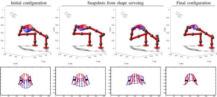
We describe simulated data experiments, for which we used Matlab as well. We developed our code from core functions of the programming language. We considered two KUKA LWR robotic arms manipulating a deformable object. We simulated the object’s deformation using position-based dynamics, which is commonly employed in physics engines. The average execution times per iteration were 120 ms for shape tracking and 37 ms for shape control. We used λ = 0.2. We present results for a paper sheet and a shoe sole.

(7)

Initial configuration Snapshots from shape servoing Final configuration 0 500 1000 1500 2000 2500 3000 0 200 400 600 800 1000 1200 1400 1600

Camera image (pixels)

Current Desired Matches 0 500 1000 1500 2000 2500 3000 0 200 400 600 800 1000 1200 1400 1600

Current Desired Matches

Fig. 5. Shape servoing results. Top: Initial configuration (left), two intermediate configurations during servoing, and final configuration (right). The current (blue) and desired (red) shapes are shown. Bottom: Camera images for the plots on top. The image of the current shape is shown in blue. The matched points appear as filled circles and the patches are shown in black color. The fixed image of the desired shape is also shown overlaid, in red color.

50 100 150 0 50 100 150 Iteration

Shape max. error (mm)

50 100 150 0 5 10 15 20 25 Iteration SfT max. error (mm)

Fig. 6. Shape servoing results. Left: maximum (among all particles) servoing error measured as the difference between the current and the desired shape. Right: maximum (among all particles) error of shape tracking w.r.t. the ground truth for the current shape.

Paper sheet. We modeled a sheet of size A4 with 64

particles. We describe an example of a difficult shape ser-voing task with this object. The task is difficult because the initial and desired shapes are very different, yet the poses of the patches are identical in both shapes. This can be seen in figure 5 (left column). By simply controlling the poses of the patches, the robots would not move at all in this example. In contrast, by taking into account the object’s shape and template, our method can successfully complete the task and servo across this large deformation. To test the robustness of the servoing scheme, we introduced non-idealities such as (i) inaccurate template: we chose β = 0.3 whereas the true value of the parameter for the actual object’s deformation was 1, (ii) incomplete and unstable visual feedback: specifically, a set of between 1 and 10 image point matches changing randomly was used and (iii) additive Gaussian image noise, of standard deviation 3 pixels. The robot motions successfully brought the object to the desired shape despite the perturbations. Figure 6 shows that the proposed scheme completed the servoing within 1 mm shape error even though the final shape perception error was in the order of 10 mm. The presented approach is therefore capable of overcoming inaccuracies in shape perception.

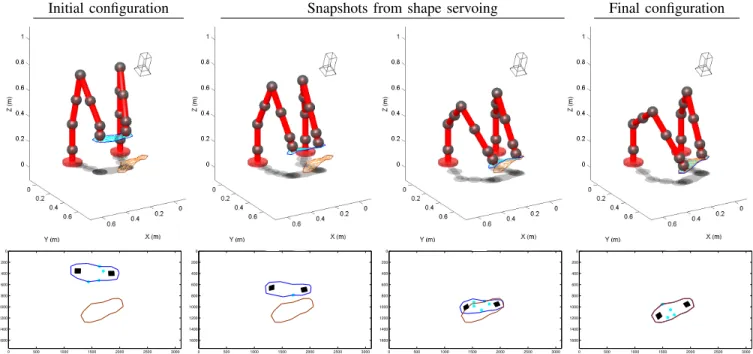
Shoe sole.We modeled a shoe sole with 30 particles. We

changed the gripping setup: this time, the robots grasped the object from above. We included similar perturbations to the previous example: an inaccurate β (0.5 vs. the actual value of 0.8), image noise of 3 pixels, and a set of 1 to 5 random image matches. The results are shown in figures 7 and 8. The robots successfully completed the shape servoing with 10 mm maximum error among all points.

C. Shape servoing experiment

We tested our shape servoing scheme with a robotic arm (Franka Emika Panda) manipulating a rectangular paper sheet. We modeled the sheet with 48 particles. We attached to it two planar rigid pieces thus creating a patch on each of the two shorter sides of the sheet. Note that this is equivalent to using instead rigid planar robotic grippers having the shape of the patch. Each patch contained four particles. One patch was fixed in the environment. The other was grasped by the robot. Only the grasped patch was used for shape control, but both of them were used for shape perception. We used a Dell OptiPlex 5060 computer, with Intel Core i7 CPU and 16 GB RAM. The camera was a Logitech C270 webcam. We used the OpenCV library and Aruco markers for matching. We implemented Algorithms 1 and 2 in Python. We used ROS to control the robot, sending Cartesian end-effector pose commands. In this experiment we captured the desired image with the robot grasping the object. This helped to obtain a precise and reachable desired shape. For the experiment we present, the parameter values were maxIters = 60,

solverIters = 1, ϵ = 10-6_{m, µ = 0.2, ϵ}

c = 0.02 m,

λ = 0.2, β = 0.3. We tested other combinations of parameter values that also provided satisfactory performance.

In figure 9 one can notice the convergence of the shape servoing by the similarity between the superimposed final

(8)

Initial configuration Snapshots from shape servoing Final configuration 0 500 1000 1500 2000 2500 3000 0 200 400 600 800 1000 1200 1400 1600

Current Desired Matches

Fig. 7. Shape servoing results. Top: Initial configuration (left), two intermediate configurations during servoing, and final configuration (right). The current (blue) and desired (brown) shapes are shown. Bottom: Camera images for the plots on top. The image of the current shape is shown in blue. The matched points appear as filled circles and the patches are shown in black color. The fixed image of the desired shape is also shown overlaid, in brown color.

50 100 150 200 250 0 50 100 150 200 250 300 Iteration

Shape max. error (mm)

50 100 150 200 250 0 5 10 15 20 Iteration SfT max. error (mm)

Fig. 8. Shape servoing results. Left: maximum (among all particles) servoing error measured as the difference between the current and the desired shape. Right: maximum (among all particles) error of shape tracking w.r.t. the ground truth for the current shape.

and desired images. The shape tracking was stable and had suitable accuracy to guide the task (see rightmost plot). The shape tracking computation took 56 ms per iteration and the full control loop ran at 69 ms per iteration. There were occlusions as some markers were not visible during servoing. Visibility reached a minimum value of 54% during the task. The results thus illustrate the accuracy, speed and robustness of the proposed servoing scheme. We provide further experimental results in the video attachment.

V. DISCUSSION

A. Why use SfT for shape perception?

One could use, for instance, a depth sensor (e.g., RGBD camera) or Non-Rigid Shape-from-Motion (NRSfM).

Depth sensor. It is usually noisy, works poorly outdoor

and has specific working ranges which might not be adapted for a given task. It cannot sense the occluded parts either.

NRSfM.It does not need a template. However it requires

multiple images to infer the shapes of the object’s common visible surface and only up to scale. It can thus neither infer the occluded parts nor the depth of the desired shape. Therefore it is not adapted to servo the object’s shape.

SfT.For objects that deform isometrically, we recall that

SfT yields the true solution from a single image. SfT can also infer the occluded parts of the object thanks to the template. It allows us to implement the proposed scheme using only a monocular camera. This is important since the monocular camera is the principal sensor in numerous confined space problems where the objects are usually deformable, such as minimally invasive surgery and micro/nano manipulation. B. Convergence of the proposed shape servoing scheme

The proposed robots’ pose control is stable and the shape perception can provably find the true shape. The predicted feasible shape computed at each k by FSI is intended to be an evolution of the current shape towards the desired one. The underlying idea of the strategy Move Robots is that a small current shape evolution requires small patch displace-ments and may thus be reliably reproduced by the patch motions the strategy creates. Thus, the current shape can get

closer to the predicted one, i.e., ||x(k + 1) − xpred(k)|| ≤

||x(k) − xpred_{(k)||. Also, the desired shape is feasible, as it}

is a shape the object itself has taken. Under these facts, the proposed scheme can achieve the desired shape.

C. Servoing through singular shape configurations

λ determines the length of the steps FSI takes towards the desired shape. The smaller λ, the better the object can follow the predicted shapes. However with a small λ a predicted shape might get stuck in a singular configuration or the object might not be able to go across a singular configuration (e.g., flat shape for a paper sheet). On the other hand, the larger λ, the easier it is to go through a singular configuration; but the object might not follow the predicted shapes.

(9)

0 5 10 15 20 0 10 20 30 40 50 60 70 Time (s) RMS of estimated error (mm)

Fig. 9. Shape servoing experiment results. Left to right: the initial image, an intermediate image, and the final image (with the desired image superimposed) during servoing; RMS of the estimated shape servoing error xtr(k)-xdes.

VI. CONCLUSION

The proposed scheme has the advantages of being simple and capable of handling large isometric deformations without requiring complex information. The proposed shape tracking and shape control methods in the scheme are clearly comple-mentary, because they are both based on the template. Still, they can also be used independently. This scheme can be applied to stiff objects such as paper, however one could use it for fabrics as well by taking into account gravity.

As future work we shall address: (i) controlling non-isometric deformations, (ii) upgrading the proposed scheme for volumetric objects, and (iii) studying formally the con-vergence of the proposed scheme.

REFERENCES

[1] D. Navarro-Alarcon and Y.-H. Liu, “Fourier-based shape servoing: A new feedback method to actively deform soft objects into desired 2-D image contours,” IEEE Transactions on Robotics, vol. 34, no. 1, pp. 272–279, 2018.

[2] S. Hutchinson, G. Hager, and P. Corke, “A tutorial on visual servo control,” IEEE Transactions on Robotics and Automation, vol. 12, no. 5, pp. 651–670, 1996.

[3] J. Sanchez, J.-A. Corrales, B.-C. Bouzgarrou, and Y. Mezouar, “Robotic manipulation and sensing of deformable objects in domestic and industrial applications: a survey,” The International Journal of Robotics Research, vol. 37, no. 7, pp. 688–716, 2018.

[4] A. Bartoli, Y. Gérard, F. Chadebecq, T. Collins, and D. Pizarro, “Shape-from-Template,” IEEE Transactions on Pattern Analysis and Machine Intelligence, vol. 37, no. 10, pp. 2099–2118, 2015. [5] F. Brunet, A. Bartoli, and R. Hartley, “Monocular template-based 3D

surface reconstruction: Convex inextensible and nonconvex isometric methods,” Comput. Vis. Image Underst., vol. 125, pp. 138–154, 2014. [6] E. Özgür and A. Bartoli, “Particle-SfT: a Provably-Convergent, Fast Shape-from-Template Algorithm,” International Journal of Computer Vision, vol. 123, no. 2, pp. 184–205, 2017.

[7] D. Navarro-Alarcon, Y.-H. Liu, J. G. Romero, and P. Li, “Model-free visually servoed deformation control of elastic objects by robot manipulators,” IEEE Trans. Rob., vol. 29, no. 6, pp. 1457–1468, 2013. [8] J. Zhu, B. Navarro, P. Fraisse, A. Crosnier, and A. Cherubini, “Dual-arm robotic manipulation of flexible cables,” in IEEE/RSJ Intern. Conf. on Intelligent Robots and Systems, 2018, pp. 479–484.

[9] D. Navarro-Alarcon, Y.-H. Liu, J. G. Romero, and P. Li, “On the visual deformation servoing of compliant objects: Uncalibrated control meth-ods and experiments,” International Journal of Robotics Research, vol. 33, no. 11, pp. 1462–1480, 2014.

[10] C. Shin, P. W. Ferguson, S. A. Pedram, J. Ma, E. P. Dutson, and J. Rosen, “Autonomous tissue manipulation via surgical robot using learning based model predictive control,” in IEEE International Conference on Robotics and Automation, 2019, pp. 3875–3881. [11] F. Alambeigi, Z. Wang, R. Hegeman, Y.-H. Liu, and M. Armand,

“Autonomous data-driven manipulation of unknown anisotropic de-formable tissues using unmodelled continuum manipulators,” IEEE Robotics and Automation Letters, vol. 4, no. 2, pp. 254–261, 2019.

[12] B. Jia, Z. Hu, J. Pan, and D. Manocha, “Manipulating highly de-formable materials using a visual feedback dictionary,” in IEEE Int. Conf. on Robotics and Automation, 2018, pp. 239–246.

[13] A. R. Fugl, A. Jordt, H. G. Petersen, M. Willatzen, and R. Koch, “Simultaneous estimation of material properties and pose for de-formable objects from depth and color images,” in Pattern Recognition. DAGM/OAGM 2012. LNCS, vol. 7476, Springer, A. Pinz, T. Pock, H. Bischof, and F. Leberl, Eds., 2012, pp. 165–174.

[14] J. Schulman, A. Lee, J. Ho, and P. Abbeel, “Tracking deformable objects with point clouds,” in IEEE International Conference on Robotics and Automation, 2013, pp. 1130–1137.

[15] A. Petit, V. Lippiello, G. A. Fontanelli, and B. Siciliano, “Tracking elastic deformable objects with an RGB-D sensor for a pizza chef robot,” Robotics and Auton. Systems, vol. 88, pp. 187–201, 2017. [16] T. Han, X. Zhao, P. Sun, and J. Pan, “Robust shape estimation for 3D

deformable object manipulation,” Communications in Information and Systems, vol. 18, no. 2, pp. 107–124, 2018.

[17] C. Elbrechter, R. Haschke, and H. Ritter, “Bi-manual robotic paper manipulation based on real-time marker tracking and physical mod-elling,” in IEEE/RSJ International Conference on Intelligent Robots and Systems, 2011, pp. 1427–1432.

[18] T. Collins and A. Bartoli, “Realtime Shape-from-Template: System and Applications,” in IEEE International Symposium on Mixed and Augmented Reality, 2015, pp. 116–119.

[19] D. Navarro-Alarcon, H. M. Yip, Z. Wang, Y.-H. Liu, F. Zhong, T. Zhang, and P. Li, “Automatic 3D manipulation of soft objects by robotic arms with adaptive deformation model,” IEEE Transactions on Robotics, vol. 32, no. 2, pp. 429–441, 2016.

[20] S. Kagami, K. Omi, and K. Hashimoto, “Alignment of a flexible sheet object with position-based and image-based visual servoing,” Advanced Robotics, vol. 30, no. 15, pp. 965–978, 2016.

[21] Z. Hu, P. Sun, and J. Pan, “Three-dimensional deformable object manipulation using fast online Gaussian process regression,” IEEE Robotics and Automation Letters, vol. 3, no. 2, pp. 979–986, 2018. [22] Z. Hu, T. Han, P. Sun, J. Pan, and D. Manocha, “3-D deformable

object manipulation using deep neural networks,” IEEE Robotics and Automation Letters, vol. 4, no. 4, pp. 4255–4261, 2019.

[23] S. Duenser, J. M. Bern, R. Poranne, and S. Coros, “Interactive robotic manipulation of elastic objects,” in IEEE/RSJ International Conference on Intelligent Robots and Systems, 2018, pp. 3476–3481.

[24] F. Ficuciello, A. Migliozzi, E. Coevoet, A. Petit, and C. Duriez, “FEM-based deformation control for dexterous manipulation of 3D soft objects,” in IEEE/RSJ International Conference on Intelligent Robots and Systems, 2018, pp. 4007–4013.

[25] J. Das and N. Sarkar, “Autonomous shape control of a deformable object by multiple manipulators,” Journal of Intelligent & Robotic Systems, vol. 62, pp. 3–27, 2011.

[26] P. Jiménez, “Survey on model-based manipulation planning of de-formable objects,” Robotics and Computer-Integrated Manufacturing, vol. 28, no. 2, pp. 154–163, 2012.

[27] M. Müller, B. Heidelberger, M. Hennix, and J. Ratcliff, “Position based dynamics,” Journal of Visual Communication and Image Representa-tion, vol. 18, no. 2, pp. 109–118, 2007.

[28] J. Bender, M. Müller, M. A. Otaduy, M. Teschner, and M. Macklin, “A survey on position-based simulation methods in computer graphics,” Computer Graphics Forum, vol. 33, no. 6, pp. 228–251, 2014. [29] F. Chaumette and S. Hutchinson, “Visual servo control. I. Basic

approaches,” IEEE Robotics & Automation Magazine, vol. 13, no. 4, pp. 82–90, 2006.