Scheduling in production, supply chain and Industry 4.0 systems by optimal control: fundamentals, state-of-the-art and applications

HAL Id: hal-01998181

https://hal.archives-ouvertes.fr/hal-01998181

Submitted on 29 Jan 2019

HAL is a multi-disciplinary open access archive for the deposit and dissemination of sci-entific research documents, whether they are pub-lished or not. The documents may come from teaching and research institutions in France or abroad, or from public or private research centers.

L’archive ouverte pluridisciplinaire HAL, est destinée au dépôt et à la diffusion de documents scientifiques de niveau recherche, publiés ou non, émanant des établissements d’enseignement et de recherche français ou étrangers, des laboratoires publics ou privés.

Scheduling in production, supply chain and Industry 4.0

systems by optimal control: fundamentals,

state-of-the-art and applications

Alexandre Dolgui, Dmitry Ivanov, Suresh Sethi, Boris Sokolov

To cite this version:

Alexandre Dolgui, Dmitry Ivanov, Suresh Sethi, Boris Sokolov. Scheduling in production, supply chain and Industry 4.0 systems by optimal control: fundamentals, state-of-the-art and applica-tions. International Journal of Production Research, Taylor & Francis, 2019, 57 (2), pp.411-432. �10.1080/00207543.2018.1442948�. �hal-01998181�

Scheduling in production, supply chain and Industry 4.0 systems by optimal control: fundamen-tals, state-of-the-art, and applications

Alexandre Dolgui1 , Dmitry Ivanov2*, Suresh Sethi3, Boris Sokolov4,5 1

Automation, Production and Computer Sciences Dept. IMT Atlantique LS2N - CNRS UMR 6004 La Chantrerie

email: alexandre.dolgui@imt-atlantique.fr 2*

Berlin School of Economics and Law

Department of Business Administration; Professor for Supply Chain Management 10825 Berlin, Germany

Phone: +49 30 85789155 E-Mail: divanov@hwr-berlin.de

3

Eugene McDermott Chair

Center for Intelligent Supply Networks (C4iSN) Naveen Jindal School of Management, Mail Station SM30

The University of Texas at Dallas

800 W. Campbell Rd., Richardson, Texas 75080-3021 E-mail: sethi@utdallas.edu

4

Saint Petersburg Institute for Informatics and Automation of the RAS (SPIIRAS) V.O. 14 line, 39 199178 St. Petersburg, Russia

E-Mail: sokol@iias.spb.su 5

ITMO University, St. Petersburg, Russia E-Mail: sokol@iias.spb.su

* Corresponding author Dmitry Ivanov

Abstract

Specific scheduling problems with complex hybrid logical and terminal constraints, non-stationarity in process execution as well as complex interrelations between dynamics in process design, capacity utili-zation, and machine setups require further investigation and the application of a broad range of method-ical approaches. One of these approaches is optimal control. The objectives of this survey are twofold. The first objective is to derive major contributions, application areas, limitations, as well as research and application recommendations for the future regarding optimal control applications to scheduling. The second objective is to explain control engineering models in terms of industrial engineering and produc-tion management. In this paper, we provided a survey on the applicaproduc-tions of optimal control to schedul-ing in production, supply chain, and Industry 4.0 systems with a focus on the deterministic maximum principle. Optimal control approaches take a different perspective as mathematical programming meth-ods which represent schedules as trajectories. We consider optimal control models, performance analy-sis qualitative methods, and computational methods for optimal control. We provide a brief historic overview and clarify major mathematical fundamentals whereby the control engineering terms are brought into correspondence with industrial engineering and management. The survey allows the group-ing of models with only terminal constraints with application to master production schedulgroup-ing, models with hybrid terminal-logical constraints with applications to short term job and flow shop scheduling, and hybrid structural-terminal-logical constraints with applications to customized assembly systems such as Industry 4.0. Computational algorithms in state, control, and adjoint variable spaces are dis-cussed. Finally, we derive major contributions, application areas of different control methods, and their limitations. This paper also provides recommendations for future research and applications.

Keywords: optimal program control, deterministic control, maximum principle, scheduling, attainable sets, algorithms

1. Introduction

Short-term scheduling belongs to the fundamentals of scheduling theory. It considers jobs containing operation chains with equal (i.e., flow shop) or different (i.e., job shop) machine sequences and different processing times. The operations need to be scheduled for machines with different processing power subject to some criteria such as makespan, lead time, or due dates (Blazewicz et al. 2001, Pinedo 2008, Dolgui and Proth 2010, Werner and Sotskov 2014).

Over the last decades, mathematical optimization applications to scheduling problems have been studied from different perspectives whereby significant progress can be observed in the development of rigor-ous theoretical models and efficient solution techniques. Lauff and Werner (2004), Jungwattanakit et al. (2009), Sotskov et al. (2013), Choi et al. (2013), Harjunkoski et al. (2014), Bożek and Wysocki (2015), Ivanov et al. (2016a,c) have pointed out that specific scheduling problems with complex hybrid logical and terminal constraints, non-stationarity in process execution as well as complex interrelations between dynamics in process design, capacity utilization, and machine setups require further investigation and the application of a broad range of methodical approaches.

Optimal control approaches take a different perspective as mathematical programming methods which represent schedules as trajectories. Optimal control applications to scheduling problems are encountered in production systems with single machines (Giglio 2015), job sequencing in two-stage production sys-tems (Lou and Van Ryzin 1989, Sethi and Zhou 1996) and multi-stage machine structures with alterna-tives in job assignments and intensity-dependent processing rates such as flexible manufacturing sys-tems (Sharifnia et al. 1991, Maimon et al. 1998, Yang et al. 1999, Ivanov and Sokolov 2013a, Pinha et al. 2015), supply chains as multi-stage networks (Ivanov and Sokolov 2012, Ivanov et al. 2013), and Industry 4.0 systems based on data interchange between the product and stations, flexible stations dedi-cated to various technological operations, and real-time capacity utilization control (Ivanov et al. 2016a).

This survey considers research on optimal control applications to production scheduling with analysis of model parameters and computational algorithms published in the last 55 years. The objectives of this survey are twofold. The first objective is to derive major contributions, application areas, limitations, as well as research and application recommendations for the future regarding optimal control applications to scheduling. The second objective is to explain control engineering models in terms of industrial engi-neering and production management. We provide a survey on the applications of optimal control to scheduling in production, supply chain, and Industry 4.0 systems whereby we restrict ourselves to de-terministic maximum principle-based approaches and omit detailed analysis of stochastic optimal con-trol approaches as well as dynamic programming algorithms. Regarding the related topics which are not covered in this paper, we refer to the surveys by Sethi (1978, 1984) for applications of the maximum principle to production-inventory problems and to works (Lou et al. 1994, Sethi and Zhang 1994, Presman et al. 1995, Samaratunga et al. 1997, Presman et al. 1997, 2000, Feng and Yan 2000, Sethi et al. 2002, Khmelnitsky et al. 2011) which extend this survey to stochastic scheduling problems.

The survey follows the structure “optimal control models – performance analysis qualitative methods – computational methods”. In Section 2, a brief historic overview and clarification of major mathematical fundamentals are provided. The control engineering terms are brought into correspondence with indus-trial engineering and management. In Section 3, optimal control models for scheduling in production, supply chain, and Industry 4.0 systems are presented and classified in terms of their analytical contents

and application areas. Section 4 deals with attainable (reachable) sets as a method of qualitative analysis of optimal control performance. Section 5 is devoted to computational algorithms regarding state, con-trol, and adjoint variable spaces. In Section 6, we derive major contributions, application areas of differ-ent methods, and their limitations. This section also provides recommendations for future research and applications. The paper concludes in Section 7 by summarizing the insights from this survey.

2. Fundamentals of optimal control models with applications to scheduling

2.1. Historical development

Optimal control approaches represent schedules as trajectories. The first studies in this area were devot-ed to inventory control. One of these studies (Eilon 1961) was publishdevot-ed in the first volume of the

Inter-national Journal of Production Research (IJPR). Later, Hwang et al. (1967, 1969) were among the first

to apply optimal control and the maximum principle to multi-level and multi-period master production scheduling which determined the optimal control (i.e., production) with the corresponding state (i.e., inventory) trajectory. Albright and Collins (1977) developed a Bayesian approach to the optimal control of continuous industrial processes. Bedini and Toni (1980) developed a dynamic model for the planning of a manufacturing system. The maximum principle has been used to formulate the problem and obtain a solution. A large research area of flexible manufacturing systems and their dynamics has been exam-ined in numerous studies (e.g., Stecke and Solberg 1981). The stream of production scheduling was continued by Kimemia and Gershwin (1985), Kogan and Khmelnitsky (1996), and Khmelnitsky et al. (1997), who applied the maximum principle in discrete form to the planning of continuous-time flows in flexible manufacturing systems

The origins of control scheduling techniques can be found in network planning, dynamic programming and waiting line theory (Moiseev 1974, Sotskov et al. 2013). Consider the graph in Fig. 1.

х1 х2 х3 х5 х4 х6 хп–2 хп–1 хп

Fig. 1. Network planning graph

In the classical network planning theory, the state x_i of the i-job can be determined subject to Eq. (1):

i i i i Q T x    , (1)

where Ti is the task time to process the i-job, Qi is the processing volume of the i-job, and i is the

in-tensity (i.e., processing rate) of processing the i-job, whereby the jobs i= 1,...,n are interconnected with each other in terms of precedence constraints “or”/“and”. It is notable that even if elements of dynamics can be observed in the aforementioned system regarding process deployment in time, job execution dynamics itself have not been considered explicitly. In other words, operations execution has been treat-ed in a static manner since task times nwere assumtreat-ed to be fixtreat-ed. In reality, task times may change in job execution dynamics. As such, dynamics of job execution requires an explicit description of job pro-cess execution, distribution (allocation) of resources required for job execution, and changes in the job states and the respective control inputs. The aforementioned dynamic interpretation of job execution was extensively developed in the 1970s (Zimin and Ivanilov 1971, Moiseev 1974) within the framework of optimal control theory.

Optimal control theory is devoted to determining some functions known as controls that lead to optimi-zation(minimization or maximization) of an objective (Pontryagin et al. 1964, Athaus and Falb 1966, Lee and Markus 1967, Moiseev 1974, Bryson and Ho 1975, Hartl and Sethi 1984, Soner 1986, Gersh-win 1994, Sethi and Thompson 2000). This theory evolved over the centuries based on calculus varia-tion principles developed by Fermat, Lagrange, Bernulli, Newton, Hamilton and Jacobi. In the 20th cen-tury, two computational fundamentals of optimal control theory, the maximum principle (Pontryagin et al., 1964) and the dynamic programming method (Bellmann 1972), were developed. These methods extend the classical calculus variation theory which is based on control variations of a continuous trajec-tory and observing the performance impact of these variations at the trajectrajec-tory end. Since control sys-tems in the middle of the 20th century were increasingly characterized by piecewise continuous func-tions (such as 0-1 switch automats), the development of the maximum principle and the dynamic pro-gramming was needed for solving problems with complex constraints on state and control variables. This section aims to clarify the notions of state, control, and performance at the optimal control model level, bridging these notions to industrial management and engineering. Moreover, the computational level will be considered and the maximum principle, adjoint equation system, and transversality condi-tions will be clarified.

2.2. Major elements of an optimal control model for scheduling

Consider the evolution of a quantifiable object (e.g., inventory or production quantity) in time ), u ), ( x , ( f ) ( xt  t t t t t_f dt d t) x, ₀   ( x

where uRmis the control,

x



R

nis the terminal system state vector, fRnis a given function,

R

nis Euclid space of dimensionality

n

,t

₀is the initial point in time and t_f is final point in time. For exam-ple, in a job shop, x t( )can describe a buffer such as production quantity or inventory, and control variableu(t)can describe processed flow volume of a job at a machine. The system state vector is de-termined by the evolution of state variables x t( ) that characterize the system at each point in time. State evolution in dynamics is determined by control variables u(t) that correspond to the decisions of a per-son or an algorithm governing the system dynamics.

In real practice of control engineering, control variables are typically considered bounded piecewise continuous functions. Examples of controls in operational systems include processing rates ofmachines in manufacturing or shipment rates in transportation. In production scheduling, binary control variables are used to describe the assignment of a job to a machine. Consider an example (Fig. 2).

(t)=1 1 2 3 4 5 6 7 6 5 4 3 2 0 t 8 9 1 ) (t x 10 11 12 13 (t)=1 (t)=1 1 ) ( ; ) ( 2 1 t c u t  u ) (t x

Figure 2. Example of job execution dynamics

Fig. 2 represents job execution dynamics in which the non-stationarity of job execution is reflected. Machine availability times (subject to maintenance or other restrictions) are given as a preset matrix time function (t). The

u

₁

(

t

)

is a control decision variable characterizing the processed flow volume at the machine subject to some processing intensity and to another control decision

u

₂

(

t

)



1

, namely an assignment of the job to this machine. It can be observed in Fig. 2 that job processing at the machine starts at

t 

t

₁ and ends at t t₁₁ whereby a flow (volume) of six product units is produced.

A standard dynamic network process control model has the form of Eqs. (2)-(8).

Mathematical model of job execution control





























_

_

        1 2

)

(

)

(

)

(

( ) ( ) ( ) ( ) ( ) ( ) ) ( ) ( ) ( i i o o o o o i o i o i o i o i

_x

_u

_a

_x

_x

_a

_x

_a

dt

dx

     









(2) where ( o) i

x is the current state of the execution of the i-job, _(a_i(o)x_i(o)) are asymmetric step func-tions that set logical constraints to avoid overproduction in regard to the planned volume ( o)

i a (see fur-ther in Eq. 4),





          1 2 i i o o o o _{a x a} x       

 ( ( ) ( )) ( ( ) ( )) are asymmetric step functions that set logical precedence constraints “and”/“or” regarding the i-job (cf. Eq. 5). The job numbers  and  from the sets 

_i1 _i₂determine preceding jobs for the i-job. u_i( o)is a continuous control variable subject to the maximum processing intensity of operations execution (Eq. 3).

) ( ) ( o i o i c u   0 (3)

The peculiarity of optimal control models are constraints. In practice, the system trajectory cannot be-long to some areas in the space

R

n. The above-mentioned boundary conditions belong to the con-straints on the trajectory that can differ regarding fixed or free ends. In scheduling models, we typically have fixed end boundary conditions (Eq. 7). Next, the constraints on control need to be defined. Since the search for optimal control is performed within the class of functions u(t) that depend only on t, this problem class is called optimal program control. Typically, in production scheduling we have optimal program control problems with two types of constraints on control, i.e., terminal and logical constraints. In future systems of Industry 4.0 production, the third type of hybrid constraints, i.e., structural-logical-temporal constraints will be used (see further in this paper in Sect. 3.3). Terminal constraints (see Sect. 3.1 in this paper) describe limited control resources (e.g., Eqs. 4 and 5). An example of a terminal con-straint is a capacity restriction at a machine. Logical concon-straints (see further in this paper in Sect. 3.2) describe α-precedence relations of the type “or” and β-precedence relations of the type “and” regarding the job sequences in the jobs (Eq. 5).

) (a_i(o)x_i(o) 



{0,1} (4)





          1 2 i i o o o o _{a x a} x         ( ( ) ( )) ( ( ) ( )) {0,1} (5)

Terminal constraints (4) describe restrictions for limiting job execution subject to fixed processing vol-umea_i(o). Constraints (5) determine precedence relations by blocking job

D

until the previous opera-tions D ,_ D_ have been completed. Optimal control scheduling models with only terminal constraints typically address the master production scheduling level (Hwang et al. 1967, 1969, Kimemia and

Gershwin 1983, Jiang and Sethi 1991, Khmelnitsky et al. 1997, Kogan and Khmelnitsky 2000). Sched-uling models with both terminal and logical constraints can also be applied to flow shop and job shop scheduling (Kalinin and Sokolov 1985, 1987, Ivanov and Sokolov 2013a, Ivanov et al. 2016a,с) as well as to supply chain scheduling (Ivanov and Sokolov 2012, Ivanov et al. 2013). Along with constraints (3), integral constraints on resources are typically written in the form of Eq. (6):



 f t t dt u t x t F 0 0 ) ), ( , ( (6)

In order to assess the scheduling results, optimal control models define boundary conditions, i.e., start and end conditions such as Eq. (7)

0

x

h

0

x

h

₀

(

(

t

₀

))



;

₁

(

(

t

_f

))



, (7) where

h

(₀o), h₁(o) are known differentiable functions that determine the start and end conditions of the vector x(t). For example, an initial condition might specify that the executed volume of jobs at the beginning of the scheduling horizon is equal to zero. End conditions could reflect the desired end state, i.e., the completion of the jobs by the time tf.

The optimal program control vector

u

(t

)

and the state trajectory xf(x,u,t)should be determined so that the boundary conditions are met; in other words, the desired values of the scheduling performance indicators should be achieved as an analogy to goal programming.

The performance assessment is designed in control systems in the following way. The control of system (2) is directed towards attainability of some performance. The performance metrics (or functionals, in terms of optimal control) can be grouped into terminal (i.e., flow-oriented metrics, e.g., work-in-process inventory or planned production volume subject to a customer demand) and integral (e.g., due dates) functionals (Eq. 8):





    f t t n i f o i o i x t d a J 0 )) ( ( )) ( ( 1 2 ) ( ) (







u (8)

Performance reachability depends on the selection of the trajectory x(t) and control

u

(t

)

. In general, scheduling problems in terms of control have been formulated for searchingoptimal program control for dynamic system (2) subject to minimization of the functional (8) subject to constraints (3)-(7). The first term in Eq. (8) characterizes the relationship between planned job execution volume and the volume that can be realized in the computed schedule. The second term depends on the interpretation of the function

) (

(





u and frequently plays the role of delay penalties.

2.3. Major elements of optimal control computational procedures

Necessary optimality conditions can be derived from the maximum principle (Sethi 1978, Hartl et al. 1995, Afanasiev et al. 1996, Khmelnitsky et al. 1997, Sethi and Thompson 2000). Consider control sys-tem (9): )), ( u ), ( x , ( ) ( xt  f t t t t₀ tt_f, x(t₀)x₀,

u

(

t 

)

U

,

J F(x(tf))min (9)

Let us introduce a scalar Hamiltonian function

H

and adjoint vector system Rnin Eq. (10): )), ( u ), ( x , ( f ) ( )) ( ), ( u ), ( x , (t t t t t t t t H  

)), ( ), ( u ), ( x , ( x ) (t H t t t t       (10) , x )) ( x ( ) ( f t t f t F t       (11)

Adjoint vector system plays the role of dual models in linear programming. Coefficients of the adjoint systems can be interpreted as Lagrange multipliers. Under assumptions that u t( ) is optimal control and

) (

x t and (t)are the trajectory and adjoint system satisfying (10) and (11), the function

)) ( ψ ), ( u ), ( x , (t t t t

H reaches its maximum for x t( )at the pointu t( ). Then Eq. (12) holds:

)) ( ψ ), ( x , ( u u t t t (12)

Subsequently, Eq. (12) is brought into correspondence with (10) and (11). As a result, a two-point boundary problem for a system of ordinary differential equations involving x t( ) and (t) is formed. The optimal solution is now bounded by this differential system. Note that Eqs. (9)-(12) in general pro-vide only the necessary conditions for the existence of an optimal solution. For linear control systems, these maximum principles provide both optimality and the necessary conditions (Ivanov and Sokolov 2010). This fact requires further optimality study for each concrete case of application.

Typically, computational procedures start with a nominal solution that satisfies both main and adjointdifferential systems. Then this solution is modified by integrating main and adjoint systems by control variations towards a Hamiltonian increase. During this procedure, at

t 

T

_f transversality condi-tions are evaluated. Transversality condicondi-tions are the end condicondi-tions of the adjoint system. The adjoint variables can be interpreted as dynamic priorities of jobs and play here the role of “shadow” prices in linear programming models. However, in contrast to those canonical forms where “shadow” prices are fixed, the adjoint variables change dynamically. These changes are subject to the contribution of a par-ticular operations assignment and scheduling (i.e., machine and time windows) to the change in perfor-mance assessment functions. Consequently, at each point in time the dynamic priorities of jobs may be changed if a newly arrived job provides a better contribution to the performance functional.

Various algorithms based on Pontryagin’s maximum principle have been developed in the aforemen-tioned area. In essence, these algorithms reduce the non-classical calculus variation problem to a two-point boundary problem (Zimin and Ivanilov 1971, Moiseev 1974). Regarding large-scale problems, two major shortcomings of this approach have been observed. First, the two-point problem became a multiple-point problem with jumps in the adjoint variables at the end of job processing because of ter-minal constraints (4). The explanation of this effect can be seen in step function differentiating. The step functions became general delta-functions. The second problem was related to the numerical computa-tion of the boundary problems for deriving the initial condicomputa-tions of the adjoint variables which are need-ed to compute the optimal schneed-edule. Questions of convergence, optimality, and the necessary conditions remained open. Special heuristic algorithms were developed in this area to overcome these problems (Chernousko & Lyubushin (1982).

In order to resolve the problems with the step functions and the respective non-linearity in the right-hand parts of Eq. (2), Moiseev (1974) and Kalinin and Sokolov (1985)] developed another variant to describe the right-hand parts of Eq. (2) as terminal constraints in the control and functional space (Eq 13), whereby the functional (8) was modified as shown in Eq. (14).

0 ) ( ) ( 1 2 ) ( ) ( ) ( ) ( ) (             

_

_

   _i _i o o o o o i i x a x a x d       (13)

 

   f t t n i i i p J fd d J 0 1 ) (





, (14)

where

f

_iare given penalty functions if the conditions (13) are not fulfilled (in case of objective function minimization).

d

_iare the given terminal constraints.

The additional component in (14) describes the penalty for non-fulfillment of the condition (13). How-ever, the search complexity for



_i was similar to the search complexity for the jump values in the adjoint variables. In addition, the classical optimal control models for scheduling do not consider as-pects such as setups, indivisibility of resources for job execution at any point of time, and bans on inter-ruptions of the job execution. A special group of problems can be considered regarding uncertainty and risks, schedule stability, flexibility and robustness analysis, as well as multi-criteria resolution. The fol-lowing Section 3 will describe how the given problems can be resolved through several modifications of the model (2)-(8).

3. Optimal control models for job scheduling in production, supply chain, and Industry 4.0 Scheduling problem statements differ in terms of fixed or variable process and operations sequences. In this regards, we structure the analysis in this section in accordance to Fig. 2.

Fig. 2. Classification of scheduling problems solved by optimal program control

Let us analyse the problem statements, models, and algorithms in Sects 3.1-3.3 in detail.

3.1. Model with terminal constraints

According to Kimemia and Gershwin (1983), Kogan and Khmelnitsky (1996), Khmelnitsky et al. (1997) and Maimon et al. (1998), the optimal control model with terminal constraints can be applied to production scheduling in the following settings.

Problem description

The task consists of scheduling jobs on machines subject to cost minimization and on-time demand fulfillment regarding quantity and due date with limited machine capacity considerations.

The problem formalization is presented as follows. Note that, in line with the referenced studies Kogan and Khmelnitsky (1996), Khmelnitsky et al. (1997) and Maimon et al. (1998), Sect. 3.1 contains origi-nal notations which are different from notations in other sections of this paper and are valid for Sect. 3.1 only.

Set indexes

f

t

time of the planning horizon

i

product index,

i1....,l

k

machine index,

_{k }

₁

_,...,

_J

₍

_k

_);

j

machine state index,

j 

1

,....

J

(

k

);

m

job index, m 1,....M(i); Parameters

im

D due date of job

im

X demand

kj

T minimum setup time

ikj



capacity of machine k being in state j when producing product i (in case of product consumption, this parameter is negative)

c i

c

subcontracting cost per unit product

c

_ir ;

r i

c

purchasing cost of all raw materials required per unit product

_i

; p

im

c

penalty for violating the due date of job

_m

Decision variables

) (t

X_i cumulative buffer level of i-product at time

t

_;

)

(t

V

_kj a dimensionless continuous function that reflects the current state of machine; V_kj(t)[0;1]

)

(t

w

kj control variable characterizing actual loading of machine

k

relative to its production capacity

];

1

,

0

[

)

( 

t

w

kj ) (t

ukj control variable, characterizing the rate of state j on machine

k

, i.e., the setup rate

Process control model

ikj kj kj i t w t X ()

_

( )



 , (15) ) ( ) (t u t Vkj  kj  , (16)

Eq. (15) describes production process. Eq. (16) describes the setup process.

Constraints

The setup process is characterized by two types of constraints. First, the rate of transformation from current state is equal to the transformation rate into a new state (Eq. 17)

k j kj t u  



( ) 0, . (17)

Second, the rate of transformation from and to state

j

is bounded (Eq. 18) 1 1     T_kj u_kj(t) T_kj , (18)

where

T

kj is the minimum time of setting up machine k on state j , and T is the minimum time of kj

setting down machine k on state j . Eq. (17) characterizes the balance between the setup intensities of

the j-machine by state transition. Eq. (18) constraints the maximum intensity (i.e., processing speed) of the operation processing at the j-machine.

A restriction on sequence-dependent setup process interaction (19) states that the j-machine in the setup state cannot execute processing operations at the same time.

) ( )) ( (wkj t Vkj t   0 , (19) where

_

_(w

₎

is the step (Heaviside) function, i.e.,

 w( )1if

w



0

;



(

w

)



0

,

if

w



0

. Objective function





_















             im im i im p im t i i i r i i c i kj i i kj kju t CX t dt c X c X T X c X X D c f 2 0 2 5 ₀ 2 1 0 0 2 1 ) ) ( , (max )) ( ) ( ( ) ( ( )) ( ( )) ( ( min , (20)

where

X

_i

(t

)

ispositive, and the function

_C

_{( X}

₎

reflects the inventory carrying cost. Otherwise, it re-flects the stock out cost for subproducts (internal shortages) and penalties for violating demands for end products (external shortages)



( ) ( )



)) ( (X t b X t h t C _i  _i1 _i  _i 2 1 , if Xi(t)hi(t)0,



( ) ( )



)) ( (X t b X t h t C _i  _i2 _i  _i 2 1 , if Xi(t)hi(t)0, and _{h is written i}



,

(

)

(

)



min

max

)

(

_{m im i im im} i

t

X

X

D

t

D

h







.

The scheduling problem is now formulated in the following way: minimize the functional constraints (20) to transit the dynamic object (14)-(15) from the given initial state (0), (0)

i

k

i V

X to the required final state (defined in Eq. (20)) subject to constraints (17)-(18).

With the help of the maximum principle, Kogan and Khmelnitsky (1996), (2000) formulated the Hamil-tonian function (21) and the respective adjoint equation systems (22).

















  kj i kj i kj ikj kj x i kj v kj i kj s kj u t C X t t u t t w t v c H ( ( ))2 ( ( ))  ( ) ( )  ( ) ( ) 2 1 , (21)



, ( )



) ( ) (max )) ( ( ) ( _im m im i im p im i x v kj t C X t dt c X X D d t D d   



0    , _i(T )0 0, (22)

)

(

)

(

)

(

t

a

t

dt

d

t

d



V_kj





_kj





_kj ,



_kjV

(

T



0

)



0

.

As a result of Hamiltonian maximization, it becomes possible to compute the optimal schedule for mate-rial flow processing at a machine complex. The schedule is described using three logical conditions regarding control w (Eq. 23):

)

(t

v

_kj , if





i vikj x i

(

t

)

v

0



0

))

(

(

w

t



f

_{n kj} , if





i vikj x i

(

t

)

v

0





0,Vkj(t)



, if





i vikj x i

(

t

)

v

0



(23)

Eq. (23) was derived in the studies by Kogan and Khmelnitsky (1996) and (2000). It underlines the ad-vantages of the maximum principle as compared to other optimal control approaches. The developed approach allows explicit determination of information about the structure of optimal operating modes of work stations prior to computational experiments. In addition, existence conditions were found, i.e., conditions where the Hamiltonian function equals Eq. (21). Kogan and Khmelnitsky (1996) provided evidence of the practical application of the developed approach for a flexible manufacturing system with four machines and six jobs for the case of fixed job processing technology.

A number of questions have arisen from the analysis of the aforementioned approach. First, the compu-tation error estimation as a consequence of replacing the step function in Eq. (19) with a sequence of approximated functions needs to be named. Second, the convergence in the numerical computation pro-cedure needs to be analysed. The Hulquist’s (1988) modification does not guarantee convergence for the considered form of non-linear systems in general. The selection of the initial conditions for the adjoint system is an important precondition for algorithmic convergence. In addition, optimality proofs need to be addressed. As known, the maximum principle for non-linear dynamic systems is a necessary optimal-ity condition. The sufficiency condition needs to be analysed separately (Athaus and Falb 1966, Bryson and Ho 1975, Pontryagin et al. 1964).

At the same time, it can be observed that the initial model (2)-(8) has been extensively extended by the model (15)-(23). Another extension in Sect. 3.2 will be made regarding the dynamic system (15)-(16) itself and the technical and technological constraints (Eq. 17 and 18) subject to practical needs of real-time job and flow shop environments.

3.2 Model with hybrid terminal-logical constraints: applications to job shop and flow shop scheduling

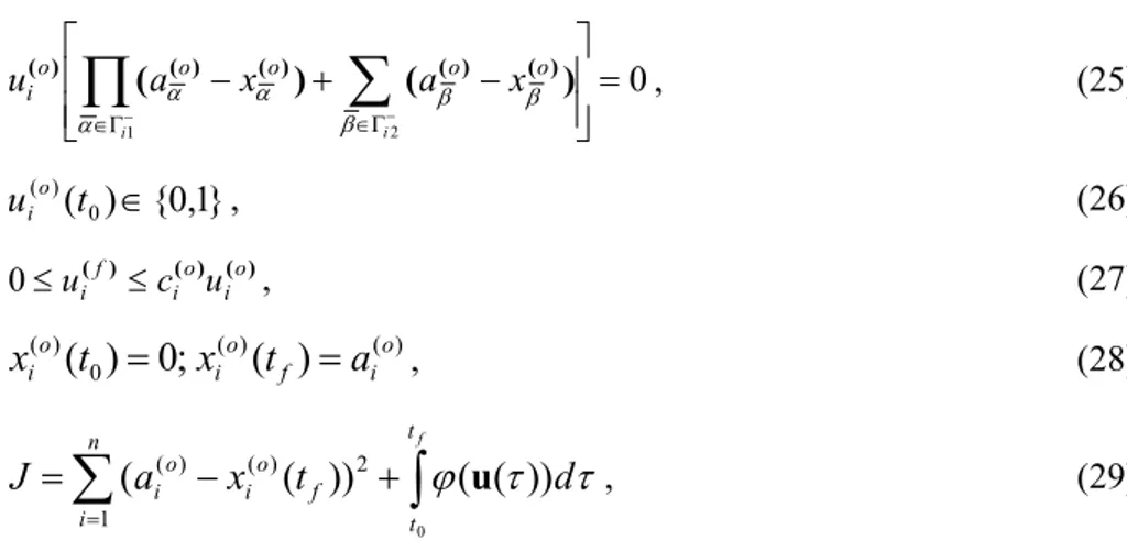
The model in Sect. 3.1 has been proved to be a working tool for production scheduling when flow con-trol is considered and no precedence operation relations exist in jobs. For job shop scheduling, prece-dence relations exist. The studies by Kalinin and Sokolov (1985), (1987), Sokolov and Yusupov (2002) resolved the aforementioned problems with multiple criteria, bans on execution interruptions and non-stationarity for large-scale scheduling problem. The following studies by Ivanov and Sokolov (2013), Ivanov et al. (2013), and Ivanov et al. (2016a,b,c) developed a special form of hybrid terminal-logical constraints that allows the application of maximum principle-based optimal control models to job and flow shop scheduling for flexible manufacturing systems, supply chains, and Industry 4.0 networks. Consider the following simplified example that unites the model of operation execution control and flow control (Eqs. 24-29). ) ( ) ( ) ( ) ( ; _in _if o i o i u x u x    ; (24)

0 1 2            





   i i o o o o o i a x a x u       ) ( ) ( ( ) ( ) ( ) ( ) ) ( , (25) } 1 , 0 { ) (₀ ) (  t uio , (26) ) ( ) ( ) ( o i o i f i c u u   0 , (27) ) ( ) ( 0 ) (

)

(

;

0

)

(

_io _{f i}o o i

t

x

t

a

x





, (28)





    f t t n i f o i o i x t d a J 0 )) ( ( )) ( ( 1 2 ) ( ) (







u , (29)

In contrast to constraints (5) and (13), Eq. (25) contains both control and state variables from Eq. (24). In this form, constraints (25) are new in optimal control applications to scheduling and allow the use of optimal control for assignment and sequencing tasks. In the following part of this paper, we will show how to transit from impulse controls in Eq. (26) to interval [0,1] for these controls in the class of piece-wise continuous functions. The controls will take binary values that will allow their usage in assignment problems. In terms of sequencing, we observe that in Eq. (27), the controls from Eq. (24) are contained. These controls activate Eq. (27) that describes the flow distribution control problem and sequencing subject to processing intensity of the machines. The given constraint system unifies two large model classes: the flow models in system dynamics and operation control and resource distribution models in network planning theory.

The basic idea of this approach is that operation execution and machine availability are dynamically distributed in time over the planning horizon. As such, not all operations and machines are involved in decision making at the same time (Fig. 3).

Fig. 3. Schedule execution dynamics at two points in time (based on Ivanov et al. 2016c)

The multidimensionality and the combinatorial explosion of the problem results in decreasing connec-tivity under the network diagram of operations. Consider four machines and six jobs

B

(i) each of which is composed of 3–6 operations

D

(i). At any time instant, only one operation can be processed on one

machine. Different colors describe current execution states of operations. The operations marked in black have already been completed. The operations marked in gray may be executed subject to machine availability and precedence relations. The operations marked in white cannot be executed yet because of the precedence relations. For example, at t t₂, the operation

D

₂(4) cannot be assigned since the opera-tion

D

₁(4) is still being processed with the use of machine ( ( )(₂) 1)

12 ) 4

( _{u t }

M o

observed that at any time instant, the assignment decisions consider only the gray colored operations subject to some available (“competing”) machines, i.e., the large-scale multi-dimensional combinatorial matrix is decomposed. The assignment of a machine

M

( j) to the execution of the operation

D

_(i) can be described by the piecewise continuous function

u

_i(o)_j

(

t

)

that becomes equal to 1 in the case of an

as-signment. It can be observed from Figure 3 that the current dimensionality of the considered scheduling problem is determined by the dimensionality of the gray colored area. The operations in the black and white areas are not being considered at the given points of time , and, therefore, will not influence the assignment matrix size. This is the principal advantage of the proposed dynamic decomposition as com-pared to mathematical programming and combinatorial optimization theory (Kalinin and Sokolov 1985, 1987, Sokolov and Yusupov 2002, Ivanov and Sokolov 2010, 2012, Ivanov et al. 2012).

Problem description

The task consists of sequencing jobs and scheduling operations with precedence relations on machines subject to a multi-criteria objective function (makespan, due dates, lead time, and throughput) with lim-ited machine capacity and non-stationary capacity availability considerations (Ivanov et al. 2016c). Consider the problem formalization. Note that some of the notations have been defined in Sect. 2. Addi-tional notations are defined as follows.

Set indexes

j is the machine index,

μ is the operation index (i.e., number of the operation in the job),

o is the index of parameters and variables in the model of operation control, k is the index of parameters and variables in the model of machine control, and

f is the index of parameters and variables in the model of flow control.

For further consideration and a more convenient comparison of approaches from different articles, we assume t(t₀,t_f]=(T₀,T_f]

Parameters

) ( o

i

a_ is the planned processing volume of D_(i) operation, )

( ~ ~ f

j

R is the total M( j) machine capacity, )

( f

j i

c is the processing intensity of ) (i D_ execution on M( j) machine, ] , [ ) ( ], , [ ) ( 01 2 01 1 t   t 

 are the vectors of perturbation impacts on the notes and links,

) (





is the penalty function in the mathematical model of the operation control processes,

) (





is the penalty function in the mathematical model for the flow control, )

1 (

q

and

q

(2) are vector-functions, defining the main spatio-temporal, economic, technical, and techno-logical conditions for the operation processing process, and



are the weight coefficients of the performance indicators in the multi-criteria objective function.

Continuous decision variables

) (o

i

x_ is a state variable characterizing the state of an operation D_(i),

) (t



is the given preset matrix time function of time-spatial constraints, )

(k

j

x

is a state variable characterizing the total employment time of machine M(j), )

( f

j i

)

(

) (

t

u

_if_j is a control variable that is equal to the processed flow volume

x

_i( f_j) at any point of time t,

) (t

u is a feasible schedule, and

) ( * t

u is the optimal schedule.

Binary decision variable

}

1

,

0

{

)

(

) (



t

u

_i_j is the assignment decision control action at time t.

The impact of the processing intensity c_if_j(t) is that the machine

M

( j) _{can process}

a

_i_junits subject to

the planned processing volume a_i(o_) and c_i(_f_j)(t). An operation

D

_(i) may start only after the previous operation D_(i) has been completed. The problem consists of scheduling the operations while taking into account flow dynamics control subject to three objectives: J1 – minimization of total lateness (subject to

f

t ), J2 – throughput maximization subject to ai(o) and

) ( f

j i

a_ ; i.e., in the ideal case x_i(_o)(t_f)a_i(_o), ) ( ) ( ) ( _{f i}f_j f j i t a

x   for all jobs subject to

c

ij

(t

)

and



ij

(t

)

; and J3 – equal utilization of the machines (sub-ject to R~~(_jf)).

Process control model

The simplified form of processing dynamics of the operation _D(i)

 can be expressed as follows in Eq. (30)-(32):



   m j o j i ij o i o i t u t x dt dx 1 ) ( ) ( ) ( ) ( ) ( _  



 (30)

 

    n i s o j i k j k j i t u x dt dx 1 1 ) ( ) ( ) ( ) (    (31) ) ( ) ( ) ( f j i f j i f j i u x dt dx       (32)

For simplification, we introduce only three equations of process dynamics control. The overall model-ling complex also contains additional models such as setup and material delivery models (Ivanov 2016b). Eq. (30) represents the progress of operation execution at a machine whereas



ij

( 

t

)

1

, if

ma-chine

M

( j) is available, and



_ij

( 

t

)

0

.

u

_i(o_j)

(

t

)

is a decision variable.

(

)

1

) (



t

u

_io_j at the any point of

time t, if the operation D_(i) is assigned to the machine

M

( j), and

u

i(oj)

(

t

)



0

otherwise. Equation (31)

represents machine utilization dynamics. The variable

x

(k_j ) characterizes the total employment time of machine M(j). Eq. (32) corresponds to Eq. (30) subject to the control variable

u

_i(o_j)

(

t

)

.

(

)

1

) (



t

u

_io_j at each

t, if the operation D_(i) is assigned to machine

M

( j) and

u

_i(_o_j)

(

t

)



0

otherwise (cf Fig. 2).

Recall that the task times may differ depending upon different speeds c_i(_f_j)(t) and machine availabilities

)

(t

ij



. For this reason, the assignments from the model (30) (made on the basis of the volumes

a

_i) are now subject to further optimization regarding flow dynamics control.

The assignment of an operation to a machine and the starting execution of operations causes dynamic flows of processed products. The economic sense of Eq. (32) consists of the dynamic representation of the material flows resulting from the execution of the operations on machine

M

( j). The meaning of Eq. (32) is quite similar to a system dynamics model for balancing the flows in a system. The proposed

ap-proach also considers the strictly defined logic of the operation execution. Moreover, the models of operations and flow control are interlinked linearly by precedence constraints and the adjoint system. In contrast to model (30), the control variable

(

)

) (

_t

u

f j

i is not a binary variable, but is equal to the processed

flow volume

x

_i( f_j) at each t.

Constraints 0 ] ) ( ) ( [ 1 ) ( ) ( ) ( ) ( ) ( 2 1    







   m j o i o i i o i o j i i i x a x a u           , (33) ) ( ) ( ( ) ( ) ( ) ) ( _{t c u t} u_if_{j i}f_{j i}o_{j 1}f 0       , (34) ) ( ~ ~ ) ( ( ) 2 ) ( 1 1 ) ( t R t u f f j n i s f j i i



   

 

  , (35)

Constraints (33) depict the processing logic of operations in the jobs and determine precedence relations by blocking the operation D_(i) until the previous operations D_(i), D_(i) have been completed. Constraints (34) and (35) are capacity constraints in terms of processing intensity and maximum capacity, respec-tively.

The flow control model (32) uses the assignment results from the operations control model (30) in the form of the control variables

u

(o)

(

t

)

j

i and extends them by the actual processing speed of the machines

subject to the constraints (34) and (35). Inequalities (34) use the assignment decisions (

u

_i(_o_j)

(

t

)

) from the model (30) and the processing speed c_i(_f_j)(t) of the machines

M

( j). Constraints (35) reflect that the processing speed is constrained by ( )

~

~

f

j

R

, taking into account the lower and upper bounds of some per-turbation impacts 0



₂(f)(t)1 which may decrease capacity availability.

Objective function



    n i s f o i o i o i t x a J 1 1 2 1 2 1    ( )) ( ( ) ( ) ) ( , (36)

 

    n i s n j t T o j i o i o i f d u J 1 1 1 2 0       ( )( ) ( )( ) ) ( . (37)



   n j f k j f k _{t x t} J 1 2 1 2 1 )) ( ( ( ) ) ( _{. (38)}



  





n i s m j f f i f j i f i

t

x

a

J

1 1 1 2 ) ( ) ( ) ( 1

(

(

))

2

1

   , (39)

 

  



n i s m j t T f j i f i f i f

d

u

J

1 1 1 ) ( ) ( ) ( 2 0

)

(

)

(

2

1

  









. (40)

A good model should provide decision makers with alternatives. The performance indicators may be weighted differently depending on decision-maker’s preferences. The preference relations (minmax,

maxmin, etc.) form the Pareto space and allow the calculation of a general relative quality index (31) within the corresponding schedule u(t).

T ) ( 2 ) ( 1 ) ( 1 ) ( 2 ) ( 1 , , , , ) ( ) ), ( ξ ), ( ), ( (x t u t t t  J o J o J k J f J f J , (41)

The transition from the vector form

J

to a scalar form

J

_G can be performed on the basis of the weight coefficients



₁(o)

,



(₂o)

,



(₃k)

,



₄(f)

,



(₅f).

The performance indicator J₁(o) (36) characterizes the accuracy of the end condition accomplishment, i.e., the volume of the completed operations by the time t_f . Maximization of (36) is throughput maxi-mization. Minimization of the function (37) relates to total maximum lateness using penalties and de-picts due date objective. The indicator

J

₁(k)(38) helps to estimate the uniformity of the machine capaci-ty utilization at the end point t t_f of the planning period. The economic meaning of the objectives (39) and (40) is identical to the objectives (36) and (37).

The scheduling problem can now be formulated as the following optimal program control problem. This is necessary to find an allowable control u(t), t(t₀,t_f] that ensures the model (30)-(32) meets the requirements

q

(1)



x

,

u





0

,

q

(2)



x

,

u





0

(33)–(34) and guides the dynamic system xf(x,u,t) from the initial state

h

₀ to the specified final state h₁. If there are several allowable controls (sched-ules), then the best one (optimal) should be selected to maximize (minimize)J_G.

This scheduling model is a linear, non-stationary, finite-dimensional controlled differential system with a convex area of admissible control and a reconfigurable structure that allows the use of Boolean as-signment control variables. According to optimal control theorems (Lee and Markus 1967, Moiseev 1974), the optimal control exists and can be calculated (Pontryagin et al. 1964) for the model class con-sidered.

The main idea of the model is to implement non-linear technological constraints in the sets of allowable control inputs rather than in the right parts of differential equations. In this case, Lagrange coefficients, keeping the information about economic and technological constraints, are defined via the local-sections method (Pontryagin et al. 1964). The recurrence description of models allows parallel computations, accelerated problem solving. Furthermore, the model proposed use of interval constraints instead of relay ones. Nevertheless, the control inputs take on Boolean values as caused by the linearity of differ-ential equations and the convexity of the set of alternatives.

The first model feature is that the right parts of the differential equations undergo discontinuity at the beginning of interaction zones. The considered problems can be regarded as control problems with in-termediate conditions. The second feature is the multi-criteria nature of the problems. The third feature is concerned with the influence of uncertainty factors. The fourth feature is the form of time-spatial, technical, and technological non-linear conditions that are mainly considered in control constraints and boundary conditions.

3.3 Model with hybrid structure-terminal-logical constraints: applications to customized assembly sys-tems and Industry 4.0

Problem description

Industry 4.0 principles give rise to new requirements for scheduling techniques. In classical manufactur-ing systems, schedulmanufactur-ing is performed for a predefined production system and process design. Since both

production system and the process design become dynamic in Industry 4.0, a new two-level problem of simultaneous process design and job scheduling arises. Traditionally, these two tasks were solved sepa-rately. Let us illustrate how the optimal control models with hybrid structure-terminal-logical

con-straints allow the handling of scheduling tasks in Industry 4.0 systems.

Сonsider a customized, reconfigurable assembly system that is controlled on the basis of Industry 4.0 principles. This means that manufacturing processes for different customer orders may have individual process structures, whereby the flexible stations are able to execute different process steps subject to individual sets of operations within the jobs. Therefore, a problem of simultaneous, structural-functional synthesis of the customized assembly system arises. The task consists of process structure synthesis, sequencing jobs and scheduling operations with precedence relations on machines subject to a multi-criteria objective function (makespan, due dates, lead time, and throughput) with limited machine capac-ity and non-stationary capaccapac-ity availabilcapac-ity considerations (Ivanov et al. 2016b,c, Ivanov et al. 2017b). Consider a simplified example of a system with hybrid structural-terminal-logical constraints in Fig. 4.

) ( / i

D

_ ) (i

D

 ) ( / i D  ) ( // i

D

_ (//) i D  ) ( /// i

D

_ (///) i D  ) ( / i

D

 ) ( / i

D

_ ) ( // i

D

 ) ( // i

D

_ ) ( /// i

D

 ) ( /// i

D

_

Fig. 4. Precedence relations of operation

D

_(i)

Let us illustrate a general logical-dynamic mathematical model of production process structure and pro-cess control. This model implicitly allows the description of all possible interconnections of the produc-tion structures and processes on the basis of operaproduc-tion execuproduc-tion control (Okhtilev et el. 2006).

Operation

D

(i)follows the operations

) ( / i

D

_ (//) i

D

_ (///) i

D

_ according to the “and” precedence rule and operations (/) i

D

 ) ( // i

D

 ) ( /// i

D

 according to the precedence rule “or”. Analogously, six operations follow

the operation

D

(i) according to either “and” or “or” rules. For the considered system, the following

modified optimal control model can be presented (Eqs. 42-44).



    m j o j i o j i j i ij o i t t u t w t x 1 )) ( ) ( )( ( ) ( ( ) ( ) ) (       (42)



  m j f j i f i u t x 1 ) ( ) ( ) (    (43)



   n i s o j i k j i u x 1  1  ) ( ) (  (44)

The interpretation of this model is similar to the model (30)-(32). The constraint system (33)-(35) can now be modified as shown in Eqs. (45)-(53).

    



 , ; ) ( ) ( _{t i} u m j f j i 1 1 ;

u

t

_j

j

n i s o j i i









 

;

1

)

(

(1) 1 1 ) (



  (45)

0 1  





     _   i o i m j o j i x u( ) ( ) ₍₄₆₎ 0 1  

_



     _   i o i m j o j i x u( ) ( ) (47) 0 1   





     _    i f i f i m j o j i a x u( ) ( ( ) ( )) (48) 0 1   





         i o i f i m j o j i a x u( ) ( ( ) ( )) (49) 0 1  



 m j f i f i o j i a x w(_)[ (_) (_)] (50) 1 0(_j1)(t)

(51)

1

0





(_j2)

(

t

)



(52)

}

1

,

0

{

)

(

),

(

( ) ) (



t

w

t

u

_io_{j i}o_j (53)

Constraints (46) and (47) define precedence relations for operation

D

(i) with regards to the predecessor

operationsD_(i), and

D

_(i). Constraints (48) and (49) define precedence relations for operation

D

_(i) with regards to the following operationsD_(i), and D(i)

 . Constraint (50) defines the logic for the auxiliary control variable w_i(_o)_j{0,1} which equals 1 if x_i(_f)(t)a_i(_f) at timet

t

andx_i(_o)a_i(_o). In other words, the flow is interrupted. To compensate for this, the auxiliary control

w

_i(o)_j is introduced in Eq. (42) that

differentiates it from Eq. (30). Constraint (48) is used to avoid overproduction regarding the operation )

(i

D

_ , i.e., x_i(_o)(t_f)a_i(_o), which means that x_i(_o)(t_f) cannot exceed a_i(o_). In order to assess schedule robustness (e.g., using attainable sets; see Section 4), we introduce constraints on perturbations (52) and (53).

End conditions can be written as shown in Eqs (54) and (55).

o

t

t 

:

x

_i(o)

(

t

_o

)



x

_i(f)

(

t

_o

)



x

(_jk)

(

t

_o

)



u

_i_j

(

t

_o

)



0

(54) f t t  : x_i(_o)(t_f)a_i(_o); x_i(_f)(t_f)a_i(_f) ;

x

_i(f)

(

t

_f

),





1

,



1



[

0

,...,



)

₍₅₅₎

In Section 4, we describe the method of attainable sets for schedule robustness. In Section 5, computa-tional procedures for the models from Section 3 will be presented.

4 Attainable (reachable) sets as a method for qualitative analysis of optimal control perfor-mance.

An advantage of optimal control application to scheduling is the possibility of attracting a rich variety of qualitative performance analysis methods. For example, robustness and resilience objectives can be integrated as non-stationary performance indicators in scheduling decisions. (Ivanov et al. 2016 a,b) proposed application of the method of attainable sets to calculate the robustness index for schedules and to obtain the attainable sets for interval data with no a priori information about perturbation impacts, i.e., for the most severe case of non-stationary perturbations.